Pedro Alexandre de Sousa Prates
Licenciado em Ciências da Engenharia Electrotécnica e de Computadores
A Cooperative Approach for Autonomous
Landing of UAVs
Dissertação para obtenção do Grau de Mestre em
Engenharia Eletrotécnica e de Computadores
Orientador: José António Barata de Oliveira, Professor Auxiliar, FCT/UNL
Júri
Presidente: Doutor Paulo da Costa Luís da Fonseca Pinto - FCT/UNL Arguente: Doutor João Paulo Branquinho Pimentão - FCT/UNL
A Cooperative Approach for Autonomous Landing of UAVs
Copyright © Pedro Alexandre de Sousa Prates, Faculdade de Ciências e Tecnologia, Uni-versidade NOVA de Lisboa.
A Faculdade de Ciências e Tecnologia e a Universidade NOVA de Lisboa têm o direito, perpétuo e sem limites geográficos, de arquivar e publicar esta dissertação através de exemplares impressos reproduzidos em papel ou de forma digital, ou por qualquer outro meio conhecido ou que venha a ser inventado, e de a divulgar através de repositórios científicos e de admitir a sua cópia e distribuição com objetivos educacionais ou de inves-tigação, não comerciais, desde que seja dado crédito ao autor e editor.
Este documento foi gerado utilizando o processador (pdf)LATEX, com base no template “novathesis” [1] desenvolvido no Dep. Informática da FCT-NOVA [2].
A c k n o w l e d g e m e n t s
I would like to express gratitude to my dissertation supervisor Prof. José Barata by grant-ing me the outstandgrant-ing opportunity to contribute to the work of his fantastic research team. To all the team, who kept me company throughout the last year and a half: Ed-uardo Pinto, Carlos Simões, João Carvalho and in particular Francisco Marques, André Lourenço and Ricardo Mendonça, who were tireless in their support, always ready to give me a hand and discuss ideas throughout the whole development of this dissertation.
My next acknowledgements go to all my colleagues, along these years, in particular Luís Gonçalves who was my workmate throughout most of it, whom I wish the best success in his future career and life.
Thanks to all my friends, Diogo Rodrigues, Pedro Fouto, João Alpalhão, Duarte Grilo, Catarina Leote, Joana Gomes, Diogo Freire and Pedro Mestre who always found a way of making me laugh in the toughest moments, making these last years some of the most enjoyable I have ever had.
A b s t r a c t
This dissertation presents a cooperative approach for the autonomous landing of MR-VTOL UAVs (Multi Rotor-Vertical Take-offand Landing Unmanned Aerial Vehicles). Most
standard UAV autonomous landing systems take an approach, where the UAV detects a pre-set pattern on the landing zone, establishes relative positions and uses them to perform the landing. These methods present some drawbacks such as all of the processing being performed by the UAV itself, requiring high computational power from it. An additional problem arises from the fact most of these methods are only reliable when the UAV is already at relatively low altitudes since the pattern’s features have to be clearly visible from the UAV’s camera. The method presented throughout this dissertation relies on an RGB camera, placed in the landing zone pointing upwards towards the sky. Due to the fact, the sky is a fairly stagnant and uniform environment the unique motion patterns the UAV displays can be singled out and analysed using Background Subtraction and Optical Flow techniques. A terrestrial or surface robotic system can then analyse the images in real-time and relay commands to the UAV.
The result is a model-free method, i.e independent of the UAV’s morphological aspect or pre-determined patterns, capable of aiding the UAV during the landing manoeuvre. The approach is reliable enough to be used as a stand-alone method, or be used along traditional methods achieving a more robust system. Experimental results obtained from a dataset encompassing 23 diverse videos showed the ability of the computer vision algorithm to perform the detection of the UAV in 93,44% of the 44557 evaluated frames with a tracking error of 6.6%. A high-level control system that employs the concept of an approach zone to the helipad was also developed. Within the zone every possible three-dimensional position corresponds to a velocity command for the UAV, with a given orientation and magnitude. The control system was tested in a simulated environment and it proved to be effective in performing the landing of the UAV within 13 cm from the
goal.
R e s u m o
Esta dissertação apresenta uma aproximação cooperativa para a aterragem autónoma de UAVs MR-VTOL. A maior parte dos sistemas deste tipo baseam-se numa abordagem, na qual o UAV detecta um padrão pré determinado na zona de aterragem, estabelece po-sições relativas e usa-as para realizar a aterragem. Estes métodos apresentam algumas desvantagens tais como, o facto de todo o processamento ser feito pelo próprio UAV, re-querendo um alto desempenho computacional. Outro problema surge do facto da maior parte destes métodos só serem fiáveis a altitudes relativamente baixas, uma vez que as caracteristicas do padrão têm de ser bem visíveis pela câmara do UAV. O método apre-sentado ao longo desta dissertação usa uma câmera RGB, colocada na zona de aterragem apontando para cima em direcção ao céu. Dado que o céu é um fundo significativamente estático e uniforme, os padrão únicos que o UAV apresenta podem ser identificados e analisados, usando técnicas deBackground SubtractioneOptical Flow. Um sistema
robó-tico, terrestre ou aquárobó-tico, pode então análisar as imagens em tempo-real e transmitir comandos para o UAV.
O resultado é um método livre de modelo ou seja, independente do aspecto morfoló-gico do UAV ou de qualquer padrão pré determinado. A aproximação é fiável o suficiente para ser usado por si só ou então ser usado juntamente com métodos tradicionais al-cançando um sistema mais robusto. Os resultado experimentais obtidos através de um conjunto de 23 vídeos, demonstram a capacidade do algoritmo de visão por computador de realizar a detecção do UAV em 93,44% dos 44557 frames de video analisados com um erro detrackingmédio de 6,6%. Um sistema de controlo de alto nível que usa o conceito
de zona de aproximação à aterragem foi ainda desenvolvido. Dentro da zona cada po-sição tri-dimensional corresponde a um comando de velocidade para o UAV, com uma determinada orientação e magnitude. O sistema de controlo foi testado num ambiente de simulação no qual provou ser eficaz na realização da aterragem do UAV, dentro de uma margem de 13 cm do objectivo.
Palavras-chave: Sistemas de aterragem para UAVs, Cooperação robótica,Background
C o n t e n t s
List of Figures xiii
List of Tables xv
Glossary of terms and Acronyms xvii
List of Symbols xxiii
1 Introduction 1
1.1 The applications of UAVs . . . 1
1.2 The problem . . . 3
1.3 Proposed solution . . . 4
1.4 Dissertation Outline . . . 4
2 State of the Art 7 2.1 Detection Methods . . . 7
2.2 Control . . . 10
2.2.1 Low-level control . . . 11
2.2.2 High-level control . . . 11
2.3 Cooperative Systems . . . 12
3 Supporting Concepts 15 3.1 Background Subtraction . . . 15
3.1.1 Mixture of Gaussian . . . 16
3.2 Optical Flow . . . 19
3.2.1 Farneback Algorithm . . . 21
3.3 Image capture effects . . . 23
4 Proposed model 25 4.1 General Overview . . . 25
4.2 Vision . . . 27
4.2.1 Object Detection . . . 27
4.2.2 Object Identification . . . 33
C O N T E N T S
4.3.1 2D Position Estimation . . . 39
4.3.2 3D Position Estimation . . . 40
4.4 Controller . . . 42
5 Experimental Results 49 5.1 Experimental Setup . . . 49
5.2 Model Parametrisation . . . 49
5.3 Vision System . . . 52
5.3.1 Object Detection . . . 52
5.3.2 Object Identification . . . 56
5.4 Tracker . . . 58
5.4.1 Discussion . . . 60
5.5 Controller . . . 62
5.5.1 Discussion . . . 63
6 Conclusions and Future Work 67 6.1 Conclusion . . . 67
6.2 Future Work . . . 69
6.3 Dissemination . . . 69
Bibliography 71
I Dataset details 77
L i s t o f F i g u r e s
2.1 Traditional Multi Rotor-Vertical Take OffLanding (MR-VTOL) UAV landing
approach. . . 8
2.2 Examples of common helipad patterns. . . 10
2.3 Mathematical analysis of a flight MR-VTOL dynamics. . . 12
3.1 Background Subtraction example. . . 17
3.2 Gaussian distribution example. . . 19
3.3 Multi-modal Gaussian . . . 20
3.4 Optical Flow example. . . 21
3.5 Aperture problem. . . 22
3.6 Rolling and Global shutter effects . . . 24
4.1 Proposed method physical system . . . 26
4.2 High-level architecture of the proposed system. . . 27
4.3 Object Detection module flowchart. . . 28
4.4 Foreground mask example obtained from Mixture of Gaussians (MoG) . . . 29
4.5 Cloud mask . . . 31
4.6 Object detection process . . . 31
4.7 Clustering algorithm results . . . 33
4.8 Object identification module flowchart. . . 34
4.9 Farneback flows examples . . . 35
4.10 Entropy computation example for a single sample . . . 36
4.11 Uniformity patterns evaluation . . . 37
4.12 Sample discard example. . . 38
4.13 The result of the distinction between UAV and aeroplane. . . 38
4.14 3D coordinate frame used . . . 41
4.15 Object 3D position computation from the camera image. . . 42
4.16 Multiplicative Inverse function transforms . . . 44
4.17 3D Perspective of the approach zone . . . 45
4.18 ψvccomputation . . . 46
4.19 Other possibleψvc orientations . . . 46
4.20 θvc computation for a given UAV position. . . 47
L i s t o f F i g u r e s
4.22 Gompertz function . . . 48
5.1 Result of varioushbsvalues. . . 50
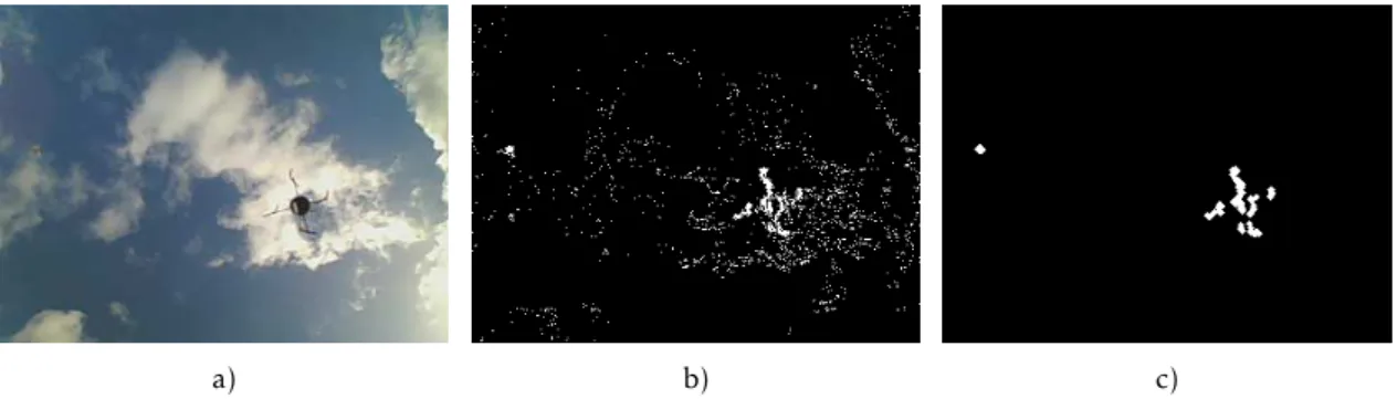
5.2 Data-set representative frames . . . 53
5.3 Object Detection frame classification . . . 54
5.4 Effect of sudden luminosity variations. . . 55
5.5 Effect of bad illumination . . . 56
5.6 Effect of the sun on the UAV detection. . . 57
5.7 Effect of sun glares on the Cloud Mask. . . 57
5.8 Objects Entropy/Uniformity plot . . . 58
5.9 Effect of a UAV and Aeroplane translation movement in the overall optical flow 59 5.10 Zoomed aeroplane and UAV flow patterns. . . 59
5.11 Averaged position delay effect . . . 61
5.12 Error on the computation of the UAVs centre, when its partially outside the camera’s Field of View (FoV) . . . 62
5.13 Creation of an offset between the camera and the landing surface. . . 62
5.14 A general overview of the simulation environment . . . 63
5.15 Simulated helipad’s camera. . . 64
5.16 Simulation camera, with and without offset between helipad and camera . . 64
5.17 Velocity commands example in 3D perspective obtained via simulator . . . . 65
L i s t o f Ta b l e s
5.1 MoG and cloud mask parametrisation . . . 50
5.2 Clustering Parametrisation . . . 50
5.3 Classifier Parametrisation . . . 51
5.4 Tracking Parametrisation . . . 51
5.5 Frame weights user for the computation of the UAV average position . . . 51
5.6 Control Parametrisation . . . 52
5.7 Object Detection Results . . . 54
5.8 Tracker Results . . . 60
G l o s s a r y o f t e r m s a n d A c r o n y m s
AI Artificial Intelligence (AI) is the theory and development of com-puter systems able to perform tasks normally requiring human intel-ligence. Encompasses fields such as visual perception, speech recogni-tion, decision-making, language translation etc.
AR Augmented Reality (AR) is a direct or indirect live view of a physical, real-world environment whose elements are enhanced by computer-generated perceptual information.
Blob Blob is a continuous, generally white pixel zone in a binary mask. Each blob is usually considered an object of interest for further analysis.
BS Background Subtraction (BS) is a technique in Computer Vision used to extract objects of interest in an image or video. Generally there is a static background, in front of which objects move. The algorithm detects those moving objects by computing the difference between the
current frames and a background model previously established.
Camshift Tracking algorithm that uses colour signatures as input. It works by locating the maximum value of density functions, for example, finding the zone in a image where the density of pixels of a given colour are maximized.
G L O S SA RY O F T E R M S A N D AC R O N Y M S
CCL Connected Component Labelling (CCL) is an algorithm based on graph theory used for the detection of regions in binary digital images.
CMOS Complementary Metal-Oxide-Semiconductor(CMOS) is a technology for constructing integrated circuits. It uses complementary and sym-metrical pairs of p-type and n-type metal oxide semiconductor field effect transistors for the creation of logic functions.
CPU Central Processing Unit (CPU) is a electronic circuit that carries out the instructions of a computer program by performing basic arithmetic, logical, control and input/output (I/O) operations. It is generally the component that perform most of the computation in a computer.
CV Computer vision (CV) is the field that develops methods to acquire high-level understanding from digital images or videos.
FoV Field of View (FoV) is the extent of observable world by an given ob-server, a person or camera. It is generally measured in degrees.
GPS Global Positioning System (GPS), is a satellite-based radio navigation system, designed for outdoors. It provides geo-location and time infor-mation to receivers anywhere on Earth.
GPU Graphics Processing Unit (GPU) is a circuit designed to rapidly manip-ulate and alter memory to accelerate the creation of images in a frame buffer intended for output to a display device. It has highly parallel
architecture, making highly adept to perform multiple task at the same time.
IMU Inertial Measurement Unit (IMU) is an electronic device that measures and reports forces, angular rate, and the magnetic field surrounding it. Generally composed by a combination of accelerometers, gyroscopes and magnetometers.
G L O S SA RY O F T E R M S A N D AC R O N Y M S
KDE Kernel Density Estimation (KDE) is a non-parametric method used to estimate the probability density function of a random variable.
KF Kalman Filter (KF) is an algorithm that uses a series of measurements observed over time, containing statistical noise and other inaccuracies, and produces estimates of unknown variables that tend to be more accurate than those based on a single measurement alone.
LIDAR Light Detection And Ranging (LIDAR) is a optic technology for de-tection, that measures reflected light to obtain the distance between objects. Generally is performed by emitting a laser light and measuring the time spent between the emission and the reception of the laser’s reflection.
ML Machine Learning (ML) is the field of computer science that tries gift computer systems with the ability to "learn", i.e., progressively improve performance in a specific task.
MoG Mixture of Gaussian (MoG) is a method that consists on combining mul-tiple Gaussians into a single Probability Density Function, improving the representation of sub-populations present within the general one. In CV it is associated with Background Subtraction methods.
MR-VTOL Multi Rotor-Vertical Take OffLanding (MR-VTOL) are UAVs equipped
with multiple rotors attached to propellers set parallel to the ground. Thus are capable of landing and taking offvertically just like a
heli-copter.
NN Neural Network (NN) is as computational model inspired by animals central nervous system capable progressively learning and recognizing patterns.
G L O S SA RY O F T E R M S A N D AC R O N Y M S
OpenCV Open Computer Vision (OpenCV) is a library of programming func-tions aimed at real-time computer vision. It provides common low-level operations as well as implementations of high-level algorithms.
PDF Probability Density Function (PDF) is a function whose value at any given point in the sample space represents the likelihood of random variable being equal to the value at that point.
PID Proportional Integrative Derivative (PID) is a control loop feedback mechanism used in a wide variety of applications. It computes the error value as the difference between a desired set point and the measured
value and applies a correction based on three variable denominated P,I,D, hence its name.
RANSAC RANdom SAmple Consensus (RANSAC) is an iterative method to esti-mate parameters of a mathematical model from a set of observed data that contains outliers.
RGB Red Green Blue (RGB) is an additive colour model in which red, green and blue light are added together to reproduce a broad array of colours.
ROS Robot Operating System (ROS) is a middleware, i.e. collection of soft-ware frameworks, for the development of robot softsoft-ware. It provides services designed for heterogeneous computer clusters such as hard-ware abstraction, low-level device control, implementation of com-monly used functionalities, message-passing between processes, and package management.
SURF Speeded Up Robust Features (SURF) is a patented local feature detector and descriptor. It can be used for tasks such as object recognition, image registration, classification or 3D reconstruction.
UAV Unmanned Aerial Vehicle (UAV) is a robotic aircraft without a human pilot aboard. It is generally capable of sensory data acquisition and information processing.
G L O S SA RY O F T E R M S A N D AC R O N Y M S
UGV Unmanned Ground Vehicle (UGV) is a vehicle that operates while in contact with the ground without onboard human presence.
USV Unmanned Surface Vehicle (USV) is a robotic element designed to nav-igate over the water’s surface. Generally capable of sensory data acqui-sition and information processing.
L i s t o f S y m b o l s
P
i,s,t Covariance matrix of theithGaussian mixture of pixelsat the timet.
τ Background Subtraction distance threshold.
η Gaussian Probability Density Function.
λ Background Subtraction foreground threshold. Represents the
maxi-mum deviation a pixel can have to belong to the background.
γ Non-negative weight factor between the even and the odd parts of the
Farneback signal.
η(Is,t, µi,s,t,Pi,s,t) Gaussian Probability Density Function of pixelsat the timet.
∆T Time lapse.
∆RGB Difference between RGB channels maximum and minimum value.
αg Gompertz curve maximum value.
γg Gompertz curve scale factor.
βg Gompertz curve offset.
ωi,s,t Weight of theithGaussian mixture.
µi,s,t Mean of value of theith Gaussian mixture of pixelsat the timet.
L I S T O F S Y M B O L S
ρmog MoG secondary learning rate.
ψvc Yaw orientation of the velocity command.
θvc Pitch orientation of the velocity command.
φvc Roll orientation of the velocity command.
∆maxpos Maximum admitted variance in the UAV position between frames.
A Farneback signal matrix.
Akf Transition matrix of Kalman Filter.
B Blue channel of a pixel.
Bg Image background model.
Cl Cloud mask.
Df Frame diagonal (pixels).
Duav UAV’s real dimension (m).
F(x, y) Optical flow at coordinate (x, y) in between two frames.
G Green channel of a pixel.
H(s) Entropy of samples.
Hkf Measurement matrix of Kalman Filter.
Hmog Most reliable Gaussians used for background model computation.
I Pixel intensity/colour value.
I(x, y, t) Pixel intensity at coordinates (x,y) at the timet.
L I S T O F S Y M B O L S
Is,t Intensity of the pixelsat the timet.
K Number of mixtures used in a Mixture of Gaussian.
L(s) Length of the trajectory of samples.
Navg Number of frames used for the computation of the average UAV posi-tion.
Nof Number of frames used for Optical Flow analysis.
P(Is,t) Probability of colourI, in the pixelsat the timet.
Puav UAV’s 3D position.
Qkf Covariance matrix of Kalman Filter.
R Red channel of a pixel.
Sc Cluster set.
T Orientation Tensor.
Tmog Parametrizable threshold measuring the minimum amount of data to be
accounted for the background computation in a Mixture of Gaussians.
V Video Sequence.
Vx Motion flow in thexaxis.
Vy Motion flow in theyaxis.
X X axis of the helipad 3D coordinates frame.
L I S T O F S Y M B O L S
Xs Foreground mask.
Y Y axis of the helipad 3D coordinates frame.
Z z axis of the helipad 3D coordinates frame.
aaz Approach zone curve scale factor.
az(x) UAV’s landing approach zone.
b Vector used for the signal approximation of a neighbourhood of a pixel in the Farneback algorithm.
baz Approach zone curve offset factor.
c Scalar used for the signal approximation of a neighbourhood of a pixel
in the Farneback algorithm.
ck Cluster numberk.
cmax Maximum value of the RGB channels.
cmin Maximum value of the RGB channels.
cth Clustering distance threshold.
cthmin Minimum value ofcth.
cthrat Contribution ratio forcthby the UAV size when compared to the frame
size.
d(s) Minimum radius of samplestrajectory.
daz Ratio between az(x) anddh.
dbs Background Subtraction distance metric.
L I S T O F S Y M B O L S
derror Distance between real position of the in UAV the image and tracker
output in a frame.
dh Distance between UAV and helipad plane parallel to it.
duav UAV’s apparent size in a frame (pixels).
f Camera’s focal length(m).
hbs Background Subtraction history for background model computation.
ith Mixture number in MoG.
km K-Means number of clusters.
kvc θvc normalizing factor.
mvc Velocity command magnitude.
n Frame number.
pavg Weighted average UAV 2D position.
pck(x,y) Central position of clusterk.
pkf UAV 2D position computed by the Kalman Filter.
ps Interval of pixels between samples for Optical Flow analysis.
rck Radius of clusterk.
rbmax Maximum RB ratio for a pixel to belong to the cloud mask.
rbmin Maximum R
B ratio for a pixel to belong to the cloud mask.
L I S T O F S Y M B O L S
s1, ..., st Pixel past values.
sn(x,y) Pixel of framenat position (x,y).
sat Saturation value of a colour.
satmax Maximum saturation value for a pixel to belong to the cloud mask.
t Time instant.
u(s) Uniformity of samples.
vc Velocity command issued to the UAV.
vx UAV’s speed on the x axis in between frames (pixel/miliseconds).
vy UAV’s speed on the y axis in between frames (pixel/miliseconds).
wn Weight of the framenfor the computation of the average UAV position.
x 2D Position on the x axis of an image.
xuav UAV’s 3D position in the x axis.
y 2D Position on the y axis of an image.
yuav UAV’s 3D position in the y axis.
zuav UAV’s 3D position in the z axis.
dx Distance to the image centre in the x axis(pixels).
C
h
a
p
t
e
r
1
I n t r o d u c t i o n
1.1 The applications of UAVs
Just like most technological advancements and innovations in the history of mankind, Unmanned Aerial Vehicle (UAV)s were originally developed for war. UAVs possess the ability to transmit to the battlefield commander, real-time intelligence, surveillance and reconnaissance information from hostile areas. They can also act as communication relays, designate targets for neutralization, or even actively participate in the battlefield by engaging targets themselves. All of this can be achieved without ever putting at risk the lives of a human aircrew [1]. For all these reasons they quickly became an indispensable asset in the hands of military forces all around the globe.
In recent years, UAVs have become a prominent technology not only to military but also in robotics and the general public. Multi-rotor vehicles, in particular, capable of vertical take-offand landing (MR-VTOL), offer high versatility, have relatively low
pro-duction cost, and are easier to teleoperate than their fixed-wing counterparts. Thus they have become an attractive asset in a vast number of scientific and civil applications as well as for recreational purposes. Nowadays UAVs are used in the most diverse areas such as:
Natural Disasters One of the most obvious assets of a UAV is its mobility, being able to get basically anywhere no matter the access conditions. UAVs can be the first to reach zones affected by natural disasters such as hurricanes or tsunamis. Imagery
C H A P T E R 1 . I N T R O D U C T I O N
team was deployed to conduct the post-disaster inspection of bridges, seawalls, and damaged piers, a similar application to the one presented in [4]. In this case, the UAV and USV cooperative work was able to extend or complement the individual capabilities of both. For example, the UAV would acquire imagery that the USV could use to plan its route through the affected zone [5].
Delivery With the increase of e-commerce, giant companies like Amazon and UPS are
faced with the problem of increasing their delivery capabilities. One possible so-lution is the use of UAVs. After the introduction of Amazon’s own UAV delivery service, called Prime Air, some products bought on Amazon’s website can be deliv-ered in just 30 minutes. Competition with other companies in the goods delivery industry, like UPS, increased tremendously due to the introduction of services like these [6]. There are actually studies in ways to use UAVs to extend delivery capa-bilities, with delivery trucks acting as base stations. While the delivery staff do
deliveries, multiple UAVs can be released and make other deliveries in the neigh-bourhood and quickly return, if a problem arises with one of the UAVs, the delivery staffshould be close by and prepared to solve it. In fact, 80% of the packages
de-livered through internet shopping are light enough for a UAV to carry [7], so it is foreseeable that this method and other similar systems for delivery may grow in the future.
Farming and Agriculture Even in Agriculture, Robotics, in particular UAVs, can have
an important role. In [8] a system with a symbiotic relationship between a UAV and a Unmanned Ground Vehicle (UGV), is described. Its goal was the collection of nitrogen levels across a farm for precision agriculture. UAVs are also capable of monitoring and acquiring footage to create panoramas, through geo-referencing and image stitching, that can be used to take decisions about future plantations [9].
Surveillance Surveillance and monitoring is another field that could benefit from UAV technology. In [10] teams of autonomous UAVs are used to monitor complex urban zones, maximizing their coverage through coordination algorithms. This could, for example, be applied in conflict zones, to detect imminent threats. Other possible application of UAVs in surveillance, is in the maintenance of infrastructures. For instance, [11] presents a method for the detection of power lines using Computer Vision (CV) on footage obtained from UAVs. Other applications such as traffic and
crowd monitoring, accident detection, etc, could also be an interesting field to be developed in the future [12].
These are just some examples of possible UAV applications. With the continued development of technology, and the increased processing power of our computers, UAV applications become almost limitless. It may not be too far-fetched to believe that in the future our skies will be filled with UAVs designed for the most various tasks of our everyday life.
1 . 2 . T H E P R O B L E M
1.2 The problem
Generally, independently of its purpose or capabilities, there are two manoeuvres any UAV must be able to perform: taking offand landing. Landing, in particular, is a
espe-cially delicate process since a failed landing can result in damage to the UAV itself, other equipment in the field or even worse, put at risk the safety of people in the surroundings. Landing requires precise control of the UAV and reliable knowledge of the location of both the UAV and the landing zone.
One of the possible ways to perform this manoeuvre is manually through a human operator. This has several disadvantages, the most obvious being human error. The success of the landing rests entirely in the hands of the operator and his skill, which could be proven unreliable or unavailable. Furthermore, having one dedicated person to perform every single landing, wastes manpower that could be spent in other, more productive, endeavours. An alternative is to develop an autonomous system capable of landing on a fixed pad, whose position the UAV can either know beforehand or detect through the processing of sensory information, such as RGB (Red Green Blue) imagery. One more interesting and difficult approach would be to have a mobile platform, a USV
or UGV, acting as a mobile base for the UAV. This last approach requires cooperation between the two robotic systems, which represents an overall increase in complexity. However, a cooperative system like this can vastly expand the capabilities of both robots, improving their performance on the field [4]. The design of such a system requires the use of different technologies like Computer Vision (CV) algorithms, robot communication,
cooperation behaviours, Artificial Intelligence (AI), etc.
C H A P T E R 1 . I N T R O D U C T I O N
avoid making its detection harder or downright impossible.
1.3 Proposed solution
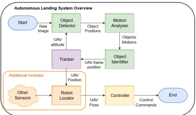
This dissertation proposes a cooperative vision-based landing system for MR-VTOL UAVs, that attempts to solve some of the issues traditional pattern-based systems face. Rather than performing the landing by itself, the UAV receives and relies on information made available by the helipad. The helipad becomes, in essence, a smart element capable of sensory data acquisition and information processing that may, or may not, be coupled to a mobile platform. A camera is put at the centre of the helipad, pointing upwards towards the sky with the objective of detecting the UAV throughout the landing. Therefore a significant part of the computation is moved away from the UAV itself, going to the helipad landing system instead, allowing the UAV to save computational resources and battery life.
The detection method takes advantage of the relatively motionless aspect of the sky, using a Background Subtraction (BS) algorithm, to detect the UAV in the surrounding airspace without the need to rely on a pre-set physical pattern. To distinguish it from other objects, like aeroplanes, the UAV’s chaotic movement patterns, in most part created by the rotation of its propellers, are measured and quantified using an optical flow algo-rithm. After the UAV is correctly detected its position can be extracted and used to relay commands to it, allowing the landing to be performed. A high-level control approach that takes into account the relative positions between, UAV and helipad, is also proposed. The control module establishes an approach zone above the helipad airspace where each deviation from the centre corresponds to a certain velocity command. For each position within the zone, a velocity command with a set orientation and magnitude is issued.
The presented method is generic and modular, designed with the goal of either work-ing as a stand-alone system, performwork-ing the landwork-ing by itself, or bework-ing part of a more complex system. For instance, the system can work together with a traditional approach overcoming or minimizing each other’s shortcomings using multiple cues to perform a more reliable autonomous landing.
1.4 Dissertation Outline
This dissertation is organized as follows:
• Chapter 2reviews the state of the art about UAV automatic landing systems as well as control mechanisms used in this kind of systems. It gives yet a perspective on robot cooperation for the solving of problems like these;
• Chapter 3presents the supporting concepts behind the development of the algo-rithms applied in this work;
1 . 4 . D I S S E R TAT I O N O U T L I N E
• Chapter 4describes the general model proposed, and the reasons for the choices
made during its development;
• Chapter 5goes over the experimental results obtained using the proposed model;
• Chapter 6aggregates the conclusions, the main contributions of this dissertation,
C
h
a
p
t
e
r
2
S t a t e o f t h e A rt
Due to its innate complexity, various different solutions for autonomous landing systems
have been proposed and developed. The need to take into account multiple sensors, having to react to difficulties and external factors in real time, the requirement of precise
controls of the UAV among other issues, make the design of such systems a challenge. This chapter tries to give an overview of the state of the art of vision-based autonomous landing systems, more specifically, the detection method employed as well as the control mechanisms used to manoeuvre the UAV in its descent. At the end of the chapter, a brief synopsis of cooperative systems, and their possible contribution in an autonomous landing system is presented.
2.1 Detection Methods
Computer Vision is a developing field that is generally at the centre of a lot, if not most, of the current auto-landing systems. Its versatility and the wide availability of RGB cameras, when compared to other sensors, makes it especially attractive. Normally vision-based autonomous landing systems can be decomposed into three distinct steps:
1. Analyse the image coming from the UAV or some other asset in the field and extract known features, landmarks or patterns.
2. Estimate the relative position of the extracted features with respect to the camera.
3. After determining all relative positions, it becomes a control problem with the goal of putting the UAV pose on top of the landing pad’s position.
C H A P T E R 2 . S TAT E O F T H E A R T
should be set on a gimbal to minimize trepidation in the captured footage. The UAV starts by approaching the landing pad using an alternative control method that can be for instance, based on GPS (Global Positioning System). When it flies over the landing pad, proceeds to identify the known pattern and then calculate its own relative position to it.
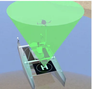
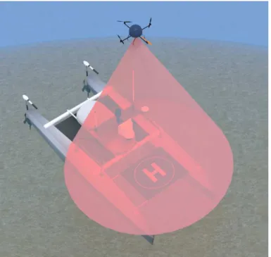
Figure 2.1: Traditional approach for the autonomous landing of MR-VTOL UAVs. The UAV flies to the proximity of the landing zone using, for instance, a GPS-based navigation method. It starts searching for the pre-determined pattern, in this case an “H” inscribed in a circle, with its camera whose FoV is represented by the red cone. After the relative positions are established the landing procedure can start.
The difference between the various approaches mostly lies in the chosen pattern, and
the control method employed. The choice of pattern, in particular, is very important. It has to be distinct enough, to avoid being mistaken with other objects present in the environment, while at the same time simple enough to not overbear the system with great amounts of processing. One of the most common, and simpler, patterns used in this kind of systems is the “H” letter (i.e., initial from Helipad or Heliport), as the one seen in Fig. 2.1. [13] uses a green “H” to perform detection. Knowing the colour of the targeta priori
eases the identification process since a simple histogram analysis of the image, plus a tracking algorithm like Camshift [14], that uses colour signatures as input, allows for good results to be achieved. On top of Camshift a Speeded Up Robust Features (SURF) algorithm is used to locate and identify the features of the “H” pattern. This method only works in simple environments, whereas in more complex environments where other objects in the green spectrum might be present, the method is not robust enough. [15] [16] also use the “H” pattern, but instead of relying on a given colour it is assumed the intensity values of the landing pad are different from that of the neighbouring regions.
The footage obtained from the UAV is converted into a grey scale, using luminance values,
2 . 1 . D E T E C T I O N M E T H O D S
followed by a fixed threshold binarization. The binarized image might contain objects other than the “H” so a Connected Component Labelling (CCL) is used to identify every object, followed by the computation of the invariant moments of every object. From that information, object descriptors are then created and the one whose values most resemble the “H” pattern calibration values is chosen and tracked. Since it doesn’t rely on the pattern having a specific colour, this method is more environment independent, meaning that potentially works on a broader spectrum of surroundings in spite of their colour signatures.
Nonetheless, if the surroundings or multiple objects present in the image, have simi-lar luminance values than the “H”, detection might be compromised. A simisimi-lar example is shown in [17] but instead of using luminance values, a pattern with a negative “H” formed by four white rectangles is used allowing the use of an edge detection algorithm to perform the detection. The edges, the corners of the rectangles, as well as their rel-ative positions are computed and measured to assess if they fit within expected values. Of all letter pattern-based methods this is the most robust since it does not depend on the colours or luminance values of the surroundings. The pattern itself creates visible contrasts, which are used to improve detection. The same idea is applied in [18] where a pattern composed of a black square with smaller white squares in its interior was chosen. The geometric pattern and colour contrasts allow a relatively simple identification pro-cess. Thresholding, followed by segmentation, and finally, corner detection and feature labelling are used. The system is described to be accurate within 5 cm. Yet another similar approach is shown in [19] where an April Tag is used instead for a similar effect.
Another question when choosing the pattern, other than its content, is its size. A size too small might not be able to be identified from high altitudes, requiring the UAV to be at too low altitudes to begin the detection. On the other hand, if the pattern is too big, it may not fit entirely in the camera’s FoV at lower altitudes, or even not fit on the landing pad. This may, or not, be an issue depending on the size of the landing platform and margin of error required. An approach that attempts to solve this problem is presented in [20]. It uses a pattern consisting of several concentric white rings on a black background, where each of the white rings has a unique ratio of its inner to outer border radius. This characteristic makes the identification of a given ring independent of other rings, making it possible to identify the pattern even when it is not completely in view of the UAV. The uniqueness of the pattern, it is said to reduce the number of false positives in both natural and man-made environments.
C H A P T E R 2 . S TAT E O F T H E A R T
a) b) c)
Figure 2.2: Examples of common helipad patterns. Most work by having a presence of high contrasts to facilitate the detection and feature extraction. a) Square shapes together with high contrasts are used to ease corner detection. b) Target-like pattern used in [20], to minimize problems related with pattern size. c) Negative “H” like the one used in [17].
to be run. Motion-based approaches can help overcome the aforementioned problems. Instead of relying on a specific pattern, by using an upwards-facing camera and studying the UAV’s unique motion signature, it becomes possible to create a set of rules that allow for the detection and distinction of the UAV and its relative position to the camera. This method is model-free in the sense that it potentially works for all MR-VTOL UAV’s no matter their configuration (i.e., quad, hexacopters, etc.), colour or shape. Furthermore, the fact the camera is static and facing perpendicularly the ground plane means the process of position estimation is greatly simplified. Most of data processing requirements are also taken away from the UAV itself, allowing, if necessary, more complex algorithms to be run, on more powerful computers on the field, freeing the UAV to focus on other tasks.
2.2 Control
The control of the UAV is a central part of the development of an autonomous landing system. The goal is to put the UAV on top of the landing platform with the most safety possible. For simplicity sake, it is assumed the helipad is parallel to the ground and there are no obstacles present in the airspace above it. The UAV starts from a high altitude, being guided to the helipad by other navigation methods like for example GPS-based ones. After the features, patterns or landmarks are detected it tries to align itself with the centre of the helipad, slowly starting its descent while trying to keep the needed alignment until it has safely landed.
Control can be divided into two areas:
• Low-level:how the motors should be actuated to perform a movement in a certain direction;
• High-level:which movements should be performed in a given situation.
2 . 2 . C O N T R O L
2.2.1 Low-level control
One possible first step is to build a mathematical model of the UAV, as shown in [21], where the Newton-Euler and Euler-Lagrange equations were used to get the multi-rotor flight dynamics, together with quaternions to parametrize the UAV rotations. Quater-nions were used instead of Euler angles as to avoid singularities. A similar approach was used in [22] where the Newton movement laws were used to similar effect. After the
dynamic model of the system is built, either by estimation or by building a mathematical model, it is possible to apply a control loop. A classic solution is the use of a Proportional Integrative Derivative (PID) or any of its possible derivations (PD,PI) [21] [23]. Due to their simplicity and ease of use, PID controllers are one of the most common approaches to perform UAV control, however, despite its simplicity, correct tuning of a PID controller can be a complex matter. In [24] a deadbeat controller is implemented resorting to mul-tiple control loops. The tuning of mulmul-tiple PID may consume a vast amount of time since each PID has three parameters needing to be tuned and generally, there is a need to perform a great number of test flights to achieve the expected performance. Usually, UAV PIDs are tuned to perform under specific conditions, if these conditions change there might be a need to perform some additional tuning, for example, if the payload carried by the UAV changes. Since different weights might affect the flight dynamics of
the UAV in different ways if a given UAV has to change its payload the PID might need
to be tuned all over again. [25] proposes a self tuning PID, based on fuzzy logic to solve this problem. An additional Fuzzy Logic layer is added to the control loop with the goal to make adjustments to the control PID parameters. This way was possible to achieve the expected performance despite payload changes. In [26], fuzzy logic was used as well but as higher lever control system, using the vision sensory data as input, together with a PID for the actual low-level control. Using a Neural Network (NN) is another possi-bility for the control loop, their learning capabilities are ideal for rapid responses and adaptability in uncertain environments. Such a system was developed in [27], where the information coming from the onboard sensors is used to feed the network and control the UAV’s direction and orientation. In [28] a comparison of performance between two controllers one based on a mathematical approach and other based on a neural network system was made, with the NN approach showing to have a similar performance to a purely mathematical approach.
2.2.2 High-level control
C H A P T E R 2 . S TAT E O F T H E A R T
Figure 2.3: Mathematical analysis of a MR-VTOL flight dynamics, adapted from [21]. The UAV has to able to counteract gravity acceleration and so each propeller produces force in opposite direction producing liftfn. Each propeller rotates in the opposite direction(ωn)
of its neighbours to cancel out the UAV’s torque effect. The UAV can be controlled by
individually varying the rotation speed of each propeller.
as needed. [20] uses a two module system: altitude controller, using a sonar sensor for measurements and a PID loop for control; Position and Velocity controller using an optical flow sensor facing the ground as input, both are also controlled via a standard controller (PD and PID respectively). In the landing manoeuvre, the position controller tries to keep the alignment with helipad performing corrections as needed, while the altitude controller slowly performs the descent. [15] and [16] propose a similar architecture but further subdivides the positional controller in lateral velocity controller and heading controller, this way a more granular control of the UAV is achieved.
2.3 Cooperative Systems
Systems composed of multiple robots can be especially interesting to consider. More robots in the field mean more data gathering capabilities, more processing power, etc. Having members with different capabilities, for example, UAVs working together with
USVs or UGVs, extends the capabilities of both allowing them to achieve tasks not pos-sible when working alone. Currently UAVs face two major problems: short flight time due to battery capacity and relatively low computational capacity when compared to full-fledged computers. Both of these problems can be partially overcome with the use of a cooperative system.
Coordination between members of a robotic team, however, can be a real problem. The
2 . 3 . C O O P E R AT I V E S YS T E M S
problem stems from the fact the more data is available the harder is select the relevant information and process it. In centralized systems where all information is available to all members of the system, they can quickly be overloaded with superfluous data, making processing and response times much slower. Furthermore, the scalability of the system may become an impossibility. On the other hand, in a decentralized system where each element of the system has only partial information, the question becomes what information should and should not be shared, and which information should be known by all. Another problem can be what to do when the communication systems fails, how long should old transmitted data be considered etc.
[29] introduces a UAV/UGV three-layer hierarchical cooperative control framework with the intent of being deployed in firefighting. Multiple UAV/UGV teams are deployed in the field, both with distinct objectives, the UAV should travel and drop water to specific points, while the UGV should establish a perimeter and avoid fire proliferation. Hier-archically above them is an airship, responsible for assigning individual tasks to each member in the field while receiving all the data from the UAV/UGV teams.
In [30], a symbiotic relationship between a USV and UAV is described. The USV piggybacks the UAV, saving the UAV’s battery life. On the other hand, the UAV is able to take off, gather sensory information of the surroundings and build a navigation map,
which will later be used by the USV, to create a cost map so it can plan a path. With the help of the UAV, the USV is able to plan much more further ahead than when working alone. The USV helps the UAV’s landing, using its upwards facing camera to detect a pattern, in this case, an Augmented Reality (AR) marker, set on the bottom of the UAV. In turn, the UAV with its own camera learns the appearance of the landing zone during take-off, building a saliency map. This saliency map is then used to help the UAV to
recognize the heliport during landing.
A similar relationship is presented in [8], but instead of a USV a UGV is used. The goal of this system is data collection for precision agriculture, detecting Nitrogen levels across a farm, with the purpose of aiding in fertilizer usage. The main feature of the system just like [30] is the fact the UGV carries the UAV to specific deployment points, decreasing the strain of the UAV battery life, which again, is generally short. Specific points indicated by the UAV should be inspected more closely by the UGV, for this, a path planning algorithm was developed where the UGV takes into account not only his own way-points but also, recovery points for the UAV, minimizing the total time spent in travelling and taking measurements. In summary, the use of cooperative robotic teams can be highly advantageous for the performance of the system as a whole. In the particular case of an autonomous landing system the use of multiple cues coming from different robots can
C
h
a
p
t
e
r
3
S u p p o rt i n g C o n c e p t s
This chapter introduces some key aspects, general concepts and algorithms used as the basis for the development of this dissertation. These are the use of motion patterns for UAV detection and data analysis for its respective identification. Background Subtraction techniques are introduced in section 3.1, whereas Optical Flow (OF) is overviewed in section 3.2. Finally in section 3.3, some phenomena, fast moving and rotating objects provoke when exposed to camera footage are explained.
3.1 Background Subtraction
Background Subtraction is a technique used to detect moving objects from an image, captured by a static camera. Generally speaking BS is performed by subtracting the current frame in relation to a background image, formally called "background model". This background model is an image in the absence of any moving objects, only with its static components. However it should not remain unchanged. In the best BS algorithms the background model must be capable of adapting to varying luminosity conditions, geometry settings, as well as new objects that become part of the background [31].
There are numerous approaches to implement BS algorithms as well as countless variations and improvements. The problem lies in choosing the criteria used to detect the changed pixels and the method to generate the background model. A simple image subtraction wouldn’t suffice since the result would be too sensitive to noise and small
movements of background objects. A BS algorithm generally makes the following as-sumptions, the video sequence,V, has a fixed Background ,Bg, in front of which moving
objects are observed. At any given time,t, a moving object’s colour differs from the colour
C H A P T E R 3 . S U P P O R T I N G C O N C E P T S
Xs=
1 if dbs(Vs, t, Bg)> τ
0 otherwise, (3.1)
whereXsis the motion mask, meaning the pixels belonging to the moving objects;dbsis
the distance at a given pixelsbetween the current frame andBg andτ is a set threshold.
Most BS techniques follow this approach, the difference lying in howBgis modelled
and the metric used to calculate dbs [32]. One of the most common approaches is to
model every background pixel as Probability Density Function (PDF). For example, the Gaussian function can be used together with a log likelihood or Mahalanois distance as the metric fordbs. To reduce the effect of possible slight movements in the background
objects (waves, branches, clouds etc.), multi-modal PDF can be used for the background model representation, for example in [33] each pixel is modelled by a mixture ofK
Gaus-sian distributions. The choice of method depends entirely on the application. Simpler methods like Gaussian average or the median filter offer good reliability while not being
too computationally demanding. Other methods like MoG and Kernel Density Estima-tion (KDE), show better results when compared to simpler methods, being much more resistant to noise. They do, however, have slightly higher memory and processing de-mands and are also harder to implement. All these algorithms have good performance if the camera is static, but it is easy to understand if the camera starts moving they won’t work since the background will be constantly changing. Multiple authors have proposed BS algorithms that work with moving cameras. [34] presents two algorithms capable of distinguishing pixels in consecutive frames into foreground or background by detecting and taking into account independent motion relative to a statistical model of the back-ground appearance. [35] takes into account that all the static parts of the backback-ground lie in the same subspace, to classify the pixels belonging to the foreground and to the background. RANdom SAmple Consensus (RANSAC) algorithm is then run to estimate the background and foreground trajectories. With them, it is possible to create both the background and foreground model.
3.1.1 Mixture of Gaussian
In probability and statistics, a mixture distribution is the merge of multiple mathematical distributions to form a single one. They are particularity useful for the representation of data populations that present multi-modal behaviour i.e., data whose its random variable, has multiple distinct high probability values. Each one of the individual distributions that form the final PDF is called a mixture or a component, and are characterised by their mixture weight (probability) [36].
In CV a mixture of distributions, in particular of Gaussians is associated with a family of BS algorithms commonly called MoG. From all the existent background subtraction techniques MoG is one the most widely used, mostly due to its relative ease of implemen-tation, moderately low computational requirements, high resistance to noise and slight
3 . 1 . BAC KG R O U N D S U B T R AC T I O N
a) b) c)
Figure 3.1: Background Subtraction example. a) The background model represents the image captured by the camera only with its unmoving objects. b) The current frame being analysed, containing one person walking by. c) Since the pixels belonging to the moving person do not fit into the background model, they are marked as white in the foreground mask.
movements, all the while still being capable of achieving good results.
MoG makes the following assumptions: a “foreground model” is segmented by the exception of the background model, meaning every component which does not fit into the background is foreground. This in turn, means the foreground model is not formally modelled either by colour, texture or edges. Model analysis is made per-pixel instead of regions, with each pixel being individually evaluated and decided whether it belongs to the foreground or the background. This decision is made on a frame by frame basis, with-out assumptions abwith-out the object shape, colour or positions. The background model is generated through a cumulative average of the pasthbsframes. The objects are segmented
based on the distancedbsof the individual pixels on the current frame in relation to the
background model [37], with pixel whose values do not fit the background distributions being considered foreground.
The mathematical theory behind MoG is described in [38] and [33], while some im-provements to the algorithm are presented in [39]. MoG uses a mixture of normal (Gaus-sian) distributions to form a multi-modal background Fig.3.3. For every pixel, each distribution in its background mixture corresponds to the probability of observing a particular intensity of colour.
The values of a particular pixel are defined either as scalars, in grey images, or vectors, for colour images. At a given time,t, what is known about a particular pixel,s(x0, y0) is its history:
s1, ..., st=I(x0, y0, i) : 1≤i≤t, (3.2)
The recent history of each pixel, s1, ..., st, is modelled by a mixture ofK Gaussian
C H A P T E R 3 . S U P P O R T I N G C O N C E P T S
P(Is,t) = K
X
i=1
ωi,s,t∗η(Is,t, µi,s,t,Pi,s,t) (3.3)
whereKis the number of distributions used;ηis the Gaussian probability density func-tion;ωi,s,tis an estimate of the weight of theithGaussian in the mixture at the timet;µi,s,t
is the mean value of theithGaussian in the mixture at timetandPi,s,tis the covariance
matrix of theith Gaussian in the mixture at timet; To improve the computational
perfor-mance of the algorithm, in RGB images, it is assumed the red, green, and blue channel values of a given pixel are independent and have the same variance, expressed by:
X
K,t
=σK2∗I (3.4)
After every new frame, ifIs,t is withinλof the standard deviation ofµi,s,t, theith compo-nent is update as follows:
ωi,s,t= (1−αmog)ωi,t−1+αmog, (3.5)
µi,s,t= (1−ρmog)µi,s,t−1+ρmogIi,s,t, (3.6)
σi,s,t2 = (1−ρmog)σi,s,t2 −1+ρmog(Ii,s,t−µi,s,t)2, (3.7)
Whereαmog is a user-defined learning rate andρmog is a secondary learning rate defined asρmog =αmog η(Is,t, µi,s,t,Pi,s,t). If it is not within the standard deviation the update is
instead:
ωi,t= (1−αmog)ωi,t−1, (3.8)
µi,t=µi,t−1, (3.9)
σi,t2 =σi,t2−1, (3.10)
Furthermore, when no component matchesIs,t the component with lowest probability is
replaced by a new one withωi,s,t=Is,t, a largePi,tand smallωi,s,t. After every Gaussian
is updated, the weightsωi,s,tof each one of them are normalized so they add up to 1. The K Gaussian distributions are then ordered based on a fitness value given by: ωi,s,t
σi,s,t,
meaning mixtures with high probability and low variance are deemed to have better quality. Then only the most reliableHmog are chosen as part of the background model, using the criteria:
Hmog =argminh( h
X
i=1
ωi> Tmog) (3.11)
3 . 2 . O P T I CA L F L OW
whereTmog is parametrizable threshold measuring the minimum amount of data that
should be accounted for the background computation. Every pixel at more thanλis
con-sidered to not be part of the background, and so by exclusion, it belongs to the foreground. Furthermore, in some implementations, foreground pixels can be segmented into regions using connected a component labelling algorithm which can be useful for future object analysis and representation.
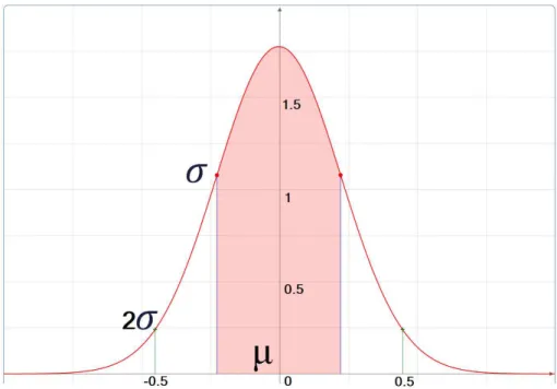
Figure 3.2: Gaussian distribution example. A Gaussian curve can be characterized by two parameters: its mean valueµ, which decides where its centre and maximum point are and its varianceσ which affects the value at the maximum point and smoothness of the
curve. In MoG each Gaussian curve represents the probability of a given pixel having a certain colour. Only the colour intensitiesI, within a certain deviation (for example, the red area) are to be considered part of the background.
3.2 Optical Flow
OF is traditionally defined as the change of structured light in an image, e.g. on the retina or the camera’s sensor, due to the relative motion between them and the scene (see Fig. 3.4). OF methods try to calculate and measure the relative motion, certain regions or points suffer, between two image frames taken at timest andt+∆t. These methods
are called differential since they are based on local Taylor series approximations of the
C H A P T E R 3 . S U P P O R T I N G C O N C E P T S
Figure 3.3: Multi-modal Gaussian example adapted from [40]. In MoG each pixel is mod-elled by a multi-modal Gaussian withK mixtures (Gaussian curves). In this particular
figure, 3 curves (blue lines) were used. The final PDF (red line) is obtained by adding each individual mixture. Its local maximums of correspond to the most likely pixel values.
transformed into a line whose direction in the volume has a direct correspondence to its velocity vector [41].
So in a 2D+t geometric space, in essence 3D, a given Voxel (x, y, t) with intensity I(x, y, t) will move∆x,∆yand∆t, between two image frames. A brightness constraint can
be set by:
I(x, y, t) =I(x+∆x, y+∆y, t+∆t), (3.12)
Supposing the movement between consecutive frames to be small:
I(x+∆x, y+∆y, t+∆t) =I(x, y, t) + ∂I ∂x∆x+
∂I ∂y∆y+
∂I
∂t∆t+H.O.T . (3.13)
where H.O.T means Higher Order Terms.
∂I ∂x∆x+
∂I ∂y∆y+
∂I
∂t∆t= 0 (3.14)
∂I ∂xVx+
∂I ∂yVy+
∂I
∂t = 0 (3.15)
where Vx and Vy are the x and y components of the velocity or flow of I(x, y, t) and ∂I
∂x,∂I∂y and ∂I∂t are the derivatives of the image at (x, y, t). Working eq.3.15 the following is
obtained:
IxVx+IyVy=−It (3.16)
This equation has two unknown variables,Vx andVy, and so it cannot be solved by itself. This is known as the aperture problem of optical flow algorithms [42]. The direction
3 . 2 . O P T I CA L F L OW
vector of the movement of a contour, observed from a small opening, is ambiguous due to the fact the parallel motion component of a line cannot be inferred based on the visual input. This means that a variety of contours of different orientations moving at different
speeds can cause identical responses in a motion sensitive neuron in the visual system, either an eye or a camera sensor, as illustrated in fig.3.5. OF methods introduce additional constraints, that add new equations to the mix allowing eq.3.16 to be solved.
Figure 3.4: Optical Flow example adapted from [42]. Optic flow is perceived by the observer, in this case, an eye retina, as changes in the patterns of light captured by it. The image displays the positions changes of visual features (star and hexagon) on a plane and their respective displacements as perceived by the eye. If the structured light is captured for instance by a camera it is sampled spatially and temporally resulting in an image sequence. The three frames show the movement of a head. The optic flow is depicted as the correspondence of contour pixels between frames (1 and 2, 2 and 3). Optical Flows techniques search for ways to compute this correspondence for each pixel in the image.
3.2.1 Farneback Algorithm
C H A P T E R 3 . S U P P O R T I N G C O N C E P T S
Figure 3.5: Aperture problem example retrieved from [43]. The images represent a moving sequence. It is impossible to access the direction of the movement by observing only a portion of the object.
development of this method can be done by looking at [41], and additional improvements in [44] and [45].
The algorithm uses the concept of orientation tensors to represent local orientation. Movement in an image sequence creates structures that acquire certain orientations in the 3D space. Like mentioned before a translating point is transformed into a line whose direction in the 3D space directly corresponds to its velocity. The use of tensors allows for a more powerful and easier representation of such orientations. The tensor takes the form of a 3 by 3 symmetric positive semi-definite matrixT and the quadratic form ˆuTTuˆ, which is interpreted as a measure of how much the signal varies locally in the direction given by ˆu.
The orientation tensors are computed by polynomial expansion. Since an image can be seen as a two-dimensional signal, the neighbourhood of each pixel signal can be projected into a second-degree polynomial, following the model:
f(x) =xT∗A∗x+bTx+c (3.17)
whereAis a symmetric matrix,bis vector andca scalar. These parameters are computed
by a weighted least squares approximation of the signal values in the neighbourhood, where the weighting function is a Gaussian.
From the model parameters, an orientation tensor is constructed by:
T =AAT+γbbT (3.18)
whereγ is a non-negative weight factor between the even and the odd parts of the signal.
The 2D velocity vector (vxvy)T, can be extended to a 3D spatio-temporal directional
vector v: v= vx vy 1 (3.19) ˆ
v= v
||v|| (3.20)
3 . 3 . I M AG E CA P T U R E E F F E C T S
Instead of estimating the velocity from the tensors for each point it is assumed that the velocity field over a region can be parametrized according to some motion model:
vx(x, y) =ax+by+c, (3.21)
vy(x, y) =dx+ey+f , (3.22)
wherex andy are images coordinates. This can be yet converted into a spatiotemporal
vector as:
v=Sp, (3.23)
S=
x y 1 0 0 0 0 x 0 0 x y 1 0
0 0 0 0 0 0 1
(3.24) p=
a b c d e f 1T (3.25)
by further adding mathematical constraints and cost functionspparameters can be
calculated, and thereforevx andvy [41].
3.3 Image capture e
ff
ects
When fast rotating objects are exposed to camera sensors, certain visual phenomenona can happen. Cameras do not record footage continuously, but rather discretely by capturing series of images in quick succession, at specific intervals. Since cameras can only capture a subset of the positions of a given movement, the motion of rotation cannot be fully represented. Therefore if the rotation speed of an object is significantly faster than the capture frame rate, the object will appear to perform jumps in its rotation. Furthermore depending on the sensor type present in the camera two distinct capture modes, Charged Coupled Device (CCD) or Complementary Metal-Oxide-Semiconductor (CMOS), might cause other phenomena to happen:
• Rolling Shutter;
• Global Shutter.
A rolling shutter effect happens when cameras with a rolling shutter are used, as in
most cameras with a CMOS sensor. When in a rolling shutter mode, pictures or frames from a video sequence are captured, by scanning across the scene in a short amount of time, either vertically or horizontally. This results in the adjacent rows or columns of the array of sensor cells being exposed at slightly different times, essentially creating waves
C H A P T E R 3 . S U P P O R T I N G C O N C E P T S
a) Rolling Shutter b) Global Shutter
Figure 3.6: Rolling and Global shutter effects example retrieved from [46]. a) Using the
rolling shutter the deformation on the fan’s pads is visible producing a dragging-like effect. b) In the global shutter, the fan is like frozen in time without presenting any
deformation.
slight offset in time when compared to its neighbours. Despite this during playback, the
entire image of the scene is displayed at once, as if it represents a single instant in time. This produces predictable distortions of fast-moving objects or rapid flashes of light seen in Fig. 3.6a).
On the other hand, global shutter is a mode where every pixel of the image is cap-tured simultaneously. Since there are no delays between neighbour rows, global shutter achieves an effect of a frozen image, reducing distortions as shown in Fig. 3.6b).
Yet another effect that can happen, is called the “wagon-wheel” effect. When the
frequency of a wheel or a propeller’s spin matches the frame rate of the camera recording it, each of the wheel’s spokes or propeller blades completes a full revolution, ending up in the same position every time the camera captures a frame. Giving the sense they are motionless. However if the rotation speed changes and gets slower, the wheel or propellers will start to be a few degrees shy of their positions when compared to the last frame, and so they will seem to slowly rotate in the opposite direction.
Rotating propellers are one of the possible origin of these effects, they generate
irreg-ular and chaotic patterns when exposed to cameras, that can be useful to perform their identification in camera footage. For example, they might be used to identify a motion signature that might correspond to an UAV.
![Figure 3.3: Multi-modal Gaussian example adapted from [40]. In MoG each pixel is mod- mod-elled by a multi-modal Gaussian with K mixtures (Gaussian curves)](https://thumb-eu.123doks.com/thumbv2/123dok_br/16571921.738054/48.892.243.639.165.420/figure-multi-gaussian-example-adapted-gaussian-mixtures-gaussian.webp)
![Figure 3.4: Optical Flow example adapted from [42]. Optic flow is perceived by the observer, in this case, an eye retina, as changes in the patterns of light captured by it](https://thumb-eu.123doks.com/thumbv2/123dok_br/16571921.738054/49.892.189.705.312.807/figure-optical-example-adapted-perceived-observer-patterns-captured.webp)
![Figure 3.6: Rolling and Global shutter e ff ects example retrieved from [46]. a) Using the rolling shutter the deformation on the fan’s pads is visible producing a dragging-like e ff ect](https://thumb-eu.123doks.com/thumbv2/123dok_br/16571921.738054/52.892.134.761.156.452/figure-rolling-global-shutter-retrieved-deformation-producing-dragging.webp)