Diana Sofia Gusmão Coito Madeira

(1)

Effects of ocean warming throughout the life

cycle of

Sparus aurata

: a physiological and

proteomic approach

Dissertação para obtenção do Grau de Doutor em Química Sustentável

Orientador: Mário Sousa Diniz, Professor Auxiliar,

Faculdade de Ciências e Tecnologia

Universidade Nova de Lisboa

Co-orientadores: Catarina Vinagre, Investigadora Auxiliar,

Faculdade de Ciências

Universidade de Lisboa

José Luís Capelo, Professor Auxiliar,

Faculdade de Ciências e Tecnologia

Universidade Nova de Lisboa

Júri:

Presidente: Doutora Ana Isabel Nobre Martins Aguiar de Oliveira Ricardo, Professora Catedrática da Faculdade de Ciências e Tecnologia da Universidade Nova de Lisboa Arguentes: Doutor Henrique Manuel Roque Nogueira Cabral, Professor

Catedrático da Faculdade de Ciências da Universidade de Lisboa Doutora Maria Teresa Garrett Silveirinha Sottomayor Neuparth, Investigadora de Pós-Doutoramento do Centro Interdisciplinar de Investigação Marinha e

Ambiental (CIIMAR) da Universidade do Porto Vogais: Doutora Maria Helena Ferrão Ribeiro da Costa, Professora

Associada com Agregação da Faculdade de Ciências e Tecnologia da Universidade Nova de Lisboa Doutora Maria Gabriela Machado de Almeida, Professora Associada do Instituto Superior de Ciências da Saúde Egas Moniz

(2)

(3)

Diana Sofia Gusmão Coito Madeira

Mestre em Ecologia Marinha

Effects of ocean warming throughout the life-cycle of

Sparus aurata

: a physiological and proteomic approach

Dissertação para obtenção do Grau de Doutor em Química Sustentável

This thesis was supported by a Fundação para a Ciência e Tecnologia, fellowship, reference number SFRH/BD/80613/2011

(4)

(5)

Effects of ocean warming throughout the life-cycle of Sparus aurata: a physiological and proteomic approach

(6)

(7)

A

CKNOWLEDGEMENTS

I wish to express my gratitude to all people that guided, helped and contributed to this work, in particular to:

Professor Dr. Mário Diniz for the supervision of this work, for the invaluable guidance and friendship, expertise and advice, for trusting me and letting me explore new ideas, for understanding and encouraging me throughout the ups and downs of this work.

Dr. Catarina Vinagre for the supervision of this work, for the encouragement, joyfulness and friendship, for the splendid tips and advice, for providing moral support in the toughest moments, for inviting me to participate in awesome field trips to renew my motivation.

Professor Dr. Luís Capelo for the supervision of this work, advice and thoughtful exchange of ideas throughout this thesis.

Dr. Pedro Costa for all the guidance and comradeship, precious advice given during all crucial stages of this work, for teaching me in detail all about histopathological analysis, for understanding my ups and downs and for always putting forward interesting discussions.

Dr. Rui Vitorino for all the guidance, expertise, and work and for the tremendously helpful tips, which were all crucial to achieve several of the research aims.

MARESA, for providing Sparus aurata and fish food supplies free of charge or at lowered price.

My wonderful and cherished colleagues from Faculdade de Ciências e Tecnologia da Universidade Nova de Lisboa, namely Eduardo Araújo, Marta Martins, Susana Jorge, Ana Patrícia, Susana Ferreira Silva, Cristina Nuñez Gonzalez, Ana Luísa Maulvault and Ana Filipa Silva for the understanding, friendship, cheering and joyful moments we shared; for the priceless support you provided throughout the darkest and the brightest times!

My awesome colleagues from the ECCOWEBS group (Faculdade de Ciências da Universidade de Lisboa), namely Vanessa Mendonça, Marta Dias, Rui Cereja and Pedro Fernandes for the marvelous friendship, fun times, field trips, laughter and true companionship and mutual support.

My former colleagues, which encouraged me and still managed to help me at a distance. I wish to express my thanks specifically to Miguel Leal, Marco Galésio, Ricardo Carreira, Gonçalo Vale, Íris Batalha, Miguel Larguinho, Carla Martins and Cátia Gonçalves for their warm support, knowledge and friendship.

My friends Rita, Catarina, Vanessa Leal, Teixeira, Araújo, Abreu and Jota for all the support and friendship, which were essential to help me get through these 4 years of hard work.

(8)

(9)

R

ESUMO

As alterações climáticas são um problema ambiental com efeitos persistentes nos ecossistemas marinhos, afectando os serviços ambientais fornecidos por estes à sociedade, provocando alterações na biodiversidade, abundância e distribuição das espécies, interacções biológicas, fenologia e fisiologia dos organismos. No entanto, a vulnerabilidade dos recursos pesqueiros ao aquecimento do oceano é pouco clara devido à falta de abordagens integradas que avaliem processos fisiológicos e moleculares, e que elucidem a forma como estes se alteram ao longo do ciclo de vida dos organismos. Esta tese tem como objectivo estudar a vulnerabilidade duma espécie de peixe comercial, a dourada (Sparus aurata), ao aquecimento

do oceano ao longo do seu ciclo de vida, ao nível molecular, celular e do indivíduo. Os bioensaios realizados revelaram que a fase larvar é especialmente sensível a um aumento agudo ou crónico de temperatura (>22ºC). O CTmax (máximo térmico crítico) das larvas foi de 30ºC e estas mostraram uma capacidade reduzida de induzir a resposta celular ao stress

(levando à desnaturação de proteínas), assim como de alterar o seu metabolismo energético de forma a lidar com o aumento de temperatura. Como tal, foram registadas taxas de mortalidade elevadas, associadas a lesões nos tecidos (ex: músculo e rins). A fase juvenil foi a mais resistente ao aquecimento da água, apresentando um CTmax de 35.5ºC, embora temperaturas iguais ou superiores a 28ºC no ensaio de stress agudo tenham provocado lesões

severas nos tecidos, possivelmente associadas a uma desnaturação proteica e a stress oxidativo. A exposição a stress térmico crónico levou à indução da resposta celular ao stress

(CSR) associada a um aumento do potencial glicolítico (os órgãos vitais foram especialmente reativos), no entanto, após 21 dias de exposição foram detectados sinais de inflamação nos tecidos analisados e observou-se um aumento significativo da mortalidade. A fase adulta mostrou-se menos resistente do que a juvenil uma vez que os órgãos vitais não apresentaram uma grande capacidade de resposta, e foram os que sofreram maiores alterações nos tecidos (ex: danos nos lípidos e proteínas, inflamação, atrofia), causando uma mortalidade elevada. Isto sugere que os adultos não possuem muita plasticidade para lidar com o aumento da temperatura da água. Por conseguinte, o esforço e mecanismos induzidos como defesa ao

stress térmico são diferencialmente alocados consoante o órgão e o estadio de

desenvolvimento. Deste modo, conclui-se que a fase larvar é o estadio de desenvolvimento chave, que irá determinar o fecho do ciclo de vida da dourada num cenário de aquecimento global.

Palavras-chave: temperatura, alterações climáticas, peixes, fisiologia, proteómica, ciclo de

(10)

(11)

A

BSTRACT

Climate change is a major environmental problem, known to cause pervasive effects on marine ecosystems, impacting goods and services provided to society. It alters biodiversity patterns, abundance and distribution of species, biological interactions, phenology, and organisms’ physiology. However, the vulnerability of fish stocks towards ocean warming is still far from clear due to the lack of integrative approaches that address physiological and molecular compensation mechanisms throughout all the stages of the life-cycle. This thesis aimed at uncovering the vulnerability of a highly commercial sea bream Sparus aurata to ocean warming

throughout the various stages of its life cycle, considering organism-, cellular- and molecular-level approaches. The first two assays revealed that larvae are very sensitive to both acute and chronic thermal stress (>22ºC), showing a CTmax (Critical Thermal Maximum) of 30ºC and a reduced capacity to employ the cellular stress response (leading to protein denaturation) and perform the energetic adjustments that would have been necessary to sustain a temperature increase. This probably led to the observed tissue injury (in muscle and kidneys) and elevated mortality rates. Juveniles were the most resistant and plastic to warming with a CTmax of 35.5ºC although temperatures of ≥ 28ºC in the acute assay induced significant tissue damage related to protein denaturation and oxidative stress. Exposure to chronic warming elicited the cellular stress response coupled with an enhanced glycolytic potential (vital organs were highly responsive). However, after 21 days fish showed signs of inflammation and mortality was significantly increased. Adult fish were less resistant than juveniles because vital organs were less responsive and showed the highest tissue injury level (damage to lipids and proteins, inflammation, atrophy) leading to elevated mortality. This suggests a response to damage rather than a plastic response. Thus, the effort and mechanisms of protection against thermal challenge are differentially allocated by distinct organs, depending on developmental stage. Moreover, the larval phase is the key developmental stage that will determine life cycle closure of S. aurata under the projected ocean warming scenarios.

(12)

(13)

L

IST OF SYMBOLS AND ABBREVIATIONS

A

AAA ATPases, ATPases Associated with diverse cellular Activities Abs, absorbance

ac, acinar cells ACN, acetonitrile

ACT2, Actin, muscle-type 2 ACTM, actin muscle

ADP, adenosine diphosphate Ambic, ammonium bicarbonate AMP, adenosine monophosphate ANOVA, analysis of variance Anti-DNP, anti-dinitrophenol AOX, anti-oxidant

Arg, arginine

ARPC2, actin-related protein 2/3 complex subunit 2 at, adipose tissue

ATP, adenosine triphosphate

B

b, brain

BSA, bovine serum albumin bv, blood vessels

C

CAH1, carbonic anhydrase 1 CaM, calmodulin

CANFA, Canis familiaris

CAT, catalase

CDNB, chloro-2,4-dinitrobenzene CHAAC, Chaenocephalus aceratus

CHAPS, 3-[(3-cholamidopropyl)dimethylammonio]-1-propanesulfonate CHIHA, Chionodraco hamatus

CI, confidence interval CO2, carbon dioxide

CRIGR, Cricetulus griséus

CSR, cellular stress response CTmax, Critical Thermal Maximum CYP1A, cytochrome P450 1A CYPCA, Cyprinus carpio

D

Da, Dalton

DANRE, Danio rerio

DGAV, Direcção Geral de Alimentação e Veterinária DHE3, Glutamate dehydrogenase, mitochondrial DNA, deoxyribonucleic acid

DNPH, 2,4-dinitrophenylhydrazine DOC, Na-deoxycholate

(14)

E

E1, ubiquitin-activating enzyme E2, ubiquitin-conjugating enzyme E3, ubiquitin-ligase

EC, Enzyme Nomenclature

EDTA, ethylenediaminetetraacetic acid EGR1, early growth response protein 1 ELISA, Enzyme-Linked Immunosorbent Assay ENOA, alpha-enolase

EPON 821, epoxy resin 821 Eq, equation

ER, endoplasmic reticulum er, erythrocyte

ERSST v4, Extended Reconstructed Sea Surface Temperature version 4 EST, Expressed Sequence Tag

ey, eye

F

f, filament

FAO, Food and Agriculture Organization of the United Nations fc, fascicles

FELASA, Federation of European Laboratory Animal Science Associations FishStat, fishery statistical time series

fv, fat vacuolation

G

G, gills

G3P, glyceraldehyde-3-phosphate dehydrogenase G6PI, glucose-6-phosphate isomerase

gc, goblet cell

GDIB, Rab GDP dissociation inhibitor beta GDP, guanosine diphosphate

GISS, Goddard Institute for Space Studies Glu, glutamate

GO, gene ontology

GPx, glutathione peroxidase GST, glutathione-S-transferase GTP, guanosine triphosphate

H

H&E, Haematoxylin and eosin histological stain ha, hepatic arterioles

HCl, hydrochloric acid

HEBP1, Heme-binding protein 1 hp, hepatocytes

HRP, horseradish peroxidase

HS90A or HSP90AA1, Heat shock protein HSP 90-alpha Hsc70, heat shock cognate 70 kDa

(15)

Hsp70, heat shock protein 70 kDa HSP71, Heat shock 70 kDa protein 1 HSP7C, Heat shock cognate 71 kDa protein Hsp90, heat shock protein 90 kDa

HSPA8, heat shock 70kDa protein 8 Hsps, heat shock proteins

I

I, intestine

IAA, iodoacetamide

IBR, Integrated Biomarker Response ICTPU, Ictalurus punctatus

IEF, isoelectric focusing

IF4A2, eukaryotic initiation factor 4A-II IgG, immunoglobulin G

IPCC, Intergovernmental Panel on Climate Change IPG, immobilized pH gradient

IQCA1, IQ motif containing with AAA domain 1 IQCAL, IQ and AAA domain-containing protein 1-like

IUCN, International Union for Conservation of Nature and Natural Resources

K

K2C8, keratin, type II cytoskeletal 8 KAD1, adenylate kinase isoenzyme 1 KCl, potassium chloride

KCRM, creatine kinase M-type KCRT, creatine kinase testis isozyme kDa, kilodalton

KH2PO4, monopotassium phosphate

KIF2A, kinesin heavy chain member 2A KIF5C, kinesin heavy chain isoform KRT, keratin 8

KRT19, keratin 19

L

L, liver L:D, light:dark Leu, leucine LIZAU, Liza aurata

LIZRA, Liza ramada

lm, lamella lp, lamina propria LPO, lipid peroxidation

M

m, muscle

MACFA, Macaca fascicularis

MALDI, matrix-assisted laser desorption/ionization MAPK, mitogen-activated protein kinase

MARE, Marine and Environmental Sciences Centre MDA, malondialdehyde bis(dimethylacetal)

MELGA, Meleagris gallopavo

(16)

MOLOC, Molgula oculata

mRNA, messenger ribonucleic acid MS, mass spectrometry

MS/MS, tandem mass spectrometry mv, microvilli

MW, molecular weight

N

Na2HPO4, disodium phosphate

NaCl, sodium chloride

NAD, nicotinamide adenine dinucleotide NaOH, sodium hydroxide

NASA, National Aeronautics and Space Administration NBT, nitroblue tetrazolium

NCBI, National Center for Biotechnology Information NEC1, Neuroendocrine convertase 1

NOAA, National Oceanic and Atmospheric Administration of USA NPF, nucleation-promoting factor

NSIDC, National Snow and Ice Data Center Nt, notochord

O

OCLTT, oxygen and capacity limited thermal tolerance Ol, olfactory lobe

ONCMY, Oncorhynchus mykiss

ONCTS, Oncorhynchus tshawytscha

ORYLA, Oryzias latipes

P

p, p-value

PAK, p21 protein activated kinase

PARK2, parkin RBR E3 ubiquitin protein ligase PAS, Periodic Acid-Shiff’s

PBS, phosphate-buffered saline PC, protein carbonylation

PCA, Principal Component Analysis Phe, phelylalanine

PI, isoelectric point PKC, protein kinase C Poly(A), polyadenylation PONAB, Pongo abelii

POTEF, POTE ankyrin domain family member F ppm, parts per million

pr, pancreatic tissue PRIGL, Prionace glauca

PSB3 or PSMB3, proteasome subunit beta type-3 PTM, post-translational modification

PYGB, Glycogen phosphorylase brain form

R

(17)

RGL2, ral guanine nucleotide dissociation stimulator-like 2 RNA, ribonucleic acid

ROS, Reactive Oxygen Species

S

SAM9L, Sterile alpha motif domain-containing protein 9-like sc, spinal chord

SD, standard deviation

SDS, sodium dodecyl sulphate

SIAM, Scenarios, Impacts and Adaptation Measures (Climate Change in Portugal) sk, skeletal muscle

Sm, striated myocytes SOD, superoxide dismutase SOMA, somatotropin

SRES, Special Report on Emission Scenarios SST, sea surface temperature

STYPL, Styela plicata

T

TCA, trichloroacetic acid Tub, total ubiquitin

Tcritical, critical temperature

TBARS, thiobarbituric acid reactive substances Tl, telencephalon

TPIS, Triosephosphate isomerase fragments TPISB, Triosephosphate isomerase B TFA, trifluoroacetic acid

TOF, time-of-flight

TUBA4A, tubulin alpha 4a TPM1, tropomyosin 1 Tyr, tyrosine

Tend-point, temperature at which the end-point is reached

T, tegument

TNF, tumor necrosis factor

TMB, 3, 3', 5, 5' – Tetramethylbenzidine T7, 7 days of exposure

T14, 14 days of exposure T21, 21 days of exposure T28, 28 days of exposure

U

UV, ultraviolet radiation

V

vc, vacuolation

X

XENLA, Xenopus laevis

XENTR, Xenopus tropicalis

XOD, xanthine oxidase

W

(18)

Other

2D, two-dimensional 5'-UTR, leader sequence

, up-regulation

(19)

S

UBJECT INDEX

ACKNOWLEDGEMENTS ... vii

RESUMO ... ix

ABSTRACT ... xi

LIST OF SYMBOLS AND ABBREVIATIONS ... xiii

SUBJECT INDEX ... xix

FIGURE INDEX ... xxv

TABLE INDEX ... xxxv

CHAPTER 1. GENERAL INTRODUCTION ... 1

1. Climate change: global and regional trends ... 3

2. Marine organisms under climate warming scenarios: impacts of rising temperature and the study of thermal tolerance mechanisms ... 7

3. Model organism: Sparus aurata ... 16

4. Relevance to the scientific community and society ... 23

5. Aims, scopes and thesis layout ... 24

Acknowledgements ... 29

References ... 29

CHAPTER 2. WHEN WARMING HITS HARDER: SURVIVAL, CELLULAR STRESS AND THERMAL LIMITS OF SPARUS AURATA LARVAE UNDER GLOBAL CHANGE ... 41

Abstract ... 43

Graphical abstract ... 44

1. Introduction ... 44

2. Materials & Methods ... 47

2.1 Ethical statement ... 47

2.2 Larvae collection and acclimation ... 47

2.3 Experimental setup ... 48

2.4 Protein extraction... 49

2.5 Hsp70 and total ubiquitin (Tub) quantification ... 49

2.6 Antioxidant enzymes... 50

2.7 Lipid peroxidation (LPO) ... 51

2.8 Protein carbonylation (PC) ... 51

2.9 Statistical analysis ... 52

2.10 Histological analysis ... 52

3. Results ... 54

3.1 Critical Thermal Maximum ... 54

3.2 Biomarkers and percent mortality ... 54

(20)

6. References ... 61

CHAPTER 3. OCEAN WARMING ALTERS CELLULAR METABOLISM AND INDUCES MORTALITY IN FISH EARLY LIFE STAGES: A PROTEOMIC APPROACH... 67

Abstract ... 69

2. Methods ... 72

2.2 Assessment of S. aurata thermal environments ... 72

2.3 Housing and husbandry of larvae ... 73

2.4 Experimental assays... 74

2.5 Statistical analysis on survival ... 76

2.7 Proteomic analysis ... 76

2.7.1 Sample preparation... 76

2.7.2 Two Dimensional Gel electrophoresis (2-DE) ... 77

2.7.3 Gel image analysis... 77

2.7.4 Protein digestion ... 77

2.7.5 Mass spectrometry... 78

2.7.6 Database Search ... 78

2.7.7 Expression analysis ... 79

2.7.8 Categorization of identified proteins into functional classes ... 79

3. Results ... 81

3.1 Temperature data ... 81

3.2 Survival curves ... 81

3.3 Proteomic analysis ... 82

4. Discussion... 88

4.1 Chaperoning and protein degradation ... 89

4.2 Cytoskeleton dynamics ... 90

4.3 Intracellular transport ... 91

4.4 Cell-cycle regulation and transcription regulation ... 91

4.5 Growth metabolism ... 91

4.6 Porphyrin metabolism ... 92

5. Conclusions ... 92

6. Acknowledgments ... 94

7. Data Accessibility ... 95

(21)

CHAPTER 4. HISTOPATHOLOGICAL ALTERATIONS, PHYSIOLOGICAL LIMITS AND MOLECULAR CHANGES OF JUVENILE SPARUS AURATA IN RESPONSE TO THERMAL

STRESS ... 103

Abstract ... 105

2. Materials and methods ... 108

2.2 Thermal tolerance method ... 108

2.4 Hsp70 quantification ... 110

2.5 Ubiquitin and ubiquitinated/poly-ubiquitinated protein quantification... 111

2.6 Histological analysis ... 111

3. Results ... 114

3.1 CTmax and Hsp70 ... 114

3.2 Total ubiquitin ... 114

3.3 Correlation between Hsp70 and total ubiquitin ... 116

3.4 Histological observations ... 116

4. Discussion... 121

5. Conclusions ... 125

6. Acknowledgements ... 126

7. References ... 126

CHAPTER 5. ARE FISH IN HOT WATER? EFFECTS OF WARMING ON OXIDATIVE STRESS METABOLISM IN THE COMMERCIAL SPECIES SPARUS AURATA... 131

Abstract ... 133

2. Materials and methods ... 136

2.1 Ethical statements ... 136

2.2 Thermal ramp trial ... 136

2.4 Enzymatic assays ... 138

2.4.1 Catalase ... 138

2.4.2 Glutathione S-transferase ... 138

2.4.3 Superoxide dismutase... 138

2.4.4 Cytochrome P450 1A ... 138

2.5 Oxidative damage products - lipid peroxidation ... 139

(22)

3.3 SOD activity ... 141 3.4 CYP450 1A quantification ... 144 3.5 Lipid peroxidation (LPO) ... 144 3.6 Factor analysis ... 145 4. Discussion... 147 5. Conclusions ... 149 6. Acknowledgements ... 150 7. References ... 150

CHAPTER 6. MOLECULAR PLASTICITY UNDER OCEAN WARMING: INTEGRATING PROTEOME CHANGES WITH ORGANISM-LEVEL INDICATORS UNVEILS THERMAL TOLERANCE OF FISH ... 155

(23)

5. Conclusion ... 182 6. Acknowledgments ... 185 7. Data accessibility... 185 8. References ... 185

CHAPTER 7. LIFE CYCLE CLOSURE OF DEMERSAL FISH IS HAMPERED BY FUTURE WARMING ... 191

Abstract ... 191 1. Introduction ... 194 2. Methods ... 195 2.1 Ethical statement ... 195 2.2 Assessment of Sparus aurata’s thermal environments ... 195

2.3 Housing and husbandry of fish ... 196 2.4 Experimental setup ... 198 2.5 Temperature effects on S. aurata throughout its life cycle ... 198

2.5.1 Mortality and condition index ... 198 2.6 Biomarkers ... 198 2.6.1 Sample treatment ... 199 2.6.2 Biochemical analyses ... 199 2.7 Histopathological procedures ... 199 2.8 Statistical analysis ... 200 2.8.1 Mortality and condition index ... 200 2.8.2 Biomarkers ... 200 3. Results ... 202 3.1 Assessment of Sparus aurata’s thermal environments ... 202

3.2 Temperature effects on S. aurata throughout its life cycle ... 204

3.2.1 Mortality and condition index ... 204 3.3 Biomarkers ... 205 3.3.1 Analysis of variance ... 205 3.3.2 Discriminant and principal components analyses... 208 3.3.3 Integrated Biomarker Response (IBR) ... 209 3.4 Histopathology ... 212 4. Discussion... 214 5. Conclusions ... 217 6. Acknowledgements ... 218 7. References ... 219

CHAPTER 8. CONCLUDING REMARKS AND FUTURE PERSPECTIVES ... 227 ANNEXES ... 233

(24)

(25)

F

IGURE INDEX

Figure 1.1 Global temperature anomalies a) Temperature anomaly for the period of 1980-2014

when compared to the reference period of 1951-1980. The analysis was carried out

in Goddard Institute for Space Studies website (NASA,

http://data.giss.nasa.gov/gistemp/maps/) following the parameters: data sources land (GISS analysis) and ocean (ERSST_v4); mean period annual; time interval 1980-2014; base period 1951-1980; smoothing radius 1200 km; projection type Robinson. Notes: Gray areas are missing data; ocean data are not used over land nor within 100km of a reporting land station; b) and c) Global ocean and land

(respectively) temperature anomalies by year, starting at 1880 until 2014. The right Y axis gives temperature anomaly in degrees Fahrenheit while the right axis is in degrees Celsius (an anomaly of 1ºF is equivalent to an anomaly of 0.556ºC). Source: graphs were obtained using data and tools available in NOAA (National Oceanic and Atmospheric Administration of USA, Department of Commerce,

http://www.ncdc.noaa.gov/sotc/global/201509, accessed

16-11-2015)…...3

Figure 1.2 Trend of sea level change.a) Global mean sea level change compared to the mean

of the baseline period 1980-1999. The gray area shows uncertainty due to the lack of data before 1870. The instrumental record provided in red is based on tidal gauges (mean and variations) and the green line is based on satellite data on altimetry. The blue area represents projections for the future considering scenario SRES A1B. Source: IPCC 2007, with permission. b) Inset of the period

1993-present considering global sea level change based on satellite data. Source: NASA Goddard Space Flight Center (http://climate.nasa.gov/vital-signs/sea-level/, accessed 16-11-2015), with permission. c) Trend of sea level change between

1993-2008 based on satellite data (sea surface height data from the Topex/Poseidon and Jason-1 satellites). Trends of sea level change vary across regions. Source: NASA Jet Propulsion Laboratory, California Institute of Technology (http://photojournal.jpl.nasa.gov/catalog/PIA11002, accessed 20-11-2015), with permission………...5

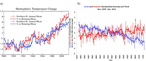
Figure 1.3 Differences in warming trends and ice extent between the Northern and Southern hemispheres. a) Annual and five-year running mean temperature change for

northern and southern hemispheres considering the baseline period from 1951 to

1980. Source: NASA, Goddard Institute for Space Studies

(http://data.giss.nasa.gov/gistemp/graphs_v3/, accessed 16-11-2015), with permission; b) Arctic and Antarctic sea ice extent anomalies and trends concerning the period from 1979 to 2012. Thick lines: twelve-year running means; thin lines: monthly anomalies. Source: National Snow and Ice Data Center (authors: Stroeve J,

Meier W), University of Colorado, Boulder, USA

(https://nsidc.org/cryosphere/sotc/sea_ice.html, accessed 16-11-2015), with

permission………...6

Figure 1.4 Predicted shifts in extreme events. Shifts in extreme events due to changes in

temperature distribution can occur in three ways a) shift of the entire distribution towards a warmer climate; b) increase in temperature variability with no shift in the

mean and c) asymmetric distribution towards hot weather. Source: IPCC 2012, with

permission………...7

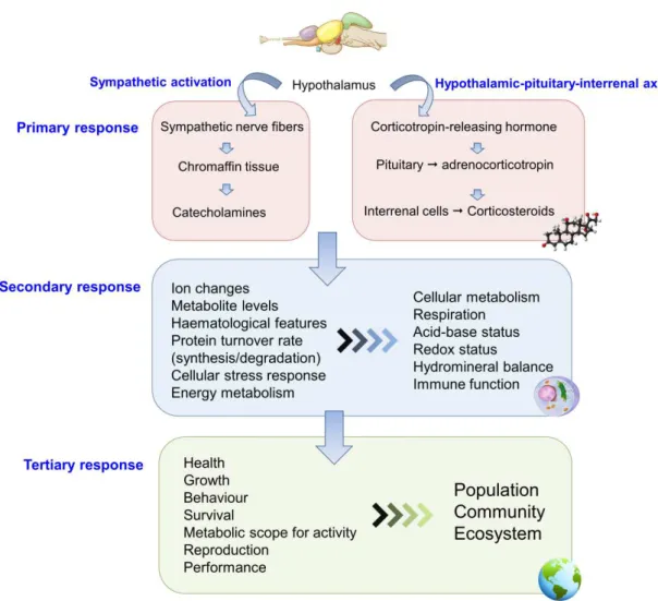
Figure 1.5 Up-scaling of temperature effects from the molecular level to communities and

ecosystems……….8

Figure 1.6 Thermal window and the concept of oxygen and capacity limited thermal tolerance

(OCLTT) (adapted from Pörtner and Farrell, 2008 and Pörtner, 2010). When environmental temperature falls out of the optimum zone, loss of performance starts to take place (at pejus temperatures - Tpejus) due to hypoxaemia caused by a

mismatch of oxygen supply to tissues and the demand for oxygen. At that point, organisms enter the stress zone and several coping mechanisms can be activated, including physiological and molecular adjustments. When the thermal limits are reached (Tcritical), performance is severely affected due to protein denaturation, tissue damage and loss of cellular function. Beyond that temperature point,

(26)

and is based on the action of 3 enzymes, E1, E2 and E3. Ubiquitin-activating enzyme (E1) binds to ubiquitin via a thio-ester bond. This allows for the subsequent step to take place and thus ubiquitin is transferred to the ubiquitin-conjugating enzyme (E2). Following, ubiquitin-ligase (E3) recognizes the protein substrate and catalyzes the transfer of ubiquitin to that substrate. After multiple cycles, the protein substrate is polyubiquitinated and can be linked to the proteasome subunit for degradation of the misfolded protein (peptide bond hydrolysis) with subsequent release of reusable free ubiquitin (via deubiquitinating enzyme) (adapted from Glickman and Ciechanover, 2002; Rahimi, 2012; Amm et al., 2014; Cell Signaling Technology Pathways). Note: mono-ubiquitination has also been recognized as a

proteasome degradation signal……….14

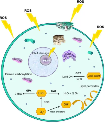
Figure 1.10 Schematic of cellular oxidative damage and anti-oxidant enzyme pathways.

Reactive Oxygen Species (ROS) are enhanced under stressful conditions leading to potential oxidative damage, including DNA deletions and mutations, protein carbonylation and lipid peroxidation. Several enzymes (superoxide dismutase – SOD; catalase – CAT; glutathione peroxidase – GPx; glutathione-S-transferase – GST) counterbalance these effects by catalyzing reactions that transform free

radicals into less toxic or non-toxic products………...16

Figure 1.11 Taxonomy of Sparus aurata………...17

Figure 1.12 Native distribution of the sea bream Sparus aurata (source: Food and Agriculture

Organization of the United Nations)………..17

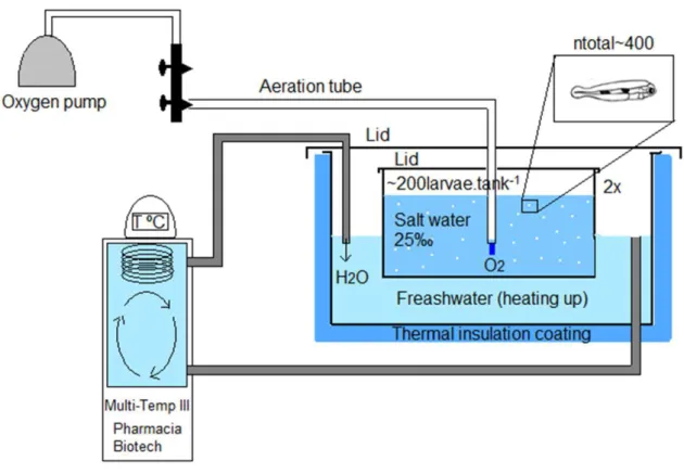
Figure 1.13 Scheme of the thesis workflow………..28 Figure 2.1 Experimental system: two 30L tanks were placed in a thermostatized bath

connected to a heated/refrigerator circulator (MultiTemp III, Pharmacia Biotech). The aquarium was equipped with an aeration system. Both containers (aquarium and thermostatized bath) had a lid to prevent evaporation. The total number of larvae was approximately 400 based on the hatchery’s rounded down estimate of number of larvae per liter. Half of the individuals were transferred to tank 1 and the other half to tank 2 (~200 larvae.tank-1_{). Larvae were obtained from breeding 50}

males with 25 females. Components not to scale………..49

Figure 2.2 Experimental approach (diagram constructed using Experimental Design Assistant,

https://eda.nc3rs.org.uk/)...53

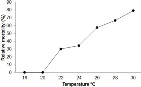
Figure 2.3 Relative mortality of Sparus aurata larvae (12d post-hatch, ≈5mm) along the

temperature gradient (rate of temperature increase of 1ºC.h-1)………54

Figure 2.4 Thermal and oxidative stress biomarkers in larvae (12d post-hatch, ≈5mm) of S. aurata exposed to a temperature gradient (1ºC.h-1) ranging from the control

temperature (18ºC) until the cumulative Critical Thermal Maximum (temperature at which 100% of larvae showed lethargic behavior – 30ºC). a) Hsp70 (Hsc+Hsp70)

and total ubiquitin, b) antioxidant enzymes (glutathione-S-transferase - GST,

superoxide dismutase - SOD, catalase - CAT) and c) lipid peroxidation - LPO and

protein carbonylation – PC. Two pooled samples (comprising of 20 larvae each) were taken at each temperature point. Results are shown as mean±sd. Groups significantly different from control are marked with an asterisk (p<0.05, ANOVA,

Dunnett’s post-hocs)………..……….56

Figure 2.5 Cluster analysis dendrogram (amalgamation rule: single linkage; distance metrics:

1-Pearson r) of all variables measured in S. aurata larvae (12d post-hatch, ≈5mm)

along a temperature gradient (1ºC.h-1_{) ranging from the control temperature (18ºC)}

until the Critical Thermal Maximum (temperature at which 100% of larvae showed lethargic behavior – 30ºC). GST – glutathione-S-transferase; SOD – superoxide dismutase; LPO – lipid peroxidation; TUb – total ubiquitin; CAT – catalase; Hsp70 – Heat shock protein 70kDa; PC – protein carbonylation……….57

Figure 2.6 Dorsal overview of S. aurata larva 12d post-hatch, ≈5mm (longitudinal section).ey)

(27)

disorganization, with the creation of obvious lacunae within fiber. Epon-embedded samples stained with Toluidine Blue. Scale bar: 25 μm………58

Figure 3.1 (a) Breeding scheme carried out in the hatchery (total breeding stock has about

400-600 animals). Sparus aurata is a protandric hermaphrodite species, maturing as

male at about 2 years of age and turning into female at about 3 years of age. Therefore, the males that turn into females are replaced by new males (annual replacement; usually the 200-300 largest of one generation are chosen). Accordingly, the largest 200-300 females are removed. Drawings by N. Kramm retrieved from Archipelagos Wildlife Library; (b) Experimental setup (not to scale).

Re-circulating system (total volume of 2,000L) consisting of six 70L white polyvinyl tanks (35  35  55 cm). The flow rate of clean water in each tank was 300 mL.min

-1_{. Larvae were randomly distributed in smaller plastic containers (17.5}__17.5_₁₅

cm, approximately 4.5 L) placed inside the 70L tanks with water flowing through small punctures. All the tanks were filled with clean and aerated sea water (95-100% O2), with a constant temperature of 18±0.5°C (n=2 tanks), 24±0.5ºC (n=2 tanks) and

30±0.5ºC (n= 2 tanks). Salinity was kept at 35‰ and pH at 8±0.01. Experimental temperatures were maintained using thermostat heaters (TetraTec® HT 100, 100-150L, Tetra Werke, GmbH, Melle, Germany); (c) Timeline of experiment………….75 Figure 3.2 Experimental approach (diagram constructed using Experimental Design Assistant,

Figure 3.3 Current and predicted water temperatures in Portuguese coastal areas and Tagus

estuary. Temperatures are in the range of 16-20ºC in coastal waters and 12-24ºC in the Tagus estuary. According to Miranda et al. (2002) Portuguese waters will undergo a 2-3ºC increase by 2100 leading to temperatures in the range of 19-23ºC in the coastal area and 26-30ºC in estuaries and coastal lagoons………..81

Figure 3.4 Survival curves (solid lines) and 95% confidence intervals (dotted lines) of Sparus aurata larvae exposed to 18ºC, 24ºC and 30ºC for a period of seven days. These

curves were compared through the Log-rank test for trend (Chi square=18.64; df=1; p<0.001). Specific comparisons were carried out using Log-rank Mantel-Cox test (18ºC vs 24ºC - Chi square=4.129, df=1, p=0.04; 18ºC vs 30ºC - Chi square=20.92, df=1, p<0.0001; 24 vs 30ºC - Chi square=12.09, df=1, p<0.0005)………..82

Figure 3.5 Image of the master gel depicting the protein spots detected in Sparus aurata larvae. Annotated spots were those that were differentially expressed between

temperature groups (n=4 larvae in each group, 2 technical replicates, ANOVA, p<0.05). Yellow arrows mark the spots that were successfully identified by mass spectrometry. Only 18ºC and 24ºC were compared because there was 100%

mortality in larvae exposed to 30ºC for 7 days………83

Figure 3.6 Protein expression in Sparus aurata larvae exposed to 18ºC and 24ºC for seven

days. Only 18ºC and 24ºC were compared because there was 100% mortality in larvae exposed to 30ºC for seven days. Data is presented as a heat map with clusters to visualize protein Log2 expression values ranging from green (down-regulated) to red (up-(down-regulated). Columns represent different temperatures while rows represent different proteins (identified by spot number and the correspondent identification by mass spectrometry). Full details concerning protein identification are

given in Table 3.1 and supplementary Table S3.1 (annex 2)………...86

Figure 3.7 Distribution of identified proteins by functional classes according to STRAP v1.5, (a)

biological process, (b) cellular component and (c) molecular function. Detailed

functions are described in supplementary Table S3.2 (annex 2)……….87

Figure 3.8 Functional protein association network retrieved from String (v10) using Homo sapiens as model species. This network is enriched in interactions

(p-value=3.86e-4), mainly between heat shock proteins, cytoskeletal components and cargo transporting. HEBP1 – heme binding protein 1; PSMB3 – proteasome subunit beta type 3; HSPA8 – heat shock 70kDa protein 8; TUBA4A – tubulin alpha 4a; TPM1 – tropomyosin 1; KRT - keratin 8; ARPC2 – actin related protein 2/3 complex subunit 2; MYL1 – myosin light chain 1; GH1 – growth hormone 1; HSP90AA1 – heat shock protein 90kDa alpha; POTEF – POTE ankyrin domain family member F; ACTA1 – actin alpha 1 skeletal muscle; KIF2A – kinesin heavy chain member 2A; IQCA1 – IQ

motif containing with AAA domain 1……….88

Figure 3.9 Summary of the study. Sparus aurata larvae exposed to warm temperatures (control

(28)

heat shock protein 90kDa, IQ motif and AAA domain containing protein), intracellular transport (kinesin, IQ motif and AAA domain containing protein), growth (somatotropin), porphyrin metabolism (heme-binding protein), proteolysis (proteasome subunit, IQ motif and AAA domain containing protein), regulation (POTE ankyrin F), cell-cycle regulation and transcription (IQ motif and AAA domain containing protein). These processes may be important in cell-functioning and survival upon challenging environmental conditions but high levels of mortality suggest that full acclimation may not be achieved. Green arrows () indicate up-regulation and red arrows () indicate down-regulation……….94

Figure 4.1 Experimental setup: the fish were randomly placed in 40.5 l white plastic tanks (n=5

tanks, 30  30  45cm with water from the home tank), which were transferred to a thermostatized bath, connected to a heated/refrigerator circulator (MultiTemp III, Pharmacia Biotech). Each tank had a lid to prevent evaporation and was equipped with an aeration system (10-11 fish.tank-1). Note: not to scale………..110

Figure 4.3 a) Levels of Hsp70 (Hsc+Hsp70) in juveniles of Sparus aurata along a temperature

gradient ranging from the control temperature (18ºC) until the Critical Thermal Maximum (CTmax). Six individuals were sampled at each temperature point except 22ºC in brain). Results are shown as mean + SD. Groups with Hsp70 levels significantly different from control are marked with an asterisk (p<0.05). Hsp70 levels differ significantly between tissues. Gills expressed the highest levels (p<0.001), followed by levels in brain and muscle, which showed equivalent levels. Hepatopancreas (liver and infiltrating pancreatic acini) and intestine showed equivalent amounts of Hsp70 but these levels were lower when compared to other tissues (p<0.001). b) Levels of ubiquitin conjugates in juvenile Sparus aurata along

a temperature gradient ranging from the control temperature (18ºC) until the Critical Thermal Maximum (CTmax). Six individuals were sampled at each temperature point (except 22ºC in brain). Results are shown as mean + SD. Groups with ubiquitin conjugates levels significantly different from control are marked with an asterisk (p<0.05). Ubiquitin conjugates levels differ significantly between some of the tissues. Gills, brain and muscle showed equivalent levels of ubiquitinated conjugates, but showed significant differences from hepatopancreas and intestine (p<0.001). Hepatopancreas (liver and infiltrated pancreatic acini) and intestine showed significant differences, intestine having higher amounts of ubiquitin

conjugates (p<0.01)………..115

Figure 4.4 Representative micrographs of the gills of juvenile Sparus aurata exposed to control

or high temperature. a) Normal structure of the gills at control temperature (18ºC)., b) Gill filament showing a lamellar edema (thick arrow), hyperplasia (arrow head) and hypertrophied chloride cell (thin arrow) (32ºC)., c) Detail of several hyperplasic foci (34ºC)., d) Epithelial lifting of lamellae (34ºC)., e) Convoluted lamellae (arrow) at the Critical Thermal Maximum temperature (35.5ºC) and moderate hyperplasia in the interlamellar space (arrow head). f – filament, l – lamellae, er – erythrocyte, gc –

goblet cell. Scale bars: (a, b, d, e) 25µm; (c)

15µm………..………..117

Figure 4.5 Representative micrographs of the muscle of juvenile Sparus aurata exposed to

control or high temperature. a) Normal structure of skeletal muscle at control temperature 18ºC with striated myocytes (Sm) grouped into fascicles (fc) and surrounded by a sheath of connective tissue. Blood vessels (bv) are evident between fascicles and adjacent to the tegument (T), in which melanin is visible (ml)., b)Muscle at the Critical Thermal Maximum temperature (35.5ºC) showing localized atrophy of muscle fibers probably caused by focal necrosis or autophagy. Scale

bars: 25µm………..118

Figure 4.6 Representative micrographs of the liver of juvenile Sparus aurata exposed to control

(29)

(er) were visible in the parenchyma., b) Fat vacuoles (arrow) and slight hyperemia in hepatic vessels (26ºC), c) Fat vacuoles (thick arrow), hyperemia and melanomacrophage aggregates (thin arrows) (28ºC), d) Fat vacuoles (thick arrow), small necrotic foci in the parenchyma (arrow head) involving hyperemia, micro-hemorrhage and melanomacrophage infiltration (30ºC), e) Moderate hepatocellular alteration (arrow) and melanomacrophage infiltration (34ºC). Note the alteration to hepatocyte size and shape. f) Increased hyperemia and hemorrhage, with hepatocytes clearly more eosinophilic (at the Critical Thermal Maximum temperature

of 35.5ºC) . Scale bars: 25µm……….……….119

Figure 4.7 Representative micrographs of the hepatopancreas of juvenile Sparus aurata

exposed to control or high temperature. a) Normal structure of the pancreas at control temperature (18ºC) consisting of acini composed of highly basophilic acinar cells (ac) (with zymogen granules, zm) arranged concentrically in clusters. Hepatic arterioles (ha) are visible holding few erythrocytes., b) Detail of pancreas at 24-26ºC showing some hyperemia (erythrocytes – er) and leucocytes (arrow)., c) Vacuolization of acinar cells accompanied by hyperemia (28ºC)., d) Detail of lipofuscin-like pigments (arrow) accumulated in acinar cells (30-32ºC) e) Pancreatic tissue at 34ºC with atrophied acini, showing diffuse inflammation and necrosis (arrows)., f) Macrophage infiltration (thick arrow) and hyperemia at the Critical Thermal Maximum temperature (35.5ºC). Lipofuscin-like pigments (thin arrow) and necrotic liver tissue (arrow head) are visible. Scale bars: (a, c, d, e, f) : 25µm; (b):

15µm……….………...120

Figure 4.8 Representative micrographs of observed histopathological alterations in the intestine

of juvenile Sparus aurata exposed to control or high temperatures. a and b) Normal

intestinal architecture (18ºC) consisting of mucosal folds lined internally by microvilli (mv) bearing absorptive cells and goblet cells (gc). Underneath the epithelial layer lays the lamina propria (lp) with scattered lymphocytes (thin arrows in b) inside adjacent lymph vessels., c and d) Atrophy of epithelial cells, lymphocyte infiltration, dilated lamina propria (caused by fluid retention) and hyperemia (arrow) at 34ºC.

Scale bars: (a, c): 25µm; (b, d): 15µm………..………121

Figure 4.9 Summary of the study. Sparus aurata juveniles were subjected to a temperature trial

from 18ºC until the Critical Thermal Maximum. Several organs were sampled for quantification of heat shock protein 70 kDa and total ubiquitin. Following, histopathological analyses were carried out. Results showed that S. aurata is

subjected to protein damage, inflammation, changes in immune responses, cell atrophy and cell death when exposed to high temperatures for short periods. Green arrows () indicate an increase in the targeted biomarker when fish are exposed to increasing temperatures and = indicates no change in relation to the control

temperature (18ºC)……….………...125

Figure 5.1 Experimental setup: the fish were randomly placed in 40.5 l white plastic tanks (n=5

tanks, 30  30  45cm with water from the home tank), which were transferred to a thermostatized bath, connected to a heated/refrigerator circulator (MultiTemp III, Pharmacia Biotech). Each tank had a lid to prevent evaporation and was equipped

with an aeration system (10-11 fish.tank-1). Note: not to

scale……….………137

Figure 5.3 Levels (mean + SD) of antioxidant enzymes measured in several organs of juvenile

Sparus aurata exposed to a temperature ramp of 1ºC.h-1 ranging from control

conditions (18ºC) to the Critical Thermal Maximum (CTmax 35.5±0.5ºC). a)

Catalase activity, b) Glutathione-S-transferase (GST) activity, c) Superoxide

dismutase (SOD) activity. Six individuals were sampled at each temperature point (except 22°C for brain tissue). Groups significantly different from controls are

marked with an asterisk (p < 0.05)………..143

Figure 5.4 Levels (mean + SD) of cytochrome P450 1A (CYP P450 1A) measured in the liver of

juvenile Sparus aurata exposed to a temperature ramp of 1ºC.h-1 ranging from

control conditions (18ºC) to the Critical Thermal Maximum (CTmax 35.5±0.5ºC). Six individuals were sampled at each temperature point. Groups significantly different from controls are marked with an asterisk (p < 0.05)………..144

(30)

each temperature point. Groups with LPO levels significantly different from controls

are marked with an asterisk (p < 0.05)………...145

Figure 5.6 (a) Projection of the biomarkers on the factor plane: representation of the

contribution of each biomarker to factor 1 and 2 of the factor analysis. The biomarkers were measured in response to temperature in different organs of Sparus aurata. (b) Factor analysis (principal components as extraction method) of all

investigated biomarkers in the different tissues analyzed in Sparus aurata along the

temperature trial (all temperatures were included in the analysis). The dashed circles represent the groups that differentiate along the factors: gills differentiate along factor 1 (temperatures of 34 and 36ºC), for which SOD activity was the main contributor; and muscle differentiates along factor 2 (temperatures of 32 and 34ºC),

for which the main contributor was GST activity………..…….146

Figure 6.1 Experimental system and sampling, a) Experimental setup (not to scale).

Re-circulating system (total of 2,000L) with six 70L white polyvinyl tanks (35  35  55 cm) for juveniles of Sparus aurata (n=6 individuals.tank-1). Inflow of clean water in

each tank was 300 mL.min-1_{. All the tanks were filled with clean and aerated sea}

water (95-100% O2), with a constant temperature of 18±0.5°C, 24±0.5°C and

30±0.5°C (n=2 tanks for each temperature). Salinity was kept at 35‰ and pH at 8±0.01. All tanks were provided with a filter (ELITE Underwater Mini-Filter Hagen, 220L.h-1_).

b) Timeline and sampling scheme of the experiment. The fish were

euthanized through cervical transection at day 14, 21 and 28 for collection of muscle. At each time point, four individuals were randomly sampled (2 from each

tank). T – Timepoint in

days……….……….161

Figure 6.3 (a) Cumulative mortalities of Sparus aurata juveniles exposed to 18ºC, 24ºC and

30ºC for a period of 28 days. Data was analysed through Student’s t tests, applying

Bonferroni correction (significance level of 0.05). Asterisks mark significant differences from the control group (18ºC); (b) condition (measured through Fulton’s

K condition index) of juvenile Sparus aurata after 21 days of exposure to 18, 24 and

30ºC. Data was compared via a Kruskal-Wallis test (significance level of 0.05). No significance differences were detected for Fulton’s K condition index among

treatments………...168

Figure 6.4 Representative image of the master gel depicting the protein spots detected in

Sparus aurata juveniles. Annotated spots were those that were differentially

expressed between temperature groups (18, 24 and 30ºC; n=4 individuals in each group, 2 per tank; 2 technical replicates; ANOVA p<0.05) (a) time-point 14 days of

exposure (T14) and (b) time-point 21 days of exposure

(T21)……….169

Figure 6.5 Two-way hierarchical clustering analysis and functional categorization of proteome

data from Sparus aurata juveniles subjected to 18ºC, 24ºC and 30ºC. Heat map

representation of the clustered data matrix in which cells denote the Log2 values of protein normalized volumes. The color scale ranges from green (low expression) to red (high expression). Columns represent different temperatures while rows represent different proteins. Biological functions were listed for proteins in each cluster. (a) Time-point: 14 days of exposure. Two proteins were significantly

regulated at 24ºC i.e. increase in triose phosphate isomerase (TPISB) and a decrease in glycogen phosphorylase (PYGB). At 30ºC, all identified proteins were significantly up-regulated when compared to 18ºC and/or 24ºC with the exception of glycogen phosphorylase, which returned to control levels and one isoform of creatine kinase, which was significantly down-regulated at 30ºC (see supplementaryTable S6.1 for Tukey’s post-hocs). (b) Time-point: 21 days of

(31)

the other identified proteins were significantly up-regulated at 30ºC, when compared to 18ºC and/or 24ºC (see supplementary Table S6.1 for Tukey’s post hocs). HSP71 - Heat shock 70 kDa protein 1; ENOA - Alpha-enolase; KAD1 - Adenylate kinase isoenzyme 1; KCRM - Creatine kinase M-type; CAH1 - Carbonic anhydrase 1; ACT2 - Actin, alpha cardiac muscle 2; HSP7C - Heat shock cognate 71 kDa protein; GDIB - Rab GDP dissociation inhibitor beta; NEC1 - Neuroendocrine convertase 1; TPISB - Triosephosphate isomerase B; KCRT - Creatine kinase, testis isozyme; IF4A2 - Eukaryotic initiation factor 4A-II; PYGB - Glycogen phosphorylase; HSP70 - Heat shock 70 kDa protein; G3P - Glyceraldehyde-3-phosphate dehydrogenase; SAMD9L - Sterile alpha motif domain-containing protein 9-like; G6PI - Glucose-6-phosphate isomerase; TPIS - TrioseGlucose-6-phosphate isomerase (Fragments); DHE3 - Glutamate dehydrogenase, mitochondrial. (c) Comparison between 14 and 21 days

of exposure in terms of percent distribution of proteins into functional classes (at 14

days: total of 21 proteins; at 21 days: total of 14

proteins)………..………176

Figure 6.6 (a) Venn diagram showing shared and exclusively regulated proteins among

temperatures and exposure times (14 days – T14, and 21 days – T21). Proteins common to both temperatures were triosephosphate isomerase, adenylate kinase 1 (up-regulated at 24 and 30ºC), sterile alpha motif domain containing protein 9-like and glucose 6 phosphate isomerase (down-regulated at 24ºC and up-regulated at 30ºC). The four proteins shared between exposure times were heat shock 70kDa protein 1, heat shock cognate 71kDa protein, adenylate kinase isoenzyme 1 and triosephosphate isomerase (which were all up-regulated at 30ºC at both exposure times). NOTE: All redundancies were eliminated in this analysis. HSP71 - Heat shock 70 kDa protein 1; ENOA - Alpha-enolase; KAD1 - Adenylate kinase isoenzyme 1; KCRM - Creatine kinase M-type; CAH1 - Carbonic anhydrase 1; ACT2 - Actin, alpha cardiac muscle 2; HSP7C - Heat shock cognate 71 kDa protein; GDIB - Rab GDP dissociation inhibitor beta; NEC1 - Neuroendocrine convertase 1; TPISB - Triosephosphate isomerase B; KCRT - Creatine kinase, testis isozyme; IF4A2 - Eukaryotic initiation factor 4A-II; PYGB - Glycogen phosphorylase; HSP70 - Heat shock 70 kDa protein; G3P - Glyceraldehyde-3-phosphate dehydrogenase; SAMD9L - Sterile alpha motif domain-containing protein 9-like; G6PI - Glucose-6-phosphate isomerase; TPIS - TrioseGlucose-6-phosphate isomerase (Fragments); DHE3 - Glutamate dehydrogenase, mitochondrial. (b) Protein network analysis carried out

using ClueGo+CluePedia 2.1.7 plugin (from Cytoscape v3.2 platform), to depict interactions between the differentially expressed proteins after 14 and 21 days of exposure to high temperatures (species: Danio rerio; biological process ontology

release date 07092015; GO Tree interval from 3 to 8; GO term pathway selection includes at least 1 gene per cluster; kappa score 0.4.; significant pathways (p 0.05

to < 0.0005 were considered). Red nodes represent proteins unique to T14 and green nodes represent proteins unique to T21. Grey nodes represent shared proteins between T14 and T21. Node size relates to significance and number of

genes associated to that biological

process………178

Figure 6.7 Summary of the study. Sparus aurata juveniles exposed to warm temperatures

(control 18ºC vs 24ºC and 30ºC) modulated about 3% of their muscle proteins. This

molecular plasticity was mainly related to energetic processes, chaperoning, cytoskeletal dynamics, acid-base balance, peptide hormone metabolism, vesicular trafficking and inflammatory processes. Fish seemed more able to acclimate to 24ºC, as opposed to 30ºC, as shown by significantly higher levels of cumulative mortality at this temperature. The mechanisms hypothesized to have the greatest influence on fitness outcomes are highlighted in red. Asterisks indicate significant differences from control (p<0.05). Green arrows indicate up-regulation () and red arrows indicate down-regulation (). T14 – 14 days of exposure; T21 – 21 days of

exposure………..………184

Figure 7.1 (a) Experimental setup (not to scale). Re-circulating system (total volume of

2,000L) with six 70L white polyvinyl tanks (35  35  55 cm). Inflow of clean water in each tank was 300mL.min-1_{. All the tanks were filled with clean and aerated sea}

water (95-100% O2), with a constant temperature of 18±0.5°C, 24±0.5°C and

(32)

samples. T – Timepoint in

days………..197

Figure 7.3 Present and projected temperatures for 2100 (+3ºC) in (a) Portuguese coastal

waters (monthly average sea surface temperature for the main coastal cities from 2011-2015) and (b) estuaries (based on data from the Tagus estuary considering

monthly average temperatures collected from 1978 to

2006)……….………...203

Figure 7.4 Cumulative mortalities of Sparus aurata larvae, juveniles and adults exposed to

18ºC, 24ºC and 30ºC for a period of 28 days. Asterisks mark significant differences from the control group (18ºC). Species illustrations were retrieved from Arias and Drake (1990) and FAO (Food and Agriculture Organization of the United

Nations)………...204

Figure 7.5 Integrated biomarker response index and principal components analysis carried out

for each sampled tissue of Sparus aurata (a) larvae (whole body) and juveniles

(gills, muscle, liver, brain, intestine) and (b) adults (gills, muscle, liver, brain,

intestine) exposed to 18ºC, 24ºC and 30ºC, considering all sampling times (7, 14, 21, 28 days); (c) proportion of variance explained in the first and second

components of the principal components analysis carried out for each sampled tissue of each life stage of Sparus aurata considering all temperatures (18ºC, 24

and 30ºC) and sampling times (0, 7, 14, 21, 28

days)………210

Figure 7.6 Histopathological sections of multiple organs from larval, juvenile and adult Sparus aurata subjected to different temperatures (18, 24 and 30ºC). (A) Muscle of a larva

subjected to 24 ºC for seven days. Note the infiltration of inflammatory cells along the junction between skeletal muscle segments (arrowheads). Bundles of disorganized (atrophied) muscle bundles are also visible (arrows). sn) Skin. Staining: Weigert’s Iron Haemtoxylin + van Gieson. (B) Skeletal muscle of an adult

subjected to 24 ºC for 21 days, revealing diffuse atrophy of skeletal muscle (sk) bundles and inflammatory foci (H&E). The subcutaneous adipose tissue (at) was frequently observed to infiltrate affected muscle (H&E). (C) Section through the optic

lobe of an adult fish exposed to 24 ºC for 21 days, revealing low-moderate diffusion of vacuolation (vc) in the medullar area, likely affecting glial tissue (H&E). (D) Liver (hepatopancreas) of an adult fish subjected to 30 ºC for seven days, with diffuse fat vacuolation (fv) plus inflammation, indicated by hyperaemia and infiltration of inflammatory cells into hepatic tissue (arrow heads). The pancreatic acini are severely affected (arrows), revealing loss of zymogen granules (H&E). Inset: Focus of inflammatory cells (likely melanomacrophages) in the vicinity of pancreatic acini in an adult exposed to 24 ºC for 14 days. Here the acini (ac) still presented a normal structure. Note zymogen granules (zg). PAS-Haematoxylin. (E) Hepatopancreas of

a control (18 ºC) adult fish at 21 days, for comparative purposes. These animals presented the normal architecture of hepatic (hp) and pancreatic tissue (pr), similar to juveniles (H&E). (F) Benign bacterial infection by Chlamydia-like bacteria in the

interlamellar space in gills of a control fish collected at 14 days of exposure. fl) filament; lm) lamella. Note the absence of inflammation. These benign infections were present in virtually all animals, regardless of test of age class (H&E). Scale

bars: 25 µm except C (250

µm)………...213

Figure 7.7 Summary figure. The effects of chronic warming (28 days at 18ºC, 24ºC or 30ºC)

were investigated in S. aurata throughout several stages of its life cycle (larvae,

(33)

sensitive to 30ºC, showing tissue injury and no acclimation potential (confirmed by 0% survival). Nevertheless, as adults inhabit coastal waters they may take advantage of their greater mobility to seek thermal refugia. Therefore, the larval stage is the key developmental stage that will determine the viability of S. aurata

populations in a warming ocean. Note: S. aurata drawings were retrieved from

FAO……….……….218

Annex 3

Figure S6.1 General categories of gene ontology obtained from STRAP v1.5 (T14: 14 days of exposure to warming; T21: 21 days of exposure to warming), (a) biological process,

(34)

(35)

T

ABLE INDEX

Table 1.1 Life history traits of Sparus aurata and commercial importance………19

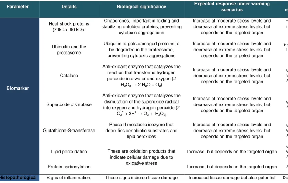
Table 1.2 Parameters used in this thesis, their biological significance and expected results

under warming scenarios……….26

Table 2.1 Sparus aurata life history traits………45

Table 2.2 ANOVA results. Significant results are marked with an asterisk. Hsp70 – heat shock protein 70kDa; Tub – total ubiquitin; LPO – lipid peroxidation; GST – glutathione-S-transferase; SOD – superoxide dismutase; CAT – catalase; PC –

protein carbonylation……….55

Table 3.1 Proteins differentially expressed between temperature groups (18ºC and 24ºC)

in Sparus aurata larvae. Only 18ºC and 24ºC were compared because there was

100% mortality in larvae exposed to 30ºC. These proteins were identified using

MASCOT under the taxonomy Chordata………...84

Table 5.1 One-way ANOVA results for oxidative stress biomarkers for juvenile Sparus aurata exposed to high temperatures. Significant results are marked with an

asterisk (*). GST – glutathione-S-transferase; CAT – catalase; SOD – superoxide dismutase; LPO – lipid peroxidation; CYP450 1A – cytochrome P450

1A.………..142

Table 5.2 Fold-changes induced by high temperature in oxidative stress biomarkers

measured in several organs of Sparus aurata juveniles. CAT – catalase; GST –

glutathione-S-transferase; SOD – superoxide dismutase; CYP1A – cytochrome 1A; LPO – lipid peroxidation.  and  indicate significant fold-changes in relation to controls (18ºC) – temperatures at which these fold-changes occurred are provided below the fold-change;  indicates that the biomarker significantly increased in relation to other groups but not in relation to controls; - indicates no change; N/A non applicable (not performed); variable – there was some variation in biomarker levels but no clear up or down-regulation was detected…………150

Table6.1 Spots differentially expressed between temperature treatments at 14 days of

exposure in the muscle of juvenile Sparus aurata……….170

Table 6.2 Spots differentially expressed between temperature treatments at 21 days of

exposure in the muscle of juvenile Sparus aurata………173

Table 7.1 Variation in biomarker’s levels in comparison to control (18ºC) within each time

point (T7 – seven days of exposure; T14 – fourteen days of exposure; T21 - twenty-one days of exposure). Green arrows () indicate up-regulation and red arrows () indicate down-regulation; hyphen (-) indicates no change in comparison to control (18ºC within that time-point). Hsp70 – heat shock protein 70 kDa; Tub – total ubiquitin; CAT – catalase; GST – glutathione-S-transferase; SOD – superoxide dismutase; LPO – lipid peroxidation………206

Table 7.2 Discriminant function analysis to detect which biomarkers (considering all

organs) contribute to discriminate between life stages (larvae, juveniles, adults), temperature treatments (18, 24 and 30ºC) and exposure times (T7, T14, T21, T28). m – muscle; b – brain; g – gills; l – liver; i – intestine; Hsp70 – heat shock protein 70 kDa; Tub – total ubiquitin; CAT – catalase; GST – glutathione-S-transferase; SOD – superoxide dismutase; LPO – lipid peroxidation………….208 Annex 2

Table S3.1 Masses and sequences of peptides obtained for each spot………243

Table S3.2 Detailed functional categorization of proteins. Information was retrieved from

UniProt, GeneCards, neXtprot beta, InterPro and Qiagen………...……252 Annex 3

Table S6.1 Tukey’s Post-hocs (a) 14 days of exposure, (b) 21 days of exposure…………259 Table S6.2 Protein expression levels extracted from Same Spots concerning the proteomic analysis carried out in the muscle of Sparus aurata exposed to 18ºC, 24ºC and

30ºC for 14 days. Bold lines indicate spots identified through mass

spectrometry……….264

Table S6.3 Masses and sequences of peptides obtained for each spot at (a)14 days of

exposure, (b) 21 days of exposure………...266

Table S6.4 Protein expression levels extracted from Same Spots concerning the proteomic

analysis carried out in the muscle of Sparus aurata exposed to 18ºC, 24ºC and

(36)

information on this table was retrieved from neXtprot, GeneCards, InterPro,

UniProt and Qiagen……….287

Table S6.6 Functional categorization of spots differentially expressed between temperature

treatments at 21 days of exposure in the muscle of juvenile Sparus aurata. The

information on this table was retrieved from neXtprot, GeneCards, InterPro,

UniProt and Qiagen……….291

Annex 4

Table S7.1 Methodology details for laboratorial procedures………297 Table S7.2 Analysis of variance to detect significant differences between biomarker levels

throughout the experiment at the different tested temperatures (18ºC, 24ºC, 30ºC). Significant results are in bold and marked with an asterisk

(37)

(38)

(39)

1. Climate change: global and regional trends

Global average temperatures have been rising over the past century and a half. The Intergovernmental Panel on Climate Change (IPCC, 2014) reports an average increase of 0.85ºC in global temperature since 1880 and refers that the last three decades have been successively warmer (approximately +0.2ºC per decade, Hansen et al., 2006) (Fig. 1.1). This

additional energy is mostly absorbed by the world’s oceans which caused on average a 0.8ºC rise in sea surface temperature over the past 100 years. The scientific community has attributed this warming to human activities, mainly the increase of CO2 and other greenhouse gases in the

(40)

Figure 1.1Global temperature anomalies a) Temperature anomaly for the period of 1980-2014 when compared to the reference period of 1951-1980. The analysis was carried out in Goddard Institute for Space Studies website (NASA, http://data.giss.nasa.gov/gistemp/maps/) following the parameters: data sources land (GISS analysis) and ocean (ERSST_v4); mean period annual; time interval 1980-2014; base period 1951-1980; smoothing radius 1200 km; projection type Robinson. Notes: Gray areas are missing data; ocean data are not used over land nor within 100km of a reporting land station; b) and c) Global ocean and land (respectively) temperature anomalies by year, starting at 1880 until 2014. The right Y axis gives temperature anomaly in degrees Fahrenheit while the right axis is in degrees Celsius (an anomaly of 1ºF is equivalent to an anomaly of 0.556ºC). Source: graphs were obtained using data and tools available in NOAA (National Oceanic and Atmospheric Administration of USA, Department of Commerce, http://www.ncdc.noaa.gov/sotc/global/201509, accessed 16-11-2015).

Global circulation models predict a rise in temperature and changes in ocean chemistry, mostly a decrease in ocean pH (IPCC, 2001, 2007, 2014; Santos et al., 2002). Additionally, changes in climate patterns will escalate extreme events considering their frequency and intensity (heat waves, cold spells, La Niña and El Niño, droughts or heavy rain) (e.g. Fischer and Schär, 2010; IPCC, 2013; Cai et al., 2015). Altogether, such events lead to an altered dynamic of physical and chemical processes, causing a shift in ocean biogeochemistry, hydrodynamics and climate interactions, changes in ocean currents and stratification of ocean waters, a sea level rise (Fig. 1.2), shifts in precipitation patterns, a decrease in ice cover and