Abstract
This paper presents a direct time-domain three dimensional (3D) numerical procedure to simulate the transient response of very large floating structures (VLFS) subjected to unsteady external loads as well as moving mass. The proposed procedure employs the Boundary Element and Finite Element methods (FEM-BEM).The floating structure and the surrounding fluid are dis-cretized by node isoparametric finite elements (FE) and by 4-node constant boundary elements (BE), respectively. Structural analysis is based on Mindlin’s plate theory. The equation of motion is constructed taking into account the effect of inertia loading due to the moving mass. In order to obtain the hydrody-namic forces (added mass and radiation damping), the coupled natural frequencies are first obtained by an iterative method, since hydrodynamic forces become frequency-dependent. Then the Newark integration method is employed to solve the equation of motion for structural system. In order to prove the validity of the present method, a FORTRAN program is developed and numerical examples are carried out to compare its results with those of published experimental results of a scale model of VLFS under a weight drop and airplane landing and takeoff in still water condition. The comparisons show very good agreement.
Keywords
Floating Structure; Finite Element; Boundary Elements; Hydro-dynamic Coefficients; Natural Frequency; Transient response; moving mass.
Time-Domain Three Dimensional BE-FE Method for Transient
Response of Floating Structures Under Unsteady Loads
1 INTRODUCTION
Recently, very large floating structures (VLFS) such as floating airports, floating platforms and floating bridges, have received considerable attention in civil and ocean engineering fields. These
R. E. S. Ismail
Department of Civil Engineering, Beirut Arab University-Tripoli-Branch, Lebanon
(On secondment from Alexandria University, Alexandria, Egypt)
e-mail: ismail_raafat @bau.edu.lb
http://dx.doi.org/10.1590/1679-78251688
tic deformations of VLFS become dominant over the rigid body motions, and the fluid-structure interaction must be included for accurate analysis.
Many researchers have studied the wave-induced hydrodynamic response of floating structures. The wave response of mat-like structure has been studied by a 1D straight-beam and 2D potential flow theory (Wen and Shinozuka, 1972; Suzuki, 1994). Wen (1974) studied the same problem by 2D rectangular plate and 3D potential flow theory. Wang et al. (1995) presented a hydroelastic re-sponse analysis of a box-like floating airport of shallow draft. Hamamoto and Fujita (1995) ana-lyzed the wave response of 3D-module-type floating structure by BE-FE coupled method. Utsunomya et al. (1995) reported the comparison of the results between experimental and theoreti-cal analyses on a mat-type large floating structure. An experimental modal analysis for estimating the dynamic properties of units linked large floating structure model was presented by Endo et al. (1996). Wang and Tay (2010) presented the mathematical formulation for the hydroelastic analysis of pontoon-type VLFS in the frequency domain framework. They employed the coupled finite-element boundary-finite-element (FE-BE) method to solve the coupled water-plate problem. In order to decouple the water-plate interaction problem, they adopted the modal expansion method. Yoon et al. (2014) proposed a direct coupling method to analyze floating plate structures with multiple hinge connections in regular waves. Their method employed finite element method (FEM) and boundary element method (BEM) to discretize floating plates and surrounding fluid, respectively. They investigated the maximum bending moment and deflection in the plate structures.
External unsteady dynamic loads can act on the very large floating airport during landing and takeoff, for example. Such loads will induce the transient behavior of the structure and may affect the safety of landing and taking off. Therefore, the transient hydrodynamic response of VLFS must be clearly clarified.
(2000) proposed a direct time-domain method to analyze the dynamic behavior of flexible floating structure under moving loads. In his method, beam finite elements and two dimension constant boundary elements are employed to discretize the floating structure and the surrounding fluid, re-spectively. Newmark’s method was employed to solve the equation of motion. He considered two types of flexible floating structures, namely: flat type and multiple module-linked bridge structures and studied the effect of stiffness flexibility of the former type and the connector flexibility of the latter type on the dynamic behavior of each type. Cheng et al. (2014) proposed a direct time do-main modal expansion method to compute the transient behavior of VLFS subjected to simultane-ously to incident wave and external loads including weight drop and landing/or takeoff load of an aircraft.
This paper presents a time-domain three dimensional (3D) numerical procedure to simulate the transient response of floating airport subjected to arbitrary unsteady external loads. The proposed method employs the Boundary Element and Finite Element methods (FEM-BEM).The floating structure is discretized by 4-node isoparametric finite element, which is based on Mindlin’s plate theory, whereas the 3D surrounding fluid domain boundaries are discretized by four-node constant boundary elements. The equation of motion takes into consideration the effect of inertia loading due to the moving mass. In order to obtain the hydrodynamic forces (added mass and radiation damp-ing), the coupled natural frequencies are first obtained by an iterative method, since hydrodynamic forces become frequency-dependent. Then the Newark integration method is employed to solve the equation of motion for structural system. Based on the presented procedure, a FORTRAN program is developed and its results are verified by comparison with published experimental results of a scale model of VLFS under a weight drop, airplane landing, and takeoff in still water condition.
2 ANALYTICAL MODEL
The three dimensional floating structure, the coordinate system and the definitions of the fluid domain and boundaries, as shown in Figure 1, are considered in the proposed model. In the present study, the floating structure is assumed to be a plate structure. The plate structure resists exerting forces with bending and torsion moments while the in-plane forces are considered to be negligible. The structure is of constant thickness and linearly elastic. The structure is vertically guided without friction along the sides. The water depth is constant, and is defined as D. The fluid is non-viscous, non-compressible and the fluid motion is irrotational.
2.1 Three Dimension BE Model for Fluid Domain
According to the linear wave theory, the fluid motion can be represented by the velocity potential which can be written as
( , , , )x y z t f e- ⋅ ⋅i w t
F = ⋅ (1)
Figure 1: The floating structure and coordinate system.
The flow velocity, V, can be expressed as:
V = -F (2)
where is the gradient operator. The displacement function of structural motion can be expressed as
i t
i s
uz = ⋅ ⋅e- ⋅ ⋅w (3)
where s is the vertical displacement amplitude.
When a floating structure is vibrating with harmonic motion in the still water, the radiation wave potential can be obtained by solving the Laplace’s equation:
2 2 2
2 0
2 2 2
x y z
f f f
¶ ¶ 
f
¶ ¶ 
= + + =
in Ω
(4-a)
in which Ω is the fluid domain. The boundary conditions at the sea-bed, at sommerfeld’s radiation condition, Dean and Darlrymple (1984), at the free water surface and at the structure-water inter-face are respectively:
0
z
f 
=
lim ( ) 0
r r r i k
f
f
¥
- ⋅ ⋅ =
¶ on G¥ (4-c)
2
z g
f w f
¶ =
¶ on
f
(4-d)
0
x
f
¶ =
¶ on sh (4-e)
s z
f w
= ⋅
¶ on sv (4-f)
in which r=(x2+y2+z2)1/2 is the distance from the origin, to the point to be considered, g is the gravitational acceleration, and k is the wave number given as follows,
2 k g. . tanh( . )k D
w = (5)
where D is the water depth.
The above boundary value problem can be solved by Boundary Element Method (Brebbia, 1989). For this case, weighted residual expression can be written as
* * *
2
( ). .d (q q). .d ( ). .q d
q
f f f f f
f
W = - G - - G
ò ò ò
W G G (6)
in which, q =¶f ¶/ n, ϕ* is weighted function, q*=¶f*/¶n, = ϕ + q, n is the unit normal
vector and the terms with bars, fandq, represent known values of the function and its derivatives.
The inverse formula for Equation (6) is derived as follows,
* * * * *
2
( ). .d ( .q q. ).d ( .q q. ).d
q
f f f
f f f
f
W = - G + - G
ò ò ò
W G G (7)
The fundamental solution ϕ* which is satisfying Equation (8) is adopted solution as weighted
function,
2f* d( , )P Q
= - (8)
where δ(P,Q) is Dirac delta function.
Consequently, by using relation Equation (8), the integral equation (7) is rewritten as follows,
* * * *
( )Q ( ( )q P ( , )P Q q ( , ))P Q d ( ( )P q ( , )P Q q ( , ))P Q d
q
f f f f f
f
= ò ⋅ - ⋅ G - ò ⋅ - ⋅ G
G G (9)
1 *( , ) 4 P Q R f p = (10)
where R=[(xP-xQ)2+(yP-yQ)2+(zP-zQ)2]1/2 is the distance from the point P(xP,yP,zP) of application of
the delta function to any point under consideration, Q(xQ,yQ,zQ).
Incorporating Equation (10) into Equation (9), integral equation on boundary may be derived as follows.
{
* *}
( ) ( ) ( ) ( , ) ( ) ( , )
c P fP q Q f P Q fQ q P Q d
G
⋅ =
ò
⋅ - ⋅ G (11)in which c(P) is constant relating boundary . For a smooth boundary, c(P) =1/2.
The boundary is assumed to be divided into N constant quadrilateral elements. The values of ϕ and q are assumed to be constant over each element and equal to the value at the mid-element node. Then Equation (11) reduces to the following representation before applying any boundary conditions,
1 * *
( ) ( ( , ) ) ( ( , ) )
2 1 1
N N
P q P Q d j P Q d q j
j j
j j
f + å ò ⋅ G ⋅f = å ò f ⋅ G ⋅
= G = G (12)
in which j is the boundary of jth element.
Now, collocation method is adopted to Equation (12) for each element’s mid-point Pi( i=1, 2,...
N)
1 1 1
1 1
2 2 2
1 1 1 1 1 ( ) 2 1 ( ) 2 ... ... ... 1 ( ) 2 N N
j j j j
j j
N N
j j j j
j j
N N
N Nj j Nj j
j j
P H G q
P H G q
P H G q
f f f f f f = = = = = = ìïï
ï + =
ïï ïï ïï
ï + =
ïïí ïï
ï + =
ïï ïï
ï + =
ïï ïïî
å
å
å
å
å
å
(13) in which * ( , ) ,... ... *( , ) ... ...H q P Pi j d when i j
ij j H
ij
H q P Pi i d when i j
ii
i
ìï = ⋅ G ¹
ï ò ò
ïï
ï G
ï = í
ïï = ò ò ⋅ G =
ïï
ï G
ïî
and
*( , )
G P Pi j d
ij
j
f
=ò ò ⋅ G
The integrals can be calculated by using a 4-points Gauss quadrature role for all elements ex-cept the one corresponding to the node under consideration. For this particular case, H
iiis zero due
to the orthogonality of R and n. The boundary integral G
iican be calculated as
1 *( , )
G P Pi i d d
ii R
i i
f
= ò ò ⋅ G = ò ò ⋅ G
G G
2
1 1
2
2 Ai/b ln b b 1 bln b
b
ì é ù ü
ï ï
ï é ù ê + + úï
ï ï
= D íï ê + + ú+ ê úýï
ê ú ê ú
ë û
ï ê úï
ï ï
î ë û þ
(14)
where Ai and b are the area and aspect ratio of the i-th element, respectively.and
(
)
2(
)
2(
)
2R xp xq yp yq zp zq
æ ö÷
ç ÷
ç
= ç - + - + - ÷
÷÷
çè ø
The sea bed boundary, b, radiation boundary, G¥, free surface boundary, f , and structural
boundaries, sh and sv , are numbered as 1, 2, 3, 4 and 5, respectively.
Substituting boundary conditions from equation (4-a) to equation (4-f), into equation (13), equation (13) can be written in matrix expressions as follows:
[ ] { }H ⋅ f =w⋅ ⋅s [ ]G (15)
where,
2
11 12 12 13 13 14 15
2
21 22 22 23 23 24 25
2
31 32 32 33 33 34 35
2
41 42 42 43 43 44 45
2
51 52 52 53 53 54 55
ik
H H G H G H H
g
H H ikG H G H H
g
H H H ikG H G H H
g ik
H H G H G H H
g ik
H H G H G H H
g w w w w w é ù
ê - - ú
ê ú
ê ú
ê ú
ê - ú
ê - ú
ê ú
ê ú
ê ú
é ù = ê - - ú
ë û ê ú
ê ú
ê ú
ê - - ú
ê ú
ê ú
ê ú
ê - - ú
ê ú
ê ú
ë û
(16)
{ }f = êëéf1 f2 f3 f4 f5ùúûT
and (17)
[ ]G = êëéG15 G25 G35 G45 G55ùúûT (18)
2.2 FE Model for Structure
The structure is discretized by 4-node isoparametric finite elements on the basis of Mindlin’s plate theory. The linear equation of motion of structure is given by
{ }
{ }
{ }
{ }
{
( , , )}
gg g g g g g g
F x y t Mst uz Cst uz Kst uz Fr ext
æ ö÷
ç
é ù +é ù +çé ù ÷ = +
ë û ë û çèë û ÷ø (19)
where [Mst] g
, [Cst] g
, and [Kst] g
, are (3NPx3NP) global structural mass, damping and stiffness ma-trices, respectively; {uz}
g
is (3NPx1) global nodal vertical displacement vectors; {Fr} g
is (3NPx1) fluid force vector due to structural motion in the still water; {F(x,y,t)ext}
g
is (3NPx1) time-dependent global external moving load, and NP is total number of nodal points. An over dot on uz
denotes time derivatives.
For Mindlin’s plate bending element, the stiffness matrix [k]e (12x12) is given by
e T T
k Bb Db Bb J d dx h Bs Ds Bs J d dx h
é ù = òòé ù é ù é ù ⋅ +òòé ù é ù é ù ⋅
ë û ë û ë û ë û ë û ë û ë û = éëkbûù+éëksùû (20)
in which [Bb] (3x12) and [Bs] (3x12) are the strain-displacement relationship matrices for bending
and shear deformation, respectively, [Db] (3x3) and [Ds] (3x3) and are the stress-strain relationship
matrices for bending and shear deformation, respectively, [kb] (12x12) , [ks] (12x12), are bending and
shear matrices, respectively and J is Jacobian. To avoid the shear locking phenomenon, a selective reduced integration technique is used. The (2x2) and (1x1) Gauss quadrature is used for bending and shear matrices, respectively. Six Gauss points are used through plate thickness. The element mass matrix[m]e (12x12) is given by
e T
m rst h A N N J d dx h
é ù = ⋅ ⋅òò é ù é ù ⋅
ë û ë û ë û (21)
where, h is the plate thickness, ρst is the mass density of the structure, [N] is the matrix of shape
function. The matrix of shape function used here is defined as: Owen and Hinton (1980).
1 2 3 4
N N N N N
é ù = é ù
ë û ë û (22)
where N1, N2, N3,and N4 have the following expressions:
(
)(
)
1
1 1
1 4
N = +x +h
(
)(
)
1
1 1
2 4
N = -x +h
(
)(
)
1
1 1
3 4
N = -x -h
(
)(
)
1
1 1
4 4
N = +x -h
The time-dependent external force vector {F(x,y,t)ext}g can be impulsive and/or moving loads.
In the case of moving load, there are two models frequently used in the literature (Wu et al., 2000; Esen, 2013): the moving force model and the moving mass model. In the former model, the force is assumed to be constant and equal to the weight of the moving body,
{
F x y t ext( , , )}
g =M g. .d(
x -v t. .) (
d y-e)
(24)where {F(x,y,t)ext} g
is the net force applied by the moving mass on x,y point at time t. δ(x-v.t) and
δ(y-e) represents the Dirac delta functions in x and y directions, respectively, e is the location of the moving mass in y direction, M is the moving mass and v is the moving mass velocity. This model is called inertia-free loading. In the moving mass model, the inertia forces arising due to combined oscillation of this load and the beam (inertial loading) should be considered. In this case, the global external load vector is expressed as
{
( , , )}
. z( , , ) .(
. .) (
)
g
M g x y t x v t y e
F x y t ext = éë -u ùûd - d - (25)
The element nodal forces due to moving mass over the element can be expressed as
(
x y t, ,)
e N T. . .M g(
x v t. .) (
y e)
.J d dFext d d x h
é ù =ò ò é ù - - ⋅
ë û ë û
(
) (
)
. . . .
T
N M N d x v t d y e J d dx h
é ù é ù
-òò ë û ë û - - ⋅
(26)
2.3 Evaluation of Hydrodynamic Force
Since the plate finite element and constant boundary element are used, structure and fluid nodes do not coincide at this stage (Hamamoto and Fujita, 1995). To allocate the fluid force to interface nodes of each finite element, the hydrodynamic pressure on each interface boundary element is re-lated to the plate element nodes by making use of shape function [N] of plate element. The con-sistent fluid force vector at connecting nodes of each plate element can be obtained as
{ }
e TN J d d
fr = òò ë ûé ù ⋅P z⋅ x h (27)
where Pzis the hydrodynamic pressure acting on the central point of each interface boundary
ele-ment given as
. .g
Pz rw t rw uz
¶F
= -
-¶ =i. .wrw. .je-i. .wt-rw. .guz (28)
where ρω is the mass density of sea water. Thus equation 27can be rewritten as
{ }
f e N T(
i. . . . i. .t . .g)
.J d de uz
The radiation wave potential ϕ may be expressed as
Re Im
j = é ùë ûj + é ùë ûj (30)
where Re[ϕ] and Im[ϕ] represent the real and imaginary parts of ϕ, respectively. Incorporating equation 30 into 29 yields
{ }
.(
Re( )
(
. .)
Im( )
(
. .)
)
.. .
e T i t i t
N i g J d d
fr =rwòò ë ûé ù j we-w - j we- w - uz x h
{ }
{ }
{ }
e e e e e e
mw uz cw uz kw uz
é ù é ù é ù
= -ë û -ë û -ë û
(31)
where
{ }
uz e,{ }
uz eand{ }
uz e are the element nodal vertical displacement, velocity and accelera-tion vectors, respectively; [mw]e, [cw]e, and [kw]e are the element matrices of hydrodynamic addedmass, hydrodynamic radiation damping, and hydrostatic stiffness, respectively, and are given by
Re .
.
e w T
N N J d d
mw rws j x h
é ù = òòé ù é ù é ù
ë û ë û ë û ë û (32)
Im .
e w N T N J d d
cw rs j x h
é ù = òòé ù é ù é ù
ë û ë û ë û ë û (33)
. .
e T
g N N J d d
kw rw x h
é ù = òòé ù é ù
ë û ë û ë û (34)
Incorporating equation 31 into equation 19 yields
{ }
{ }
{ }
{
( , , )}
g g g g g g g g g
Mst Mw uz Cst Cw uz Kst Kw uz
g F x y t ext
æ ö÷ æ ö÷ æ ö÷
çé ù +é ù ÷ +çé ù +é ù ÷ +çé ù +é ù ÷
çë û ë û ÷ çë û ë û ÷ çë û ë û ÷
ç ç ç
è ø è ø è ø
=
(35)
where [Mw] g, [Cw] g, and [Kw] g, are the global matrices of [mw] e, [cw] e, and [kw] e, respectively.
Generally, all structures are slightly damped due to structural damping. Due to difficulty in quantifying the structural damping matrix, artificial linear viscous damping is usually added such that [Cst]
g
can be modified to
g g g
Cst aMst b Kst
é ù = é ù + é ù
ë û ë û ë û (36)
where and are called Rayleigh coefficients and given by
1
1 / 1 1 1
2
1 / 2 2 2
a w w h
b w w h
-ì ü é ù ì ü
ï ï ï ï
ï ï= ê ú ï ï
í ý ê ú í ý
ï ï ê ú ï ï
ï ï ï ï
where ωi is the i-th dry mode frequency and ηi is the damping ratio. In this study, it is assumed
that η1= η2= η.
By disregarding the damping terms and external force vector in equation 35, the undamped free vibration of floating structure may be governed by
{ }
{ }
{ }
0g g g g g g
Mst Mw uz Kst Kw uz
æ ö÷ æ ö÷
çé ù +é ù ÷ +çé ù +é ù ÷ =
çë û ë û ÷ çë û ë û ÷
ç ç
è ø è ø (38)
The frequency equation of Equation 38 may be given by
{ }
2 0
g g g g
Kst Kw w Mst Mw
æ ö÷ æ ö÷
çé ù +é ù ÷- çé ù +é ù ÷ =
çë û ë û ÷ çë û ë û ÷
ç ç
è ø è ø (39)
where w is the wet-mode circular frequency of the structure. As the added mass matrix is depend-ent on natural frequency, an iterative solution is carried out to obtain the coupled circular natural frequencies and mode shapes. The initial values are assumed by setting [Mw]
g
= [0] in equation 39. As a result, the element added mass and radiation damping matrices could be obtained by using w
in place of w.
The equation of motion, Equation (35), can be written at time t+ t as:
{
}
{
}
{
}
{
(
)
}
( ) ( )
, ,
( )
g g g g g g
t t t t
Mst Mw uz Cst Cw uz
g
g g g
F x y t t
t t
Kst Kw uz ext
æ ö÷ æ ö÷
çé ù +é ù ÷ + D +çé ù +é ù ÷ + D
çë û ë û ÷ çë û ë û ÷
ç ç
è ø è ø
æ ö÷
ç é ù é ù
+ç ëçè û +ë û ÷÷ + D = + D
ø
(40)
The above equation is a second order differential equation with respect to time, and may be solved by the finite difference method. Newmark’s δ method is adopted here with choosing the value of δ equal to 1/4. This value corresponds to assume constant variation of acceleration during the time increment t. With the aid of this method, the velocity and the acceleration at time t+ t can be expressed in terms of time t as:
{
}
{
}
{
}
{
}
{
}
{
}
{
}
{
}
{
}
2 ( ) ( ) ( ) ( ) 4 4 ( ) ( ) ( ) ( ) ( ) 2g g g g
t t t t t t
uz t uz uz uz
g g g g g
t t t t t t t
uz uz uz t uz uz
t
æ ö÷
ç
= -
-+ D D ççè + D ÷÷ø
æ ö÷
ç
= - -
-+ D ççè + D ÷÷ø D
D
(41)
Substituting Eq. (41) into Eq. (40), the equation of motion of the whole structure is derived as:
{
}
{
( )}
{ }
g g g
K uz t t F
é ù + D =
ë û (42)
{ }
{
(
)
}
{
}
{
}
{
}
4 2
* * *
2
4 * 2 *
, , ( )
2
4 * * *
( ) ( )
*
g g g
g
K K M C
t t
g g
g
g g
F x y t t
F M C uz t
ext t
t
g g g g g
t t
M C uz M uz
t
g g g
K Kst Kw
é ù é ù é ù
é ù = ê ú + ê ú + ê ú
ë û ë û ë û D ë û
D
æ ö÷
ç é ù é ù ÷
ç
= + D +çç ëê úû +D êë úû ÷÷÷
÷
çèD ø
æ ö÷
ç é ù é ù ÷ é ù
ç
+ççD êë ûú +êë úû ÷÷÷ +ëê úû
çè ø
æ
é ù =ç é ù +é ù
ê ú ç ëçè û ë û
ë û
*g g g
M Mst Mw
ö÷÷ ÷ø
æ ö
é ù =ç é ù +é ù ÷÷
ê ú ç ëçè û ë û ÷ø
ë û
*g g g
C æCst Cw ö
é ù =ç é ù +é ù ÷÷
ê ú ç ëçè û ë û ÷ø
ë û
(43)
Equation (42) is the simultaneous linear equations, and can be solved easily to obtain the struc-tural displacement vector {uz (t+Δt)}
g
. Then, the structural velocity and acceleration vectors at time t+ t are calculated by using equation (41).
3 NUMERICAL SIMULATIONS AND RESULTS
In order to validate the proposed time-domain FE-BE hybrid method for analysis of transient elas-tic responses of a floating structure under unsteady external loads, a scale model of Mega-Float is considered with length (L) of 9.75 m, breadth (B) of 1.95 m, thickness (h) of 0.053 m, draft (d) of 0.0163 m, bending stiffness (EI) of 17530 N.m2, and Poisson ratio of 0.3. Based on this scale model, Endo and Yago (1999) carried out experiments under three loading conditions- weight drop test, weight pull-up test, and weight moving test which idealize the airplane landing and takeoff. The tested model called VL-10 in which the plate is floated on the free surface of a towing tank of length 40 m, width 27.5 m and water depth 1.9 m. In these experiments, the vertical displacement at Z1-Z9 points (equally spaced along the central line) as indicated in Figure 1 were measured. For numerical calculations, the dimensions of fluid domain are taken as 30x3x1.9 m, the mass density of water (ρw) is 1x10³ (kg/m3), and mass density of the structure (ρst) is 315.6 (kg/m3). The floating
plate is discretized by 4-node Mindlin’s plate elements with selective reduced integration scheme. It should be noted that when a law order Mindlin’s plate bending element with selective reduce inte-gration technique is used to discretize the plate structure resting on elastic base, the hourglass mode may occur. To avoid this mode to be occurred, two elements with full integration (2x2) is used.
Suzuki and Yoshida (1996) proposed a characteristic length λc, Eq. (44), as a rational measure
1 4 2 EI
c
kc
p
l = æççççè ö÷÷÷÷÷ø (44)
where kc is the spring constant of hydrostatic restoring force. λc, corresponds to the length of locally
deflected region by a static concentrated load. This indicates that the influence of an applied load on the elastic deformation is limited within the region of the length λc.Accordingly, if the length of
structure is smaller than the characteristic length, the response is dominated by rigid-body motions, whereas if it is larger than the characteristic length, as typically in VLFS, the response is dominat-ed by elastic deformations. For the testdominat-ed model, λc = 6.14 m which is less than the plate length,
9.75m. Thus, the response is dominated by elastic deformations.
3.1 Simulation for the Weight Drop Test
The weight drop test is considered here as a typical impulsive experiment. In this test, a weight of 196 N was dropped from a height of 0.12 m onto the “Impact point” indicated in Figure 1 (15 cm a head of point Z2). The detected acceleration of the weight during the impact was recorded, and the result is shown in dimensionless form as the ratio of the gravitational acceleration g in Figure 2. Therefore, this dimensionless acceleration multiplied by 196 N is regarded as the impact load.
As the numerical results may be influenced by the finite element mesh, constant damping ra-tion, η, time increment, Δt, the convergence analysis has to be carried out to obtain best compari-son with the experimental data. The influence of each factor on the accuracy of the numerical simu-lation will be studied in the following sub-sections.
Figure 2: Detected acceleration of weight during impact onto plate.
3.1.1 Effect of Finite Element Mesh
Figure 3: FE Mesh used for discretizing the structure and BE mesh used for discretizing the bounries of fluid domain.
In all considered models, a constant damping ratio, η, is assumed as 0.005 and time step, Δt, is taken as 0.002 s. Figure 4 shows the comparison between the experimental data of the vertical dis-placement time history at point Z1 and the numerical results obtained for various finite element meshes. It can be noticed that the number of elements per structure length (or per characteristic length) significantly influences the accuracy of the numerical results where the accuracy improves with the increase of number of elements. Further, it is observed that when number of elements in-creased from 32 to 64, there is no further improvement in the accuracy. Therefore, the mesh 32x6 will be used in the subsequent analysis.
Figure 4: Influence of finite element mesh.
3.1.2 Effect of Structure Damping Ratio
be noticed that the damping ratio slightly influences the accuracy of the numerical results though the case with damping ratio of 0.005 gives better numerical results in a comparison with experi-mental data. Therefore, a value of 0.005 will be assumed in the subsequent simulations.
Figure 5: Influence of structure damping ratio.
3.1.3 Effect of Time Step
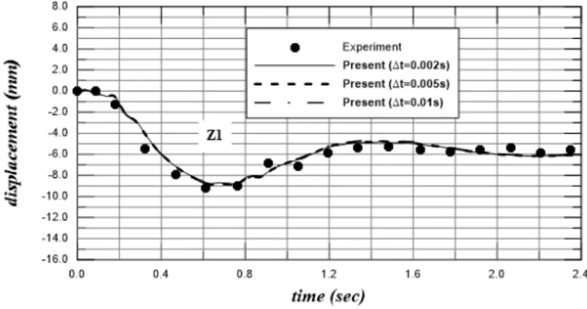
In order to quantify the time step, Δt, three values of time step are considered which are 0.002s, 0.005s, and 0.01s. In all considered models, the plate is discretized by 32x6 (4-node) Mindlin’s plate elements with selective reduced integration and the structure damping ratio, η, is assumed as 0.005. Figure 6 shows the comparison between the experimental data of the vertical displacement time history at point Z1 and the numerical results obtained for various values of time step. It can be noticed that the time step doesn’t influence the accuracy of the numerical results as long as time step is taken less than 0.01s. Therefore, a value of 0.002 will be taken in the subsequent simulations.
Figure 6: Influence of time step.
time step, Δt, is taken as 0.002 s. The comparisons of vertical displacement time history at five measured points with experimental data are indicated in Figure 7. It can be seen from this figure that the present method can predict the global behavior reasonable well. By comparison with the measurements, one can notice that the displacements near the impact point, Z2 and Z1 are larger than the numerical results. This may be attributed to the difference in the effective area of the im-pact load between the experiment (the effective area is infinite) and the numerical simulation (the load is applied at one node which cause the deformation to be localized at the impact point). As it can be observed, the maximum displacement is found at the end z1 and at the point Z2 which are near to the impact point. This can be attributed to the local elastic deformations. Also, one can notice that the transient phenomena can be seen even at time t=1.2s. However, the deformation at t=1.8 s is almost the same as that in static equilibrium
(a)
(b)
Figure 7: Time history of vertical displacement in weight drop test.
3.2 Simulation for the Weight Pull-Up Test
above convergence analysis, the plate is discretized by 32x6 4-node Mindlin’s plate elements with selective reduced integration, a constant damping ratio, η, is assumed as 0.005 and the time step,
Δt, is taken as 0.002 s. The comparisons of vertical displacement time history at five measured points with experimental data are shown in Figure 8.
(a)
(b)
Figure 8: Time history of vertical displacement in weight pull-up test.
As observed in the figure, the calculated results are found to show a good agreement with the experiment. Also, the figure tells us that at almost same time (t= 0.8s) the points Z1, Z2, and Z3 deflect up while the center point Z5 deflects down. However, the deformation at t=2.5 s is almost the same as that in static equilibrium. The end point Z9 raise up at t=1.s before it sinks at t=1.8s though the magnitude of its deflection is small. These findings may be due to that the response is dominated by the elastic deformations.
3.3 Simulation for the Weight Moving Test
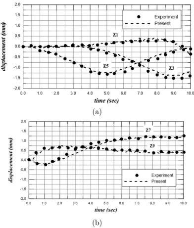
points with experimental data are shown in Figure 9. As observed from the figure, the whole fea-tures are similar to the experimental data. Further, it can be seen that, while the point Z7 deflects down the end point Z9 deflects up. Also the other end point Z1 deflects up while the point Z3 de-flects down. These can be attributed to the fact that the response is dominated by elastic defor-mations. The maximum deflection is found at Z3 and equal to 1.5 mm which is very small com-pared to the plate length.
(a)
(b)
Figure 9: Time history of vertical displacement in weight moving test.
4 CONCLUSIONS
1)The number of elements per characteristic length significantly influences the accuracy of the numerical results. Therefore, a convergence analysis for the element mesh should be carried out at a preliminary stage to identify the size of the finite element to be used in the final simulation.
2)The structure damping ratio has slight influence on the response of the studied floating plate. 3)The time step has insignificant influence on the response as long as its value is taken less
than 0.01s.
4)The numerical results of the proposed procedure are in very good agreement with published experimental results on a rectangular floating structure subjected to external transient loads as well as moving mass.
5)The present method can be extended to study the dynamic response of floating structures with various shapes and end conditions under moving vehicles and/or incident waves. Fur-ther study can be carried out to investigate the effect of various parameters on the hydro-dynamic behavior of such structures.
References
Brebbia, C.A. and Dominguez, J. (1989). Boundary Elements, Computational Mechanics Publications, Southampton, 45-69.
Cheng, Y., Zhai, GJ. and Ou, JP. (2014). Direct time domain numerical analysis of transient behavior of a VLFS during unsteady external loads in waves condition, Abstract and Applied Analysis, 1-17.
Dean, R.G. and Dalrymple, R.A. (1984). Water Waves Mechanics for Engineers and Scientists, Printice-Hall, New York.
Endo, H. (2000). The behavior of a VLFS and airplane during take-off/landing run in wave conditions, Marine struc-ture, 13, 477-491.
Endo, H. and Yago, K. (1999). Time history response of a large floating structure subjected to dynamic load, Journal of the Society of Naval Architect of Japan, 186, 369-376.
Endo, R., Hamamoto, T., Kato, T., Wakui, K. and Imai, T. (1996). Experimental Modal Analysis by Harmonic Sweep Excitation on Unit Linked Floating Models, Proc. of 6th ISOPE, 3, 341-348.
Esen, I. (2013). A new finite element for transverse vibration of rectangular thin plates under a moving mass, Finite Elements in Analysis and Design, 66, 26–35.
Hamamoto, T. and Fujita, K. (1995). Three Dimensional BEM-FEM Coupled Analysis of Module-Linked Large Floating Structures, Proc. of 5th ISOPE. Vol. 3,392-399.
Ismail, R. E. S. (2000). Dynamic Analysis of Flexible-Floating Structures under moving loads using FE-BE Method, Al-Azhar Engineering Sixth International Conference, September 1-4, 277-287.
Kashiwagi, M. (2000). A time-domain calculation method for transient elastic responses of pontoon-type VLFS, Journal Material Science and Technology, 5, 89-100.
Kashiwagi, M. (2004). Transient responses of a VLFS during landing and take-off of an airplane, Journal Material Science and Technology, 9, 14-23.
Lee, D.H., Choi, Y.R., Hong, SY. And Choi, HS. (2001). Time domain analysis for hydroelastic behavior of a mat-type large floating structure in calm water under dynamic loading by mode superposition method, Journal of the Society of Naval Architects of Korea, 38, 39-47.
Ohmatsu, S. (1998). Numerical calculation of hydroelastic behavior of VLFS in time domain, Hydroelasticity in Marine Technology, 89-97.
Owen, D.R.J. and Hinton, E. (1980). “Finite elements in plasticity: theory and practice”, Pine ridge Pubs: 594 p. Qiu, L. (2009). Modeling and simulation of transient responses of a flexible beam floating in finite depth water under moving loads, Applied Mathematical Modeling, 33, 1620-1632.
Qiu, L. and Liu, H. (2007). Three-dimensional time-domain analysis of very large floating structures subjected un-steady external loading, Journal of Offshore Mechanics and Arctic Engineering, 129 (2), 21- 28.
Suzuki, H. and Yoshida, K. (1996). Design flow and strategy for safety of very large floating structure, Proceedings of Int Workshop on Very Large Floating Structures, VLFS’96, Hayama, Japan, 21-27.
Suzuki, Y. (1994). Numerical Analysis on Movements and Wave Transmission Coefficient of Flexible Floating Struc-ture in Waves, Proc. of International Workshop on Floating StrucStruc-tures in Coastal Zone, Port and Harbor Research Institute, Yokosuka, Japan, 222-233.
Utsunomiya, T., Watanabe, E., Wu, C., Hayashi, N., Nakai, K., and Sekita, K. (1995). Wave Response Analysis of a Flexible Floating Structure by BE-FE Combination Method, Proc. of 5th ISOPE, Vol. 3, 400-405.
Wang, C.M. and Tay, Z.Y. (2010). Hydroelastic Analysis and Response of Pontoon-Type Very Large Floating Struc-tures, Fluid Structure Interaction II: Modeling, Simulation, Optimization, Volume 73 de Lecture Notes in computa-tional Science and Engineering, Springer Science & Business Media, Num. pages 432,chapter, 103-130.
Wang, S., Ertekin, R.C., Stiphout, A.T.F.M. and Ferier, P.G.P. (1995). Hydroelstic-Response Analysis of a Box-Like Floating Airport of Shallow Draft, Proc. of 5th ISOPE, 1, 1995, 145-152.
Wen, Y.K. (1974). Interaction of Ocean Waves with Floating Plate, Proc. of ASCE, 100, EM2, 375-395.
Wen, Y.K. and Shinozuka, M. (1972). Analysis of Floating Plate under Ocean Waves, Proc. of ASCE, 98, No. WW2, 177-190.
Wu, JJ. Whittaker, A. R. and Cartmell, M. P. (2000). The use of finite element techniques for calculating the dy-namic response of structures to moving loads, Computers and Structures, 78, 789-799.