www.hydrol-earth-syst-sci.net/15/3767/2011/ doi:10.5194/hess-15-3767-2011
© Author(s) 2011. CC Attribution 3.0 License.
Earth System
Sciences
Spatial moments of catchment rainfall: rainfall spatial organisation,
basin morphology, and flood response
D. Zoccatelli1, M. Borga1, A. Viglione2, G. B. Chirico3, and G. Bl¨oschl2
1Department of Land and Agroforest Environment, University of Padova, Italy
2Institut f¨ur Wasserbau und Ingenieurhydrologie, Technische Universit¨at Wien, Vienna, Austria 3Dipartimento di Ingegneria Agraria, Universit`a di Napoli Federico II, Naples, Italy
Received: 7 June 2011 – Published in Hydrol. Earth Syst. Sci. Discuss.: 21 June 2011 Revised: 15 October 2011 – Accepted: 17 November 2011 – Published: 20 December 2011
Abstract.This paper describes a set of spatial rainfall statis-tics (termed “spatial moments of catchment rainfall”) quan-tifying the dependence existing between spatial rainfall or-ganisation, basin morphology and runoff response. These statistics describe the spatial rainfall organisation in terms of concentration and dispersion statistics as a function of the distance measured along the flow routing coordinate. The in-troduction of these statistics permits derivation of a simple relationship for the quantification of catchment-scale storm velocity. The concept of the catchment-scale storm veloc-ity takes into account the role of relative catchment orienta-tion and morphology with respect to storm moorienta-tion and kine-matics. The paper illustrates the derivation of the statistics from an analytical framework recently proposed in literature and explains the conceptual meaning of the statistics by ap-plying them to five extreme flash floods occurred in various European regions in the period 2002–2007. High resolution radar rainfall fields and a distributed hydrologic model are employed to examine how effective are these statistics in de-scribing the degree of spatial rainfall organisation which is important for runoff modelling. This is obtained by quan-tifying the effects of neglecting the spatial rainfall variabil-ity on flood modelling, with a focus on runoff timing. The size of the study catchments ranges between 36 to 982 km2. The analysis reported here shows that the spatial moments of catchment rainfall can be effectively employed to isolate and describe the features of rainfall spatial organization which have significant impact on runoff simulation. These statistics provide useful information on what space-time scales rainfall has to be monitored, given certain catchment and flood char-acteristics, and what are the effects of space-time aggregation on flood response modeling.
Correspondence to:D. Zoccatelli ([email protected])
1 Introduction
Rainfall is a highly heterogeneous process over a wide range of scales both in space and time (e.g. Rodriguez-Iturbe et al., 1998; Fabry, 1996; Marani, 2005). Whether or not spa-tial heterogeneity of rainfall has an impact on catchment dis-charge and for what reason, is a problem that has been often addressed in hydrology and that is still poorly understood. Many hydrological studies have focused on the role of rain-fall space-time variability in catchment response, with the aim of developing a rationale for more effective catchment monitoring, modelling and forecasting (e.g. Naden, 1992; Obled et al., 1994; Bl¨oschl and Sivapalan, 1995; Bell and Moore, 2000; Andr´eassian et al., 2001; Morin et al., 2006; Moulin et al., 2008; Saulnier and Le Lay, 2009; Gourley et al., 2011). From a practical perspective, it is important to know at what space-time scales rainfall has to be monitored, given certain catchment and flood characteristics, and what are the effects of space-time aggregations on model simula-tions (Berne et al., 2004).
which directly control the runoff response. In this paper, the rainfall spatial organization is analysed with respect to the flow distance, i.e. the distance along the runoff flow path from a given point to the outlet.
Observational and modelling studies have shown that the river network geometry plays a central role in the structure of the catchment dampening properties, particularly for cases of extreme floods when the impact of land properties het-erogeneity on runoff generation is less significant with re-spect to moderate floods and the stream network extends to previously unchanneled topographic elements, hence in-creasing drainage density and flow response rate of hillslopes (Naden, 1992; Woods and Sivapalan, 1999; Smith et al., 2002; Nicotina et al., 2008; Sangati et al., 2009). Runoff routing through branched channel networks imposes an ef-fective averaging of spatial rainfall excess across locations with equal routing time, in spite of the inherent spatial vari-ability. The flow distance coordinate may be used as a surro-gate for travel time, when the hydrograph response is deter-mined mainly by the distribution of travel times, neglecting hydrodynamic dispersion, and variations in runoff propaga-tion celerities may be disregarded. This implies that rainfall spatial organisation measured along the river network by us-ing the flow distance coordinate may be a significant property of rainfall spatial variability when considering flood response modelling.
Various measures of rainfall organisation based on the flow distance coordinate have been introduced in the last decade. Smith et al. (2002, 2005), Zhang et al. (2001) and Borga et al. (2007), in a series of monographs on extreme floods and flash floods, systematically employed a scaled measure of distance from the storm centroid and scaled measures of rainfall variability to quantify the storm spatial organisation and variability from the perspective of a distance metric im-posed by the river network. Smith et al. (2004a) examined basin outflow response to observed spatial variability of rain-fall for several basins in the Distributed Model Intercompar-ison Project (Smith et al., 2004b), by using, among other in-dexes, a rainfall location index based on the distance from the centroid of the catchment to the centroid of the rainfall pattern. They found that all basins except one had a very limited range of rainfall location index, with the rainfall cen-troid close to the catchment cencen-troid. Interestingly, the catch-ment displaying the largest range of rainfall location index was also the one characterised by such complexities to sug-gest the use of a distributed model approach. A similar ap-proach was taken by Syed et al. (2003) who evaluated the ability of simple geometric measures of thunderstorm rain-fall in explaining the runoff response from a 148 km2 wa-tershed. They also used a location index similar to that in-troduced by Smith et al. (2004a). They observed that the position of the storm core relative to the watershed outlet be-comes more important as the catchment size increases, with storms positioned in the central portion of the watershed pro-ducing more runoff than those positioned near the outlet or
near the head of the watershed. Woods and Sivapalan (1999) proposed an analytical method to identify the importance of different components of the hydrological cycle during storm events in humid temperate catchments. They expressed the mean catchment runoff time as a function of the distance from the centroid of the catchment to the centroid of the rainfall excess pattern measured along the flow distance co-ordinate. This term summarised the influence of the rainfall spatial variability on the timing of the flood peak discharge in their model. However, the extent of potential application of this method is limited by the assumption of multiplicative space-time separability for both rainfall and runoff genera-tion processes. This implies that the storm event is assumed to be stationary, i.e. it does not move over the catchment. This assumption is relaxed in the analytical framework in-troduced by Viglione et al. (2010a), which describes the de-pendence of the catchment flood response on the space-time interactions between rainfall, runoff generation and routing mechanisms. Notably, this method affords examination of the effects of storm movement on runoff properties.
coherent theoretical framework for both hydrologic flow and transport, as shown by Rinaldo et al. (2006).
As part of this analysis, we show how the introduction of the spatial moments of catchment rainfall permits derivation of a simple relationship for the quantification of storm veloc-ity at the catchment scale. The importance of storm move-ment on surface runoff has been investigated for nearly four decades (Maksimov, 1964; Surkan, 1974; Ogden et al., 1995; Singh, 1998; de Lima and Singh, 2002). However, to the best of our knowledge, these works are based on “virtual experi-ments” using idealized storm profiles and motion as input to watershed models. Results seem to support the conclusion that catchment response is sensitive to storm motion relative to catchment morphology, depending on different processes and scales. With this work we show how it is possible to iso-late and quantify the “catchment scale storm velocity”, gen-erated by imposing a prescribed space-time storm variability to the catchment morphological properties.
In the following developments, we disregard the differen-tiation between hillslopes and channel network to the total runoff travel time. While the methodology can be easily ex-tended to include a hillslope term, we prefer here to focus on the interaction between the morphological catchment prop-erties and rainfall organisation. On going investigations are aimed to examine the impact of varying the hillslope resi-dence time on both the spatial moments of catchment rainfall and the catchment scale storm velocity.
The conceptual meaning of the spatial moments is illus-trated by analysing five extreme flash floods occurred in var-ious European regions in the period 2002–2007. High resolu-tion, carefully controlled, radar rainfall fields and a spatially distributed hydrologic model are employed to examine the use of these statistics to describe the degree of spatial rainfall organisation which is important for runoff modelling, with a focus on runoff timing. The size of the study catchments ranges between 36 to 982 km2. Hillslope residence time and
spatial variability of runoff ratio, which are disregarded in the derivation of the spatial moments, are included in the dis-tributed hydrological model. Therefore, contrasting model results with information inferred from the spatial moments provides a necessary evaluation of the impact of the work-ing assumptions on the use of these statistics, at least in the context of extreme floods.
The outline of the paper is as follows. In Sect. 2 we de-fine the statistics termed “spatial moments of catchment rain-fall”. In Sect. 3 we show how these rainfall statistics can be related to the flood hydrograph properties. Section 4 is de-voted to illustrate the derivation of the spatial moments of catchment rainfall for the five flood events. In Sect. 5 we perform numerical experiments in which modelled flood re-sponse obtained by using detailed spatial input is contrasted with the corresponding flash flood response obtained by us-ing spatially uniform rainfall. Runoff model sensitivity to spatial organisation of rainfall is examined by exploiting the
spatial rainfall statistics. Section 6 completes the paper with discussion and conclusions.
2 Spatial moments of catchment rainfall: definitions
Spatial moments of catchment rainfall provide a description of overall spatial rainfall organisation at a certain timet, as a function of the rainfall fieldr(x,y,t )(L T−1) value at any po-sitionx,yinside the watershed and of the distanced(x,y)(L) between the positionx,yand the catchment outlet measured along the flow path. The spatial moments of catchment rain-falls are defined after rearranging some of the covariance terms employed in Viglione et al. (2010a) to represent the mean and the variance of the network travel time, under the hypothesis of constant flow velocity (Appendix). The n-th spatial moment of catchment rainfallpn (Ln+1 T−1) is ex-pressed as:
pn(t )= |A|−1
Z
A
r(x,y,t )d(x,y)ndA (1)
whereA (L2) is the spatial domain of the drainage basin. The zero-th order spatial moment p0(t )yields the average
catchment rainfall rate at timet.
Analogously, thegn(Ln) moments of the flow distance are given by:
gn= |A|−1
Z
A
d(x,y)ndA . (2)
The zero-th order spatial moment of flow distance yields unity. Non-dimensional (scaled) spatial moments of catch-ment rainfall can be obtained by taking the ratio between the spatial moments of catchment rainfall and the moments of the flow distance, as follows, for the first two orders:
δ1(t )=pp0(t )g1(t )1
δ2(t )=
A−1R A
r(x,y,t )[d(x,y)−δ1(t )g1]2dA
A−1R
A
r(x,y,t )dA A−1R
A
[d(x,y)−g1]2dA
= 1
g2−g21
p2(t )
p0(t )−
p1(t )
p0(t )
2
(3)
where for the second order the central moment is reported. The first scaled momentδ1(–) describes the distance of the
centroid of catchment rainfall with respect to the average value of the flow distance (i.e. the catchment centroid). Val-ues ofδ1close to 1 reflect a rainfall distribution either
con-centrated close to the position of the catchment centroid or spatially homogeneous, with values less than one indicating that rainfall is distributed near the basin outlet, and values greater than one indicating that rainfall is distributed towards the catchment headwaters.
The second scaled moment δ2 (–) describes the
Values ofδ2close to 1 reflect a uniform-like rainfall
distri-bution, with values less than 1 indicating that rainfall is char-acterised by a unimodal distribution along the flow distance. As we will see below, values greater than 1 are generally rare, and indicate cases of multimodal rainfall distributions.
The spatial moments defined in Eq. (3) describe the instan-taneous spatial rainfall organization at a certain timet. Equa-tions (1) to (3) can also be used to describe the spatial rainfall organization corresponding to the cumulated rainfall over a certain time periodTs (e.g. a storm event). These statistics,
which are obtained by integrating over time, are termedPn and1n. These statistics are defined as follows:
Pn= |A|−1
Z
A
rt(x,y)d(x,y)ndA= 1 Ts
Z
Ts
pn(t )dt (4)
wherert(x,y)is the mean value of time integrated rainfall at location(x,y). 11 and 12 are computed based on Pn following Eq. (3), as follows
11=PP1
0g1
12= 1
g2−g21
P2
P0−
P1
P0
2 (5)
The distance from the rainfall centroid to the catchment outlet is represented by the productδ1g1.Interestingly, the
analysis of the evolution in time of this distance enables the calculation of an instantaneous catchment-scale storm veloc-ity along the river network, as follows:
Vs(t )=g1 d
dtδ1(t ) (6)
Positive values of the storm velocityVs (L T−1) correspond
to upbasin storm movement, whereas downbasin storm movement are related to negative values of Vs. The
con-cept of the catchment-scale storm velocity defined by Eq. (6) takes into account the role of relative catchment orientation and morphology with respect to storm motion and kinemat-ics. For instance, for the same storm kinematics, the same elongated basin will be subject to different catchment scale storm velocities by varying its orientation with respect to that of the storm motion. In this work, we will not perform any explicit derivative ofδ1to obtain the catchment scale storm
velocity. Equation (6) has been introduced only to formally represent the concept of storm velocity and how this relates to the first scaled momentδ1. A simple way to derive the
mean value ofVs, derived from the methodology introduced
by Viglione et al. (2010a), is reported in the next sections.
3 Relationship between the spatial moments of catchment rainfall and the shape of the flood response
Viglione et al. (2010a) proposed an analytical framework (called V2010 hereafter) for quantifying the effects of space-time variability on catchment flood response. Viglione et al. (2010a) extended the analytical framework developed in Woods and Sivapalan (1999) to characterize flood response in the case where complex space and time variability of both rainfall and runoff generation are considered as well as hills-lope and channel network routing.
In the V2010 methodology, the rainfall excessre(x,y,t )
(L T−1) at a point (x,y)and at timetgenerated by precipita-tionr(x,y,t )is given by
re(x,y,t )=r(x,y,t )·c(x,y,t ) (7)
wherec(x,y,t )(–) is the local runoff coefficient, bounded between 0 and 1. V2010 characterizes the flood response with three quantities: (i) the catchment- and storm-averaged value of rainfall excess, (ii) the mean runoff time (i.e. the time of the center of mass of the runoff hydrograph at a catch-ment outlet), and (iii) the variance of the runoff time (i.e. the temporal dispersion of the runoff hydrograph). The mean time of catchment runoff is a surrogate for the time to peak. The variance of runoff time is indicative of the magnitude of the peak runoff. For a given event duration and volume of runoff, a sharply peaked hydrograph will have a relatively low variance compared to a more gradually varying hydro-graph (see Woods, 1997, for details).
Since the aim of this study is to establish a relationship be-tween the spatial moments of catchment rainfall and the flood response shape, we modified accordingly the V2010 method-ology by assuming that the runoff coefficient is uniform in space and time, and that the hillslope residence time is neg-ligible. Hence, in the following developments the rainfall in-tensity and accumulation are used in place of the rainfall ex-cess. Owing to this assumption, results obtained by this ap-proach are likely to apply to heavy rainfall events character-ized by large rain rates and accumulations. The runoff trans-port is described by using an advection velocityv (L T−1) which is considered invariant in space and time. The hy-pothesis of spatially uniform flow velocity is consistent with the results of previous studies, showing that it is always pos-sible to find a single value of flow celerity v such as the mean travel time across the entire catchment and therefore the catchment response time is unchanged (Robinson et al., 1995; Saco and Kumar, 2002; D’Odorico and Rigon, 2003).
The analytical results are summarized below, by focusing on the elements which are essential to derive the relation-ship between the spatial moments and the characteristics of the flood response shape, i.e. the mean and the variance of runoff time and the catchment scale storm velocity. Catch-ment runoff time is treated as a random variable (denotedTq),
drop of water exits the catchment. Water that passes a catch-ment outlet goes through two successive stages in our con-ceptualisation: (i) the generation of runoff at a point (includ-ing wait(includ-ing for the rain to fall), (ii) runoff transport. Each of these stages has an associated “holding time”, which is con-veniently treated as a random variable (e.g. Rodriguez-Iturbe and Valdes, 1979). Since the water exiting the catchment has passed in sequence through the two stages mentioned above we can write
Tq=Tr+Tc
whereTrandTcare the holding times for rainfall excess and
runoff transport.
Mean catchment runoff time. Using the mass conservation property (see V2010) we can write the mean ofTqas
E(Tq)=E(Tr)+E(Tc) (8)
The first termE(Tr)represents the time from the start of the
event to the centroid of the rainfall time series, and is inde-pendent from the rainfall spatial variability. For the concep-tualization ofE(Tr), which is not of interest here, we refer to
V2010. The second termE(Tc)represents the average time
to route the rainfall excess from the geographical centroid of the rainfall spatial pattern to the catchment outlet. By us-ing the spatial moments, the termE(Tc)may be expressed as
follows:
E(Tc)=
RTs
0
hRA
0 r(x,y,t )d(x,y)dA
i
dt
ATsP0v
= P1 P0v
=11g1
1
v (9)
whereTsis the duration of the storm event.
Therefore, Eq. (8) may be written as follows: E(Tq)=E(Tr)+
11g1
v (10)
Details concerning the derivation of Eq. (10) based on V2010 are reported in the Appendix. It is important to note here that the spatial distribution of the rainfall excess is the same as that of the rainfall pattern, since the runoff coefficient is assumed to be spatially uniform.
It is interesting to note that, from Eq. (10), the first time-integrated scaled moment represents the ratio between the routing time corresponding to the rainfall center of mass with respect to the catchment response timeg1/v:
11= E(Tc)
g1
v
(11) Analogously to δ1, the values of 11 are greater than zero,
and are equal to one for the case of spatially uniform precip-itation or for a spatially variable precipprecip-itation which is con-centrated on the catchment centroid. Values of11less than
one indicate that rainfall is concentrated towards the outlet,
and values larger than one indicate that rainfall is concen-trated towards the headwater portion of the basin. Based on Eq. (10), the statistic11 measures the hydrograph
tim-ing shift relative to the position of the rainfall centroid over the catchment. As it will be shown later in the paper, the statistic11is related to the normalised mean time difference
between the hydrograph obtained by considering the actual rainfall pattern and the hydrograph resulting from a spatially uniform rainfall pattern (all other factors being taken equal). The normalising quantity is given by the response time of the catchment. The effect of a less-than-one value of 11
indicates an anticipation of the mean hydrograph time with respect to the case of spatially uniform precipitation. The opposite holds true for the case of a larger-than-one value of the statistic. As an example, this means that a value of11
equal to 1.5 indicates that the mean time difference between the two hydrographs corresponds to half the catchment re-sponse time, with the hydrograph obtained from the spatially distributed rainfall delayed with respect to the one obtained from uniform rainfall. A value of11equal to 0.5 indicates
the same normalized mean difference, but with the opposite sign (the hydrograph obtained from the spatially distributed rainfall is anticipated with respect to the one obtained from uniform rainfall).
One should note that the storm velocity has no influence on E(Tq). This is a direct consequence of the hypotheses used
to derive the statistics. The catchment response is described as fully kinematic, therefore it is influenced by the averaged spatial organization of the rainfall and not by the variability of the spatial organization within the storm, and the routing is linear.
Variance of catchment runoff time. The variance ofTq,
which represents the dispersion of the hydrograph, is given by
Var(Tq)=Var(Tr)+Var(Tc)+2Cov(Tr,Tc) (12)
We focus here on the terms Var(Tc)and 2 Cov(Tr,Tc). For
the conceptualization of Var(Tr), which is not of interest
here, we refer to V2010.
By using the concept of scaled spatial moments, Var(Tc)
may be written as follows. Var(Tc)=
12 v2
g2−g12
(13) Details concerning the derivation of Eq. (13) are reported in the Appendix, based on V2010. For the case of Cov(Tr,Tc)
equal to zero,12represents the ratio between the differential
variance in runoff timing generated by rainfall spatial distri-bution, and the variance of the catchment response time. The values of12are greater than zero and take the value of one
when the rainfall field is spatially uniform. When the rain-fall field is spatially concentrated anywhere in the basin, the values of12 are less than one. In the less frequent cases
catchment, the values of12are greater than one. It should
be noted that, with the rainfall excess volume remaining un-changed, the effect of decreasing the variance of runoff time is to increase the flood peak. This shows that in general the parameter11is expected to have an influence on the runoff
timing, whereas the parameter12should affect the shape of
the hydrograph and then the value of the flood peak. As discussed in V2010, Eq. (25), the role of catchment scale storm velocity is represented by the term Cov(Tr,Tc).
By using rainfall weights, defined as w(t )=p0(t )
P0
(14) and based on V2010 (see Appendix for the details of the derivation), the term Cov(Tr,Tc)in Eq. (12) may be written
as follows:
Cov(Tr,Tc)=g1
Covt[T ,δ1(t )w(t )]
v
| {z }
term1
−Covt[T ,w(t )]
v
| {z }
term2 11 (15)
where Covt[] is the temporal covariance of the space-averaged terms. Here we define the term “catchment scale storm velocity”Vsas follows
Vs(t )=g1
Covt[T ,δ1(t )w(t )]
var[T]
| {z }
Vs1
−g1
Covt[T ,w(t )] var[T] 11
| {z }
Vs2
(16)
where the two velocity termsVs1andVs2 correspond to the
groups term1and term2in Eq. (15). It is worth recognizing
that the groups term1 and term2 represent the slope
coeffi-cients of linear space-time regressions. Term1 is the slope
coefficient of the regression of the productδ1(t )w(t ) with
time; term2is the slope coefficient of the regression of the
weightsw(t )with time.
Equation (16) shows that the velocity formulation is given by the difference between two velocity terms. The first term describes the total storm motion, as related to the temporal evolution of the product of the weights of the precipitation w(t )and of the centroidδ1(t ). The second term describes the
temporal storm variability, as it is summarized by the tempo-ral evolution of the precipitation weights. Some examples may help understand the concept of storm velocity in ideal-ized cases. For the case of temporally uniform mean areal rainfall,w(t )is constant,Vs2is equal to zero, and the value
ofVsdepends only on the evolution in time of the position of
the rainfall centroid along the flow distance coordinate (Vs1).
Conversely, if there is only temporal variation of the mean areal rainfall andδ1(t )is constant, the two velocity termsVs1
andVs2will be equal in value and opposite in sign, implying
thatVswill be equal to zero. Note that the sign of the velocity
is positive (negative) for the case of upstream (downstream) storm motion.
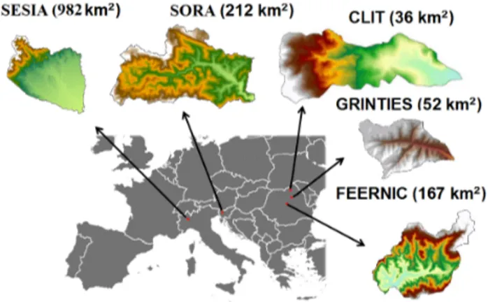
Fig. 1.Study catchments and their location in Europe.
Finally, the term Cov(Tr,Tc)may be written as follows:
Cov(Tr,Tc)=g1
Covt[T ,δ1(t )w(t )]
v
| {z }
term1
−Covt[T ,w(t )]
v
| {z }
term2 11
=Vs
vVar[T]
(17)
As a result, for downstream moving storm the variance of catchment runoff time tends to reduce and therefore the peak discharge tends to increase, consistently with the findings from several investigations (Niemczynowicz, 1984; Ogden et al., 1995; De Lima and Singh, 2002). The opposite oc-curs with upstream moving storms, which tend to increase the hydrograph time variance and hence to reduce the peak discharge.
4 Assessment of spatial moments of catchment rainfall
Europe since 1994, with twenty events occurred since 2000. The hydro-meteorological data includes high-resolution rain-fall patterns, flow type processes (either liquid flow or de-bris flow or hyperconcentrated flows) and hydrographs or peak discharges. Climatic information and data concerning morphology, land use and geology are also included in the database. These data enable the identification and analysis of the hydrometeorological causative processes and the indi-vidual reconstruction of the events by using hydrologic and hydraulic modelling.
For the five events, both original raw radar reflectivity val-ues and raingauge data were made available for rainfall esti-mation. The quantitative precipitation estimation problem is particularly crucial and difficult in the context of flash-floods since the causative rain events may develop at very short space and time scales (Krajewski and Smith 2002; Bouil-loud et al., 2010). The methodology implemented here for radar rainfall estimation is based on the application of cor-rection procedures exploiting the understanding of radar ob-servation physics. It is based on (1) detailed collection of data and metadata about the radar systems and the raingauge networks (including raingauge data from amateurs and from bucket analysis), (2) analysis of the detection domain and the ground/anthropic clutter for the considered case (Pellarin et al., 2002), (3) implementation of corrections for range-dependent errors (e.g. screening, attenuation, vertical profiles of reflectivity) and (4) optimisation of the rainfall estimation procedure by means of radar-raingauge comparisons at the event duration scale (Buoilloud et al., 2010). The methodol-ogy was applied consistently in the same form over the five storm events.
Analyses of rainfall variability by means of the spatial moments is attempted here to isolate and describe the fea-tures of rainfall spatial organisation which have significant impact on runoff simulation. As such, spatial moments pro-vide information to quantify hydrological similarities among different storms, and support the transfer of knowledge and exchange of estimation and analysis techniques. The rain-fall spatial moments and the catchment-scale storm veloc-ity were computed at each time step (either at 15-min or 30-min time steps) as time series, to examine the variabil-ity in time of the statistics. The time series of the first and second scaled moments of catchment rainfall are reported in Plates 1 and 2, together with the basin-averaged rainfall rate, the fractional coverage of the basin by rainfall rates exceed-ing 20 mm h−1 (this threshold has been selected to indicate
a flood-producing rainfall intensity), and the storm velocity. The values of catchment scale storm velocity were computed by applying Eq. (16). The two velocity termsVs1 andVs2
were computed by assessing the slope of the corresponding linear regressions, by using a moving window with window size equal to the catchment response time.
The time series of the first scaled spatial momentδ1exhibit
a relatively large variability, particularly in the Feernic case, with the first scaled moments varying from 0.6 to 1.6 in the
first 80 min (with a clear upbasin storm motion, as reflected in the increasing values of the statistic) and then decreasing in the following three hours, where a downbasin storm mo-tion can be recognized. A strong downbasin storm momo-tion can be recognized even for the Grinties during the period of strong flood-producing rainfall, with values ofδ1steadily
de-creasing from 1.2 to 0.7. The case of the Sesia river basin at Quinto, as well as that of Feernic, documents the striking effect of the orography on convection development, with a concentration of the flood producing rainfall on the headwa-ters and values ofδ1ranging between 1.4 and 1.6 during the
period of flood-producing rainfall. Examination of the val-ues reported for Grinties shows that the spatial moments may take values quite far from one even in small basins. The val-ues ofδ2generally reflects the trend ofδ1, as expected, with
small values of dispersion whenδ1is both larger or smaller
than one, and values of dispersion close to one whenδ1is
also close to unity.
For three cases out of the five (Grinties, Sora and Sesia), the values of the catchment scale storm velocity are signifi-cantly different from zero. For the case of Grinties, the value of storm velocity is steadily around−0.2 m s−1for the pe-riod of strong rain rates, reflecting the important downbasin motion reported for the rainfall center of mass. A similar ve-locity (−0.3 m s−1) is found for the event occurred on the Sora. An upbasin storm velocity value ranging between 0.3 and 0.4 m s−1is reported for the case of Sesia at Quinto. This value is clearly consistent with the constant upflow of humid air that sustained the formation of convective cells over the steep topography of the basin. In the three cases, the values of the storm velocity are relatively small with respect to the flood flows celerity characterizing flash floods, which was quantified around to 3 m s−1by Marchi et al. (2010) with
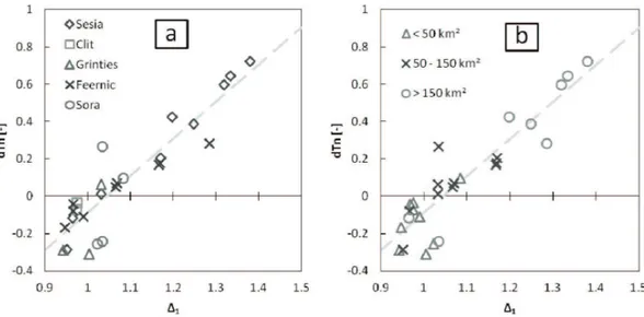
ref-erence to several flash floods in Europe. Previous work on the impact of storm velocity on hydrograph shape (Ogden et al., 1995) has shown that the effect of storm velocity is important when its magnitude become comparable to that of flood flow celerity. The significant differences between storm velocity and flood flows celerity suggests that even for these cases the values of storm velocity may be not large enough to influence the flood hydrograph shape. As a further step of the analy-sis, we examined the relationship between the statistics11
and12(Fig. 2). The analysis is carried out by dissecting the
five study catchments into a number of nested subcatchments (see Table 2), as a means to examine potential catchment scale effects on the relationship between11 and12. The
Fig. 2.Relationship between11and12:(a)for the study catchments,(b)for specific classes of catchment area.
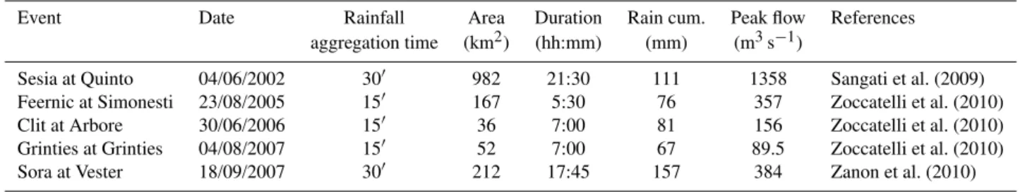
Table 1.Flood cases considered in the study.
Event Date Rainfall Area Duration Rain cum. Peak flow References aggregation time (km2) (hh:mm) (mm) (m3s−1)
Sesia at Quinto 04/06/2002 30′ 982 21:30 111 1358 Sangati et al. (2009) Feernic at Simonesti 23/08/2005 15′ 167 5:30 76 357 Zoccatelli et al. (2010) Clit at Arbore 30/06/2006 15′ 36 7:00 81 156 Zoccatelli et al. (2010) Grinties at Grinties 04/08/2007 15′ 52 7:00 67 89.5 Zoccatelli et al. (2010) Sora at Vester 18/09/2007 30′ 212 17:45 157 384 Zanon et al. (2010)
Table 2. Number and area ranges of sub-basins examined in each case study.
Event Date Number of Range of
sub-basins sub-basin areas
Sesia at Quinto 04/06/2002 9 75–982
Feernic at Simonesti 23/08/2005 9 5–167
Clit at Arbore 30/06/2006 2 12–36
Grinties at Grinties 04/08/2007 3 11–52
Sora at Vester 18/09/2007 4 32–212
catchment size ranges between 5 and 982 km2, with 9 catch-ments less than 50 km2, 10 catchments ranging between 50 and 150 km2, and 8 catchments larger than 150 km2.
Inspection of this figure shows that in 16 cases out of 27 the value of 11 falls in a narrow interval around one
(0.95< 11<1.07). In 13 cases out of these 16 cases, 12
ranges between 0.9 and 1.02, indicating that generally12is
close to one when11 is also close to one. In these cases
the first two scaled moments are virtually unchanged with respect to the spatially uniform rainfall case. However, it is
interesting to note one case of Grinties, reporting a value of 12around 0.7 in correspondence to a value of11 equal to
1.03. This is one of the few cases in which a strong rainfall concentration corresponds spatially to the geomorphologic center of mass of the catchment. When11exceeds the
up-per bound of the interval (1.07), the corresponding value of 12is lower than 0.9. There is only one case of12exceeding
1.1, indicating a case of multimodal spatial distribution of rainfall. More than half of the cases show values of11in the
range 1.05–1.4, documenting the effect of orography on the spatial rainfall distribution. Indeed, one of the elements that favour the anchoring of convective system is the orography, which play an important role in regulating of atmospheric moisture inflow to the storm and in controlling storm motion and evolution (Davolio et al., 2006). Consistently with this observation, values of11less than 0.95 are not represented
in the study floods.
As expected, all but two of the catchments with area less than 50 km2are characterized by values of11and12close
Plate 2.Precipitation analyses by using time series of precipitation intensity, coverage (for precipitation intensity>20 mm h−1),δ1(-),δ2(-)
are characterized by values of 11 larger than 1.2 and
cor-responding values of12 less than 0.8. These values
(cor-responding to subcatchments of Sesia and Feernic) imply a strong concentration of rainfall towards headwater and a cor-respondingly low dispersion around the mean values. Ac-cordingly with the analysis reported in this work, these char-acteristics should translate to a delayed and more peaky hy-drograph, with respect to the one obtained by using spatially uniform rainfall.
5 Examination of runoff model sensitivity to rainfall spatial organization by using scaled spatial moments of catchment rainfall: the case of the timing error
In this section we quantify the effect of neglecting the rain-fall spatial variability on the rainrain-fall-runoff model applica-tion. Hydrologic response from the five storm events over the 27 subcatchments analysed in Sect. 4 is examined by using a simple spatially distributed hydrologic model. The distributed model is based on availability of raster informa-tion of the landscape topography and of the soil and land use properties. In the model, the runoff rateq(x,y,t )(L T−1) at timet and location x,y is computed from the rainfall rate r(x,y,t ) (L T−1) using the Green-Ampt infiltration model with moisture redistribution (Ogden and Saghafian, 1997). The adopted formulation of the Green and Ampt model has been chosen because it provides a simple, but not simplis-tic (Barry et al., 2005) and yet physically-based description of the infiltration-excess mechanisms. A simple description of the drainage system response (Da Ros and Borga, 1997) is used to represent runoff propagation. The distributed runoff propagation procedure is based on the identification of drainage paths, and requires the characterization of hill-slope paths and channeled paths. A channelization support area (As)(L2) is used to distinguish hillslope elements from
channel elements. The model includes also a linear concep-tual reservoir for base flow modeling (Zoccatelli et al., 2010). The reservoir input is provided by the infiltrated rate com-puted based on the Green-Ampt method. The model param-eters were estimated over the catchments available for each event by means of a combination of manual and automatic calibration to minimize either the Nash-Sutcliffe efficiency index over the flood hydrographs (for the gauged catchments) or the mean square error over the flood peak and the timing data (rise, peak and recession) (for catchments where runoff data were provided from post-event surveys). Details about the application of the model to the individual events, its cali-bration and its verification are reported in the relevant papers (Sangati et al., 2009; Zoccatelli et al., 2010; Zanon et al., 2010). In general, the model simulations of the flood hy-drographs were closer to observations for the smaller basins where the linear routing approach implemented in the model provides a better description of the actual processes. In this first exploratory work we focus on the timing error (Ehret
and Zehe, 2011), i.e. the difference in the timing of the cen-troid of the hydrographs obtained by using either spatially distributed or spatially uniform rainfall, and analyse the rela-tionship between this kind of error and the11statistic. For
each subcatchment, the flash flood response was simulated by using the actual rainfall spatial variability and then by us-ing spatially uniform precipitations, hence obtainus-ing two dif-ferent hydrographs. Moreover, in order to clarify the relative roles of transport paths and of heterogeneity in the runoff generation processes, we performed numerical experiments in which the infiltration and the difference between hillslope and channel travel times are selectively “turned off”, by as-suming that the soil is impermeable and the hillslope and channel celerity have the same value.
The statistic 11 is expected to quantify the hydrograph
timing error. For storms characterised by11larger than one,
rainfall is concentrated towards the periphery of the catch-ment, with the hydrograph delayed relative to the case of a spatially uniform rainfall. The opposite is true for rainfall concentrated towards the outlet (11less than one); in these
cases the hydrograph should be anticipated relative to the case of spatially uniform rainfall. A statistic, termed “nor-malised time difference”dTn , is introduced to quantify the timing error between the two hydrographs. The normalised time differencedTnis computed by dividing the time differ-ence between the two hydrograph centroids by the response time of the catchmentE(Tc), as follows:
dTn=
E(Tq Dist)−E(Tq Unif) E(Tc)
(18) whereE(Tq−Dist)andE(Tq−Unif)are the hydrograph
cen-troids corresponding to the hydrographs generated by using spatially distributed rainfall (termed “reference hydrograph” hereinafter) and spatially uniform rainfall, respectively. A positive (negative) value ofdTnimplies a positive (negative) shift in time of the reference hydrograph with respect to the one produced by using uniform precipitation. It should be noted that Eq. (18) may written down by exploiting Eq. (10) as follows:
dTn=
E(Tq Dist)−E(Tq Unif) E(Tc)
=E(Tr)+ 11g1
v −E(Tr)− g1
v g1
v
=11−1 (19)
Equation (19) shows that the normalised timing error is re-lated in a simple way to the spatial organisation of the rain-fall fields by means of the scaled spatial moment of order one. The comparison between the two hydrographs is ex-emplified for the cases of Sesia at Quinto (982 km2) and of Grinties at Grinties (52 km2) in Fig. 3a and b, respec-tively. The storm event which triggered the Sesia flash flood was characterised by a strong concentration of rainfall to-wards the headwaters (11=1.33, 12=0.79) , which
Fig. 3. (a, b): Modelled flood hydrographs obtained by using spatially distributed and uniform precipitation, for the case of(a)Sesia at Quinto (982 km2) and(b)Grinties at Grinties (52 km2).
respect to that corresponding to the case of spatially uni-form precipitation. Correspondingly, the simulated flood peak obtained by using spatially uniform rainfall is too early (dTn=0.3) and its amplitude is too large with respect to the “reference” hydrograph. For the case of Grienties, the storm event was heavily concentrated over the catchment centroid (11=1.03,12=0.72), which has no implications in terms
of response timing (dTn=0.05) but translates to a much less peaked catchment response from spatially uniform rainfall with respect to the “reference”. Both cases show clearly the impact of neglecting the spatial distribution of rainfall in rainfall-runoff modelling even at small and moderate catch-ment sizes.
To clarify the role of runoff transport processes alone on the sensitivity of runoff model to rainfall spatial organisation, we carried out three different sets of numerical experiments. In the first case, the soil is assumed everywhere completely impervious and the hillslope celerity has the same value as the channel celerity. The rainfall-runoff model in this case is subject to the same assumptions used to derive the spatial moments statistics. Results for the relationship betweendTn and11for the various catchments are reported in Fig. 4a,
whereas Fig. 4b displays the same results for various classes of catchment size. The results show a linear relationship be-tween the two variables, as expected. The linear regression is as follows
dTn=1.001411−1.0019; r2=1 (20)
which reproduces very well Eq. (19).
In the second case, the soils are again considered impervi-ous, whereas the hillslopes and channels elements are con-sidered separately, and are characterised by the celerities identified by means of the model calibration process. Re-sults for the relationship betweendTnand11for the various
catchments are reported in Fig. 5a and b, showing again a strong linear relationship. The linear regression is as follows dTn=0.7211−0.72; r2=0.99 (21)
The introduction of the hillslope travel time leads to a de-crease of the slope of the regression line, which dede-creases from 1.0 to 0.72. This corresponds to a linear decrease of the timing error by 28 %, showing that the main effect of in-troducing the hillslope system is to decrease the influence of the rainfall spatial organisation on catchment response. It is likely that increasing the role of the hillslope residence time will further reduce the sensitivity of the hydrological model to rainfall spatial organization. The high determination co-efficient of the regression line is a remarkable finding, since the hillslope travel times were calibrated individually to each flood event. This may suggest that the relative contribution of hillslopes and channels to the average residence time is rather similar through the various events. This is not surpris-ing, given the extreme character of all the floods considered in this work.
In the third case, the model includes the actual distribu-tion of the infiltradistribu-tion parameters and different celerities are used to simulate hillslopes and channels. The relationship betweendTnand11is reported in Fig. 6a and b, whereas the
linear regression is as follows
dTn=1.9811−2.07; r2=0.83 (22)
Fig. 4. (a, b): Relationship betweendTnand11obtained by considering impervious soils and neglecting the hillslope travel time in the
hydrological model. The relationship is reported for(a)the study catchments,(b)specific classes of catchment area. The dashed line is the linear regressiondTn=1.001411−1.0019(r2=1).
Fig. 5. (a, b): Relationship betweendTnand11obtained by considering impervious soils and the hillslope travel time in the hydrological
model. The relationship is reported for(a)the study catchments,(b)specific classes of catchment area. The dashed line is the linear regressiondTn=0.7211−0.72(r2=0.99).
and b is that the slope and the intercept of the linear regres-sion are higher than those corresponding to Eq. (19). This effect is the result of the non-linearity characterizing the rain-fall to runoff transformation. Zoccatelli et al. (2010), in an investigation concerning three extreme flood events, showed that the non-linearity in the rainfall-runoff transformation leads to a magnification of the values of thedTn statistics with respect to those obtained in the impervious case. Es-sentially, this means that when rainfall is either focused on the headwaters or on the outlet, the runoff exhibits an even
stronger offset towards either the periphery of the catchment or the outlet as a result of the non-linear hydrological pro-cesses implied in the runoff generation. This effect leads to a steepening of the linear relationship betweendTnand11,
which increases from 0.72 to 1.98. Overall, the combination of the results displayed in Fig. 5a and b and Fig. 6a and b shows that the effect of the rainfall-runoff transformation on the relationship betweendTnand11are stronger, at least for
Fig. 6. (a, b): Relationship betweendTnand11obtained by considering infiltration and the hillslope travel time in the hydrological model.
The relationship is reported for(a)the study catchments,(b)specific classes of catchment area. The dashed line is the linear regression
dTn=1.9811−2.07(r2=0.83).
that the method based on the spatial moments provides use-ful information on the potential impact of the rainfall spatial organisation on the features of the ensuing flood hydrograph, in spite of the assumptions used for its derivation.
6 Discussion and conclusion
In this paper, we proposed a new set of spatial rainfall statis-tics which assess the dependence of the catchment flood re-sponse on the space-time interaction between rainfall and the spatial organization of catchment flow pathways. Named “spatial moments of catchment rainfall”, these statistics de-scribe the spatial rainfall organisation in terms of concen-tration and dispersion statistics as a function of the distance measured along the flow path coordinate. The introduction of the spatial moments of catchment rainfall permits deriva-tion of the concept of catchment scale storm velocity, which quantifies the up or down-basin rainfall movement as filtered by the catchment morphological properties relative to the storm kinematics. The work shows how the first two spatial moments afford quantification of the impact of rainfall spa-tial organization on two fundamental properties of the flood hydrograph: timing (surrogated by the runoff mean time) and amplitude (surrogated by the runoff time variance). The first spatial moment provides a measure of the scaled distance from the geographical centroid of the rainfall spatial pattern to the catchment centroid. The second spatial moment pro-vides a scaled measure of the additional variance in runoff time that is caused by the spatial rainfall organization, rela-tive to the case of spatially uniform rainfall.
The analysis reported here suggests that the proposed rain-fall statistics are effective in (i) describing the degree of spa-tial organisation which is important for runoff modelling and (ii) quantifying the relevance of rainfall spatial variability on flood modeling, with specific reference to the timing error. This is an essential aspect of this work, since our outcome clearly shows that catchment response is sensitive to spatial heterogeneity of rainfall even at small catchment sizes. The timing error introduced by neglecting the rainfall spatial vari-ability ranges between−30 % to 72 % of the corresponding catchment response time. It should be borne in mind that the floods considered in this work are very intense flash floods characterised by strong rainfall gradients.
We believe that the main strength of the method lies in a better understanding of the linkages between the charac-teristics of the rainfall spatial patterns with the shape and magnitude of the catchment flood response. This provides an indicator at catchment scale that integrates morphology and rainfall space-time distribution, and that can be used to compare influence of rainfall distribution across basins and scales. This is a fundamental aspect, since it enables evalu-ating the accuracy with which rainfall space and time distri-bution need to be observed for a given type of storm event and for a given catchment. For example, this may provide new statistics and criteria both for defining the optimality of raingauge network design in areas where flash floods are ex-pected and for evaluating the accuracy of radar rainfall esti-mation algorithms and attendant space-time resolution.
and quantifying hydrological similarity across a wide range of rainfall events and catchments, within the broader frame-work of comparative hydrology. For instance, the method can be used to identify the features of catchment morphology which attenuates (or magnify) the effects of rainfall space-time organization. With the use of the spatial moments, the interaction of rainfall forcing and catchment characteristics can be described not only in terms of mean areal rainfall, but also by considering the features of rainfall spatial concentra-tion and the storm velocity. For example, this may help to reveal the effect of orography not only on the precipitation accumulation at the catchment scale, but also on the space-time organization of the rainfall patterns.
Further research should also focus on the concept of the catchment scale storm velocity. The introduction of this con-cept permits assessment of its significance for actual flood cases and analyses of the space and time rainfall sampling schemes which are required for its adequate estimation for various catchment scales and configurations. There is also a need to extend the formulation of the spatial moments of catchment rainfall to incorporate the hillslope transit time as a way to conceptualise the impact of the hillslope system on the catchment’s filtering properties.
Finally, the rainfall statistics introduced in this paper could be used as an input to a new generation of semi-distributed hydrological models able to use the full range of statistics, and not only the mean areal rainfall, for flood modeling and forecasting. This will permit extending the capabilities of this class of hydrological models to rainfall events character-ized by significant rainfall variability.
Appendix A
In this Appendix we show how Eqs. (10), (13) and (15) may be derived from V2010. For this, we start from Eqs. (19), (23) and (25) in V2010.
A1 Derivation of Eq. (10)
Equation (19) in V2010 (Eq. V19 hereinafter) provides the average time to route the rainfall excess from the geograph-ical centroid of the rainfall spatial pattern to the catchment outlet. Using the same notation used in the current work, Eq. (V19) is written down as follows:
E(Tc)= g1
v +
Covx,y[d(x,y),rt(x,y)] vP0
(A1) where Covx,y[]is the spatial covariance.
Equation A1 is developed as follows to derive Eq. (10): E(Tc)=gv1+Covx,y[d(x,y),rtvP (x,y)]
0 =
=g1
v +
R
A
d(x,y)rt(x,y)dA AvP0 −
g1
v = P1
P0v=
11g1
v
(A2)
A2 Derivation of Eq. (13)
Equation (23) in V2010 (Eq. V23 hereinafter) provides the variance of the time to route the rainfall excess to the catch-ment outlet. Using the same notation used in the current work, Eq. (V23) is written down as follows:
Var(Tc)=
g2−g12
v2 +
Covx,y[d(x,y)2,rt(x,y)]
v2P
0 +
−Covx,y[d(x,y),rtvP (x,y)]
0
h
2g1
v +
Covx,y[d(x,y),rt(x,y)] vP0
i (A3)
Equation (A3) is developed as follows to derive Eq. (13):
Var(Tc)=
g2−g12
v2 +
R
A
d(x,y)2rt(x,y)dA Av2P
0 − g2 v2 − P1
P0v−
g1
v
P1
P0v+
g1 v = P2
P0−
P12 P02
1
v2 =
12(g2−g12)
v2 .
A3 Derivation of Eq. (15)
Equation (25) in V2010 (Eq. V25 hereinafter) provides the covariance between the rainfall time and the routing time. Using the same notation used in the current work, Eq. (V25) is written down as follows:
Cov(Tr,Tc)=
CovtT ,Covx,y[d(x,y),r(x,y,t )] vP0
−Covt[T ,p0(t )] P0
Covx,y[d(x,y),rt(x,y)] vP0
(A4) Equation (A4) is developed as follows to derive Eq. (15): Cov(Tr,Tc)=g1Covt[T ,δv1(t )w(t )]−g1Covt[T ,w(t )v ]
−Covt[T ,w(t )] v
Covx,y[d(x,y),rt(x,y)] P0 =
g1Covt[T ,δv1(t )w(t )]−Covt[T ,w(t )v ](g1+11g1−g1)=
g1
Covt[T ,δ1(t )w(t )] v
| {z }
term1
−Covt[T ,w(t )] v
| {z }
term2 11 .
Acknowledgements. The work presented in this paper has been carried out as part of the European Union FP6 Project HYDRATE (Project no. 037024) under the thematic priority, Sustainable Development, Global Change and Ecosystems and by the Research Project GEO-RISKS (University of Padova, STPD08RWBY).
References
Andr´eassian, V., Perrin, C., Michel, C., Usart-Sanchez, I., and Lavabre, J.: Impact of imperfect rainfall knowledge on the effi-ciency and the parameters of watershed models, J. Hydrol., 250, 206–223, 2001.
Barry, D., Parlange, J.-Y., Li, L., Jeng, D.-S., and Crapper, M.: Green-Ampt approximations, Adv. Water. Res., 28, 1003–1009, doi:10.1016/j.advwatres.2005.03.010, 2005.
Bell, V. A. and Moore, R. J.: The sensitivity of catchment runoff models to rainfall data at different spatial scales, Hydrol. Earth Syst. Sci., 4, 653–667, doi:10.5194/hess-4-653-2000, 2000. Berne, A., Delrieu, G., Creutin, J. D., and Obled, C.: Temporal and
spatial resolution of rainfall measurements required for urban hy-drology, J. Hydrol., 299, 166–179, 2004.
Bl¨oschl, G.: Hydrologic synthesis: across processes, places, and scales, Water Resour. Res., 42, W03S02, doi:10.1029/2005WR004319, 2006.
Bl¨oschl, G. and Sivapalan, M.: Scale issues in hydrological mod-elling: a review, Hydrol. Process., 9, 251–290, 1995.
Borga, M., Boscolo, P., Zanon, F., and Sangati, M.: Hydrometeoro-logical analysis of the August 29, 2003 flash flood in the eastern Italian Alps, J. Hydrometeorol., 8, 1049–1067, 2007.
Borga, M., Gaume, E., Creutin ,J. D., and Marchi, L.: Surveying flash flood response: gauging the ungauged extremes, Hydrol. Process., 22, 3883–3885, doi:10.1002/hyp.7111, 2008.
Borga, M., Anagnostou, E. N., Bl¨oschl, G., and Creutin, J. D.: Flash Floods: observations and analysis of hydrometeorological con-trols, J. Hydrol., 394, 1–3, doi:10.1016/j.jhydrol.2010.07.048, 2010.
Bouilloud, L., Delrieu, G., Boudevillain, B., Kirstetter, P.E.: Radar rainfall estimation in the context of post-event analysis of flash-flood events, J. Hydrol., 394, 17–27, doi:10.1016/j.jhydrol.2010.02.035, 2010.
D’Odorico, P. and Rigon, R.: Hillslope and channel contribu-tions to the hydrologic response. Water Resour. Res., 39, 1113, doi:10.1029/2002WR001708, 2003.
Da Ros, D. and Borga, M.: Use of digital elevation model data for the derivation of the geomorphologic instantaneous unit hydro-graph, Hydrol. Process,, 11, 13–33, 1997.
Davolio, S., Buzzi, A., and Malguzzi, P.: Orographic influence on deep convention: case study and sensitivity experiments, Meteo-rol. Z., 15 , 215–223, 2006.
De Lima, J. L. and Singh, V. P.: The influence of the pattern of moving rainstorms on overland flow, Adv. Water. Res, 25, 817– 828, 2002.
Ehret, U. and Zehe, E.: Series distance – an intuitive metric to quan-tify hydrograph similarity in terms of occurrence, amplitude and timing of hydrological events, Hydrol. Earth Syst. Sci., 15, 877– 896, doi:10.5194/hess-15-877-2011, 2011.
Fabry, F.: On the determination of scale ranges for precipitation fields, J. Geophys. Res., 101, 12819–12826, 1996.
Goltz, M. and Roberts, P. .: Using the Method of Moments to Analyze Three-Dimensional Diffusion-Limited Solute Transport From Temporal and Spatial Perspectives, Water Resour. Res., 23, 1575–1585, 1987.
Gourley, J., Hong, J., Flamig, Z. L., Wang, J., Vergara, H., and Anagnostou, E. N.: Hydrologic Evaluation of Rainfall Esti-mates from Radar, Satellite, Gauge, and Combinations on Ft. Cobb Basin, Oklahoma, J. Hydrometeorol., 12, 5, 973–988,
doi:10.1175/2011JHM1287.1, 2011.
Krajewski, W. F. and Smith, J. A.: Radar hydrology-rainfall estima-tion, Adv. Water. Res., 25, 1387–1394, 2002.
Maksimov, V. A.: Computing runoff produced by a heavy rainstorm with a moving center, Soviet Hydrology, 5, 510–513, 1964. Marani, M.: Non-power-law-scale properties of rainfall
in space and time, Water Resour. Res., 41, W08413, doi:10.1029/2004WR003822, 2005.
Marchi, L., Borga, M., Preciso, E., and Gaume, E.: Character-isation of selected extreme flash floods in Europe and impli-cations for flood risk management, J. Hydrol, 394, 118–133, doi:10.1016/j.jhydrol.2010.07.017, 2010.
McDonnell, J. J. and Woods, R.: On the need for catchment classi?cation. J. Hydrol., 299, 2–3, doi:10.1016/j.jhydrol.2004.09.003, 2004.
Morin, E., Goodrich, D. C., Maddox, R. A., Gao, X. G., Gupta, H. V., and Sorooshian, S.: Spatial patterns in thunderstorm rainfall events and their coupling with water-shed hydrological response, Adv. Water Res., 29, 843–860, doi:10.1016/j.advwatres.2005.07.014, 2006.
Moulin, L., Gaume, E., and Obled, C.: Uncertainties on mean areal precipitation: assessment and impact on streamflow simulations, Hydrol. Earth Syst. Sci., 13, 99–114, doi:10.5194/hess-13-99-2009, 2009.
Naden, P. S.: Spatial variability in flood estimation for large catch-ments: the exploitation of channel network structure, Hydrol. Sci. J., 37, 53–71, 1992.
Nic´otina, L., Alessi Celegon, E., Rinaldo, A., and Marani, M.: On the impact of rainfall patterns on the hydrologic response, Water Resour. Res., 44, W12401, doi:10.1029/2007WR006654, 2008. Niemczynowicz, J.: Investigation of the influence of rainfall
move-ment on runoff hydrograph: Part I. Simulation of conceptual catchment, Nordic Hydrology, 15, 57–70, 1984.
Obled, C., Wendling, J., and Beven, K.: Sensitivity of hydrological models to spatial rainfall patterns: An evaluation using observed data, J. Hydrol, 159, 305–333, 1994.
Ogden, F. L. and Julien, P., Y.: Runoff model sensitivity to radar rainfall resolution, J. Hydrol, 158, 1–18, 1994.
Ogden, F. L. and Saghafian, B.: Green and Ampt infiltration with redistribution, J. Irrig. Drain. Eng., 123, 386–393, 1997. Ogden, F. L., Richardson, J. R., and Julien, P. Y.: Similarity in
catchment response: 2. Moving rainstorms, Water Resour. Res., 31, 1543–1547, 1995.
Pellarin, T., Delrieu, G., Saulnier, G. M., Andrieu, H., Vignal, B., Creutin, J. D.: Hydrologic visibility of weather radar systems operating in mountainous regions: Case study for the Ardeche Catchment (France), J. Hydrometeorol., 3, 539–555, 2002. Rinaldo, A., Botter, G., Bertuzzo, E., Uccelli, A., Settin, T., and
Marani, M.: Transport at basin scales: 1. Theoretical frame-work, Hydrol. Earth Syst. Sci., 10, 19–29, doi:10.5194/hess-10-19-2006, 2006.
Robinson, J., Sivapalan, M., and Snell, J.: On the relative roles of hillslope processes, channel routing, and network geomorphol-ogy in the hydrologic response of natural catchments., Water Re-sour. Res., 31 , 3089–3101, 1995.
Rodriguez-Iturbe, I. and Valdes, J. B.: The geomorphologic struc-ture of hydrologic response, Water Resour. Res., 15, 1409–1420, 1979.
On spacetime scaling of cumulated rainfall fields, Water Resour. Res., 34, 3461–3469, 1998.
Saco, P. and Kumar, P.: Kinematic dispersion in stream networks – 1. Coupling hydraulic and network geometry, Water Resour. Res., 38, 1244, doi:10.1029/2001WR000695, 2002.
Sangati, M., Borga, M., Rabuffetti, D., and Bechini, R.: Influence of rainfall and soil properties spatial aggregation on extreme flash flood response modelling: an evaluation based on the Sesia river basin, North Western Italy, Adv. Water. Res, 32, 1090–1106, 2009.
Saulnier, G. and Le Lay, M.: Sensitivity of flash-flood simulations on the volume, the intensity, and the localization of rainfall in the Cevennes-Vivarais region (France), Water Resour. Res., 45, W10425, doi:10.1029/2008WR006906, 2009.
Singh, V. P.: Effect of the direction of storm movement on planar flow, Hydrol. Process., 12, 147–170, 1998.
Skøien, J. O. and Bl¨oschl, G.: Catchments as space-time filters – a joint spatio-temporal geostatistical analysis of runoff and precip-itation, Hydrol. Earth Syst. Sci., 10, 645–662, doi:10.5194/hess-10-645-2006, 2006.
Skøien, J. O., Bl¨oschl, G., and Western, A.: Characteristic space scales and timescales in hydrology, Water Resour. Res., 39, 1304. doi:10.1029/2002WR001736, 2003.
Smith, J. A., Baeck, M. L., Morrison, J. E., Sturdevant-Rees, P. L., Turner-Gillespie, D. F., and Bates, P. D.: The regional hydrology of extreme floods in an urbanizing drainage basin, J. Hydrome-teorol., 3, 267–282, 2002.
Smith, J. A., Baeck, M. L., Meierdiercks, K. L., Nelson, P. A., Miller, A. J., and Holland, E. J.: Field studies of the storm event hydrologic response in an urbanizing watershed, Water Resour. Res., 41, W10413, doi:10.1029/2004WR003712, 2005. Smith, M. B., Seo, D.-J., Koren, V. I., Reed, S., Zhang, Z., Duan,
Q.-Y., Cong, S., and Moreda, F.: The distributed model inter-comparison project (DMIP): motivation and experiment design, J. Hydrol., 298, 4–26, 2004a.
Smith, M., Koren, V., Zhang, Z., Reed, S., Pan, J., and Moreda, F.: Runoff response to spatial variability in precipitation: an analysis of observed data, J. Hydrol., 298, 267–286, 2004b.
Surkan, A. J.: Simulation of storm velocity effects of flow from distributed channel network, Water Resour. Res., 10, 1149–1160, 1974.
Syed, K., Goodrich, D., Myers, D., and Sorooshian, S.: Spatial characteristics of thunderstorm rainfall fields and their relation to runoff, J. Hydrol., 271, 1–21, 2003.
Viglione, A., Chirico, G. B., Woods, R., and Bl¨oschl, G.: Generalised synthesis of space-time variability in flood re-sponse: An analytical framework, J. Hydrol., 394, 198–212, doi:10.1016/j.jhydrol.2010.05.047, 2010a.
Viglione, A., Chirico, G. B., Komma, J., Woods, R., Borga, M., and Bl¨oschl, G.: Quantifying space-time dy-namics of flood event types, J. Hydrol., 394, 213–229, doi:10.1016/j.jhydrol.2010.05.041, 2010b.
Woods, R.: A search for fundamental scales in runoff generation: combined field and modelling approach, Ph.D. Thesis, Depart-ment of EnvironDepart-mental Engineering, University of Western Aus-tralia, Nedlans, Western AusAus-tralia, 1997.
Woods, R. A. and Sivapalan, M.: A synthesis of space-time vari-ability in storm response: Rainfall, runoff generation and rout-ing, Water Resour. Res. , 35, 2469–2485, 1999.
Zhang, Y., Smith, J. A., and Baeck, M. L.: The hydrology and hy-drometeorology of extreme floods in the Great Plains of eastern Nebraska, Adv. Water Resour., 24, 1037–1050, 2001.
Zanon, F., Borga, M., Zoccatelli, D., Marchi, L., Gaume, E., Bon-nifait, L., and Delrieu, G.: Hydrological analysis of a flash flood across a climatic and geologic gradient: the September 18, 2007 event in Western Slovenia, J. Hydrol., 394, 182–197, doi:10.1016/j.jhydrol.2010.08.020, 2010.
Zoccatelli, D. and Wuletawu, R.: Role of hillslope and channel res-idence time on runoff model sensitivity to spatial rainfall organi-zation, Report of University of Padova, 74 pp., 2010.