Computing the Dimensions of Boxes
from Single Perspective Images
Leandro A. F. Fernandes
1, Manuel M. Oliveira
1, Roberto da Silva
1& Gustavo J. Crespo
21Universidade Federal do Rio Grande do Sul
Instituto de Inform´atica - PPGC - CP 15064 91501-970 - Porto Alegre - RS - BRAZIL {laffernandes, oliveira, rdasilva}@inf.ufrgs.br
2Stony Brook University
Department of Computer Science - 11794 New York - NY - USA
{gus crespo}@yahoo.com
Abstract
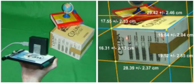
This paper describes an accurate method for com-puting the dimensions of boxes directly from perspective projection images acquired by conventional cameras. The approach is based on projective geometry and computes the box dimensions using data extracted from the box si-lhouette and from the projection of two parallel laser be-ams on one of the imaged faces of the box. In order to identify the box silhouette, we have developed a statis-tical model for homogeneous-background-color removal that works with a moving camera, and an efficient voting scheme for the Hough transform that allows the identifi-cation of almost collinear groups of pixels. We demons-trate the effectiveness of the proposed approach by auto-matically computing the dimensions of real boxes using a scanner prototype that implements the algorithms and methods described in the paper. We also present a discus-sion of the performed measurements, and an error propa-gation analysis that allows the method to estimate, from each single video frame, the uncertainty associated to all measurements made over that frame, in real-time.
Keywords: Computing dimensions of boxes,
image-based metrology, extraction of geometric information from scenes, uncertainty analysis, real time.
Figure 1. Scanner prototype: (left) Its operation. (right) Camera’s view from another position showing the recovered dimensions and
uncertainty computed in real time.
1. I
NTRODUCTIONThe ability to measure the dimensions of three-dimensional objects directly from images has many prac-tical applications including quality control, surveillance, analysis of forensic records, storage management and cost estimation. Unfortunately, unless some information rela-ting distances measured in image space to distances me-asured in 3D is available, the problem of making mea-surements directly on images is not well defined. This results from the inherent ambiguity of perspective projec-tion caused by the loss of depth informaprojec-tion.
even when the target box is partially occluded by other objects in the scene (Figure 1). We eliminate the inherent ambiguity associated with perspective images by projec-ting two parallel laser beams, apart from each other by a known distance, onto one of the visible faces of the box. We demonstrate this technique by building a scanner pro-totype for computing box dimensions and using it to com-pute the dimensions of boxes in real time (Figure 1). This can be an invaluable tool for companies that manipulate boxes on their day-by-day operations, such as couriers, airlines and warehouses.
The paper presents a revised and significantly exten-ded version of the work originally described in [9]. The new materials in this extended version include: (i) the use of variable-size elliptical Gaussian kernels in the Hough transform voting procedure (Section 5). The use of such kernels makes the transform more robust to discretization errors and allows the proper detection of support silhou-ette lines of boxes with bent edges; (ii) the determination of the plane spanned by the laser beams using a calibra-tion procedure (Subseccalibra-tion 3.2.1). The use of calibrated data removed the only assumption in the original deriva-tion [9] of the equaderiva-tions shown in Secderiva-tion 3 and improved the accuracy of the method; (iii) the statistical analysis of the results (Section 7.1) was significantly enhanced con-sidering a larger number of real boxes and new graphs that improve the interpretation of these results. Such an analysis shows that the proposed approach is both accu-rate and precise; and (iv) a modeling of the error propaga-tion along all steps of the algorithm that allows our system to estimate the uncertainty in the computed measurements in real time (Section 7.2).
The main contributions of this paper include:
• An algorithm for computing the dimensions of bo-xes in a completely automatic way in real-time (Sec-tion 3);
• An algorithm for extracting box silhouettes in the presence of partial occlusion of the box edges (Sec-tion 3.1);
• A statistical model of homogeneous background co-lor for use with a moving camera under different lighting conditions (Section 4);
• An efficient voting scheme for identifying nearly collinear line segments with a Hough transform (Section 5);
• A derivation of how to estimate the error associated with the computed dimensions from a single image in real time (Section 7.2).
2. R
ELATEDW
ORKMany optical devices have been created for making measurements in the real world. Those based on active techniques project some kind of energy onto the surfa-ces of the target objects and analyze the reflected energy. Examples of active techniques include optical triangula-tion [1] and laser range finding [22] to capture the shapes of objects at proper scale [17], and ultrasound to measure distances [10]. In contrast, passive techniques rely only on the use of cameras for extracting the three-dimensional structure of a scene and are primarily based on the use of stereo [18]. In order to achieve metric reconstruction [13], both optical triangulation and stereo-based systems re-quire careful calibration. For optical triangulation, several images of the target object with a superimposed moving pattern are usually required for accurate reconstruction.
Labeling schemes for trihedral junctions [4, 15] have been used to estimate the spatial orientation of polyhe-dral objects from images. These techniques tend to be computationally expensive when too many junctions are identified. Additional information from the shading of the objects can be used to improve the process. Silhouettes have been used in computer vision and computer graphics for object shape extraction [16, 21]. These techniques re-quire precise camera calibration and use silhouettes obtai-ned from multiple images to define a set of cones whose intersections approximate the shapes of the objects.
Criminisi et al. [5] presented a technique for making 3D affine measurements from a single perspective image. They show how to compute distances between planes pa-rallel to a reference one. In case of some distance from a scene element to the reference plane is known, it is possible to compute the distances between scene points and the reference plane. If such a distance is not known, the computed dimensions are correct up to a scaling fac-tor. The technique requires user interaction and cannot be used for computing dimensions automatically. Pho-togrammetrists have also made measurements based on single images [23], but these techniques also require user intervention.
In a work closely related to ours, Lu [20] described a method for finding the dimensions of boxes from single gray-scale images. In order to simplify the task, Lu as-sumes that the images are acquired using parallel ortho-graphic projection and that three faces of the box are visi-ble simultaneously. The computed dimensions are appro-ximately correct up to a scaling factor. Also, special care is required to distinguish the actual box edges from lines in the box texture, causing the method not to perform in real time.
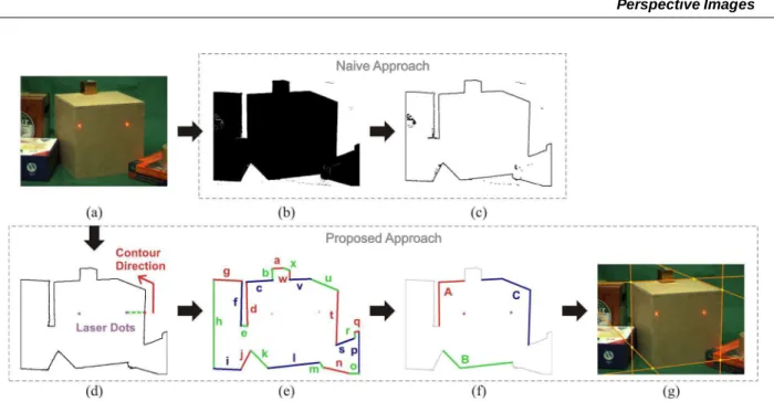
Figure 2. Identifying the target box silhouette. Naive approach: (b) Background segmentation, followed by (c) High-pass filter (note the spurious “edge” pixels). Proposed approach: (d) Contouring of the foreground region, (e) Contour segmentation, (f) Grouping candidate segments for the
target silhouette, and (g) Recovery of supporting lines for silhouette edges and vertices.
textures, can be used when only two faces of the box are visible, even when the edges of the target box are partially occluded by other objects in the scene.
3. C
OMPUTINGB
OXD
IMENSIONS We model boxes as parallelepipeds although real bo-xes can present many imperfections (e.g., bent edges and corners, asymmetries, etc.). The dimensions of a paralle-lepiped can be computed from the 3D coordinates of four of its non-coplanar vertices. Conceptually, the 3D coor-dinates of the vertices of a box can be obtained by inter-secting rays, defined by the camera’s center and the pro-jections of the box vertices on the camera’s image plane, with the planes containing the actual faces of the box in 3D. Thus, before one can compute the dimensions of a gi-ven box (Section 3.3), its necessary to find the projections of the vertices on the image (Section 3.1), and then find the equations of the planes containing the box faces in 3D (Section 3.2).In the following derivations, we assume that the ori-gin of the image coordinate system is at the center of the image, with theX-axis growing to the right and theY -axis growing down, and assume that the imaged boxes have three visible faces. The case involving only two visi-ble faces is similar. Also, we assume that the images used for computing the dimensions were obtained through li-near projection (i.e., using a pinhole camera). Although images obtained with real cameras contain some amount of radial and tangential distortions, we compensate such distortions in real time with the use of simple warping
procedures [13].
The number of visible faces of the box can be ob-tained by checking if the projection of some of the ed-ges that share the same direction in 3D is (almost) pa-rallel in 2D. In this case, two faces of the box are vi-sible; otherwise, three faces are visible simultaneously. Although this approach has proven to produce good re-sults for well-constructed boxes, most real boxes present some distorted edges, which breaks the parallelism sumption. Thus, in practice, it is more effective to as-sume that three box faces are visible. Since the system is capable of computing the dimensions of boxes at30Hz, we can afford to discard frames if the silhouettes recove-red from the acquirecove-red images do not satisfy the imposed requirements. In this case, the perception of the user is similar to that of a barcode scanner user: if no answer is coming out, just slightly change the scanner’s orientation relatively to the target object in order to get it.
3.1. FINDING THE PROJECTIONS OF THE VERTI -CES
requi-red and will be discussed in detail in Section 4.
However, as shown in Figure 2 (a, b and c), a naive ap-proach that just models the background and applies sim-ple image processing operations, like background remo-val and high-pass filtering, does not properly identify the silhouette pixels of the target box (selected by the user by pointing the laser beams onto one of its faces). This is because the scene may contain other objects, whose si-lhouettes possibly overlap with the one of the target box. Also, the occurrence of some misclassified pixels (see Fi-gure 2, c) may lead to the detection of spurious edges. Thus, a suitable method was developed to deal with these problems. The steps of our algorithm are shown in Figu-res 2 (a, d, e, f and g).
In our approach, the target box silhouette is obtained starting from one of the laser dots, finding a silhouette pixel and using a contour-following procedure [12]. The seed silhouette pixel for the contour-following is found stepping from the laser dot within the target foreground region and checking whether the current pixel matches the background model. In order to be a valid silhouette, both laser dots need to fall inside of the contouring re-gion. Notice this procedure produces a much cleaner set of border pixels (Figure 2, d) compared to results shown in Figure 2 (c). But the resulting silhouette may include overlapping objects, and one still needs to identify which border pixels belong to the target box. To facilitate the handling of the border pixels, the contour is subdivided into its most perceptually significant straight line seg-ments [19] (Figure 2, e). Then, the segseg-ments resulting from the clipping of a foreground object against the limits of the frame (e.g., segmentsh,oandpin Figure 2, e) are discarded. Since a box silhouette defines a convex poly-gon, the remaining segments whose two endpoints are not visible by both laser dots can also be discarded. This test is performed using a 2D BSP-tree [11]. In the example of Figure 2, only segmentsc,d,k,l,t,uandvpass this test. Still, there is no guarantee that all the remaining seg-ments belong to the target box silhouette. In order to res-trict the amount of possible combinations, the remaining chains of segments defining convex fragments are grou-ped (e.g., groupsA,BandCin Figure 2, f). We then try to find the largest combination of groups into valid por-tions of the silhouette. In order to be considered a valid combination, the groups must satisfy the following vali-dation rules: (i) they must characterize a convex polygon; (ii) the silhouette must have six edges (the silhouette of a parallelepiped with at least two visible faces); (iii) the laser dots must be on the same box face; and (iv) the com-puted lengths for pairs of parallel edges in 3D must be approximately the same. In the case of more than one combination of groups pass the validation tests, the sys-tem discards this ambiguous data and starts processing a new frame (our system is capable of processing frames at
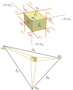
Figure 3. Vanishing points (ωi) and vanishing lines (λi).ej,vj,m0,
andfiare the supporting lines for silhouette edges, the silhouette
vertices, the inner vertex and the faces of the box, respectively.
the rate of about29fps).
Once the box silhouette is known, the projections of the six vertices are obtained intersecting pairs of adja-cent supporting lines for the silhouette edges (Figure 2, g). Section 5 discusses how to obtain those supporting lines.
3.2. COMPUTING THEPLANEEQUATIONS
The set of all parallel lines in 3D sharing the same direction intersect at a point at infinite whose image un-der perspective projection is called a vanishing pointω. The line defined by all vanishing points from all sets of parallel lines on a planeΠis called the vanishing lineλ
ofΠ(Figure 3). The normal vector toΠin a given ca-mera’s coordinate system can be obtained multiplying the transpose of the camera’s intrinsic-parameter matrix by the coefficients of λ[13]. Since the resulting vector is not necessarily a unit vector, it needs to be normalized. Equations (1) and (2) and Figure 3 show the relationship among the vanishing pointsωi, vanishing linesλiand the
supporting linesej for the edges that coincide with the
imaged silhouette of a parallelepiped with three visible faces. The supporting lines are ordered clockwise.
ωi=ei×ei+3 (1)
λi=ωi×ω(i+1)mod3 (2)
where0 ≤i ≤2,0 ≤j ≤5,λi = (aλi, bλi, cλi)
T and
Πiis then given by
NΠi=
RKTλ i
kRKTλ ik
(3)
whereNΠi = (AΠi, BΠi, CΠi).Kis the matrix that mo-dels the intrinsic camera parameters [13] andR is a re-flection matrix (Equation 4) used to make theY-axis of the image coordinate system grows in the up direction.
K=
αx γ ox
0 αy oy
0 0 1
, R=
1 0 0
0 −1 0
0 0 1
(4)
In Equation (4),αx = f /sxandαy =f /sy, where f is the focal length, andsxandsyare the dimensions of
the pixel in centimeters. γ,oxandoy represent the skew
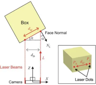
and the coordinates of the principal point, respectively. Once we have NΠi, findingDΠi, the fourth coeffi-cient of the plane equation, is equivalent to solving the projective ambiguity and will require the introduction of one more constraint. Thus, consider the situation depic-ted in 2D in Figure 4 (left), where two laser beams, pa-rallel to each other, are projected onto one of the faces of the box. Let the 3D coordinates of the laser dots de-fined with respect to the camera coordinate system be
P0 = (XP0, YP0, ZP0)
T and P
1 = (XP1, YP1, ZP1) T,
respectively (Figure 4, right). SinceP0andP1are on the
same planeΠ, one can write
AΠXP0+BΠYP0+CΠZP0=AΠXP1+BΠYP1+CΠZP1
(5) Using the linear projection model and given
pi= (xpi, ypi,1)
T, the homogeneous coordinates of
the pixel associated with the projection of pointPi, one
can reprojectpion the planeZ = 1(in 3D) using
p′ i= (xp′
i, yp′i,1)
T =RK−1p
i (6)
and express the 3D coordinates of the laser dots on the face of the box as
XPi =xp′iZPi , YPi =yp′iZPi and ZPi (7)
Substituting the expression for XP0, YP0, XP1 and YP1(Equation 7) in Equation (5) and solving forZP0, we
obtain
ZP0 =kZP1 (8)
where
k=AΠxp′1+BΠyp′1+CΠ AΠxp′
0+BΠyp′0+CΠ
(9)
Now, letdlbanddldbe the distances, in 3D, between
the two parallel laser beams and between the two laser dots projected onto one of the faces of the box, respecti-vely (Figure 4). Section 6 discusses how to find the laser dots on the image.dldcan be directly computed fromNΠ,
Figure 4. Top view of a scene. Two laser beams apart in 3D bydlb
project onto one box face at pointsP0andP1, whose distance in 3D is
dld.αis the angle between−LandNL.
the normal vector of the face onto which the dots project, and the known distancedlb:
dld= dlb
cos(α) =
dlb
−(NL·L)
(10)
whereαis the angle betweenNL, the normalized
projec-tion ofNΠonto the plane defined by the two laser beams,
andLis the vector representing the laser beam direction. For now, we will assume that the laser plane is parallel to the cameraXZplane andL= (0,0,1)T. Therefore,N
L
is obtained by dropping theY coordinate ofNΠand
nor-malizing the resulting vector.dldcan also be expressed as
the Euclidean distance between the two laser dots in 3D:
d2ld= (XP1−XP0) 2+(Y
P1−YP0) 2+(Z
P1−ZP0) 2 (11)
Substituting Equations (7), (8) and (10) into (11) and sol-ving forZP1, one gets
ZP1= s
d2 ld
ak2−2bk+c (12)
wherea= (xp′ 0)
2+ (y p′
0)
2+ 1,b=x p′
0xp′1+yp′0yp′1+ 1
andc= (xp′ 1)
2+ (y p′
1)
2+ 1. GivenZ
P1, the 3D
coordi-nates ofP1can be computed as
P1= (XP1, YP1, ZP1) T = (x
p′
1ZP1, yp′1ZP1, ZP1) T
(13) The projective ambiguity can be finally removed by computing theDΠcoefficient for the plane equation of
the face containing the two dots:
3.2.1. Estimating the Laser Plane: In practice, it is difficult to guarantee that the plane defined by the laser beams is parallel to the camera’sXZplane, and that the
Lvector is aligned with the cameraZ-axis. In our scan-ner prototype, we noticed that although the laser beams are parallel to each other, the plane they define (Πlb) is
not parallel to the camera’sXZplane. Therefore, it is ne-cessary to take into account the angle between these two planes before computingNLand thendld(Equation 10).
The orientation ofΠlband the direction of theL
vec-tor were estimated projecting the laser beams on a planar checkerboard calibration pattern, placed at varying dis-tances from the scanner. By collecting the coordinates of a set of 3D points (corresponding to these projections) along the laser lines, we estimated bothΠlb’s orientation
andL’s direction with respect to the camera’s coordinate system.
3.3. COMPUTING THEBOXDIMENSIONS
Having computed the plane equation of a face of the box, one can recover the 3D coordinates of vertices of that face. For each such vertexvon the image, we computev′
using Equation (6). We then compute its corresponding
ZV coordinate by substituting Equation (7) into the plane
equation for the face. GivenZV, bothXV andYV
coor-dinates are computed using Equation (7). Since all visible faces of the box share some vertices with each other, the D coefficients for the other faces of the box can also be obtained, allowing the recovery of the 3D coordinates of all vertices on the box silhouette, from which the dimen-sions are computed.
Although not required for computing the dimensions of the box, the 3D coordinates of the inner vertexm0
(Fi-gure 3, top) can also be computed. Its 2D coordinates are obtained as the intersection among three lines. Each such line is defined by a vanishing point and the silhou-ette vertex falling in between the two box edges used to compute that vanishing point. This situation is illustra-ted in Figure 3. Since it is unlikely that these three lines will intersect exactly at one point, we approximate this in-tersection using least-squares. Given the inner vertex 2D coordinates, its corresponding 3D coordinates are com-puted using the same algorithm used to compute the 3D coordinates of the other vertices.
4. A M
ODEL FORB
ACKGROUNDP
I-XELS
In order to obtain the box silhouette, we need to clas-sify the pixels as either background or foreground pixels. One of the most popular techniques for object segmenta-tion is chroma keying [24]. Unfortunately, standard ch-roma keying techniques do not produce satisfactory
re-Figure 5. Chromaticity axis rotated to align to a horizontal axis. The curve is a polynomial fit to the chromaticity distortion threshold for
each slice (the small rectangles).
sults for our application. Shading variations in the back-ground and shadows cast by the boxes usually lend to mis-classification of background pixels. Horprasert et al. [14] describe a statistical method that computes a per-pixel model of the background from a set of static background images. While this technique is fast and produces very good segmentation results for scenes acquired from a sta-tic camera, it is not appropriate for use with moving ca-meras. Also it requires a complete new calibration when the lighting conditions change too much. To avoid pro-blems from lighting changes, a threshold solution based on hue component of the HSV color space might seem to be a good solution. However, such an approach tends to misclassify foreground pixels whose colors are close to the background color.
In order to support a moving camera, we have deve-loped an approach that proved to be robust, lending to very satisfactory results. It works under different lighting conditions by computing a statistical model of the back-ground, which contains a single hue. Such a model is defined by a chromaticity axis that represents the mean expected shade of the background under various lighting conditions and a polynomial curve describing a variable threshold along the chromaticity axis.
The algorithm takes as input a set ofnimagesIiof the
background acquired under different lighting conditions. In the first step, we computeE, the average color of all pixels in all imagesIi, and the eigenvalues and
eigenvec-tors associated with the colors of those pixels.Eand the eigenvector associated with the highest eigenvalue define an axis in the RGB color space (the chromaticity axis). The chromaticity distortiondof a given colorCis com-puted as the distance fromCto the chromaticity axis.
After discarding the pixels whose projections on the chromaticity axis have at least one saturated channel (they lend to misclassification of bright foreground pixels), we subdivide the chromaticity axis intomslices (Figure 5). For each slice, we compute d¯j andσd¯j, the mean and
the standard deviation, respectively, for the chromaticity distortion of the pixels in the slice. Then, we com-pute a thresholddT j for the maximum acceptable
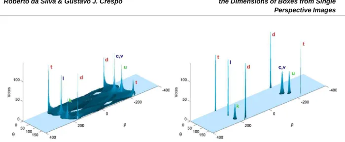
Figure 6. Hough Transform parameter space obtained with the conventional (left) and the new voting scheme (right) applied to the segments shown in Figure 2 (f). The peaks represent the supporting lines for silhouette edges.
99%asdT j= ¯dj+ 2.33σd¯j.
Finally, the coefficients of a polynomial that models the chromaticity-distortion thresholds are computed by fitting a curve through thedT values at the centers of the
slices (Figure 5). Intuitively, such a polynomial describes a variable threshold for the different shades of the back-ground color. Once the coefficients have been computed, thedT values are discarded and the tests are performed
against the model. Figure 5 illustrates the case of a color
Cbeing tested against the background color model.C′is
the projection ofCon the chromaticity axis. In this exam-ple, as the distance betweenCand the chromaticity axis is bigger than the threshold defined by the polynomial,C
will be classified as foreground.
Changing the background color only requires obtai-ning samples of the new background and computing the new values for the chromaticity axis and the coefficients of the polynomial. It is possible that the box texture may contain some pixels whose chromaticity distortions are smaller than the threshold defined by the polynomial for a given background color shade. In this case, the classi-fication process would incorrectly indicate the presence of background pixels inside the box region. However, the silhouette detection approach described in Section 3.1 can handle groups of misclassified foreground pixels and, in practice, no problems have been noticed as a result of possible such misclassification. According to our experi-ments,100slices and a polynomial of degree 3 produce very satisfactory results.
5. I
DENTIFYINGA
LMOSTC
OLLINEARS
EGMENTSTo compute the image coordinates of the box vertices, first we need to obtain the supporting lines for the silhou-ette edges. We do this using a Hough transform proce-dure [7]. However, the conventional voting process and
the detection of the most significant lines is computatio-nally intensive and turned out to be a bottleneck to our system. To reduce the amount of computation, an alterna-tive to the conventional voting process was developed.
As seen in Section 3.1, silhouette pixels are organized into perceptually most significant straight-line segments. The new voting scheme consists in casting votes directly for these segments, instead of for individual pixels as it is traditionally done [7]. Thus, for each segment, the(ρ, θ)
parameters of its supporting line are computed from the average position of the set of pixels defining the segment and from the 2D eigenvectors of that pixel distribution. The eigenvector with the smaller eigenvalue is the nor-mal to the line, soρcan be computed as the dot product between this eigenvector and the average pixel. θis the angle between theX-axis of the image and the secondary eigenvector. The use of eigenvectors makes the process robust, allowing it to handle lines with arbitrary orientati-ons in a corientati-onsistent way.
For each segment, we distribute its votes in the para-meter space using a Gaussian elliptical kernel (Figure 6, right), whose central position is defined by the(ρ, θ) para-meters of the line fit to its set of pixels. The Gaussian ker-nel spread the votes over a region of the parameters space around(ρ, θ), according to the quality of the fit. Notice however, that different segments have different numbers of pixels, as well as have different degrees of dispersion around their corresponding best-fitting lines. The smaller the dispersion, the more concentrated these votes should be in the parameter space. We estimate the quality of the line fit by computing the variances and covariance of the
a first order uncertainty propagation analysis [25] to com-pute the variances and covariance ofρandθfrom the va-riances and covava-riances of the slope-intercept parameters. Once one has computed the variances and covariance as-sociated withρandθ, the votes are cast using a bi-variated Gaussian distribution [26]. The use of a Gaussian kernel distributes the votes around a neighborhood, allowing the identification of approximately collinear segments. This is a very important and unique feature of our approach that allows our system to better handle discretization er-rors and boxes with slightly bent edges. A detailed ex-planation about the proposed voting process can be found in [8].
Using the new approach, the voting process and the peak detection are significantly improved because the amount of cells that receive votes is substantially redu-ced. Figure 6 shows the parameter space after the traditi-onal (left) and the new (right) voting processes have been applied to the segments shown in Figure 2 (f). Using the conventional (i.e., per-pixel) voting scheme [7],376,884
votes are distributed over 228,255 cells. In contrast, the new approach only casts6,382votes distributed over
5,020cells, which represents1.7%of the number of votes and2.2%of the number of cells used in the conventional approach. As a result, the produced voting map is very clean (Figure 6, right), reducing ambiguities and impro-ving the identification of the most important lines. The extra cost involved in computing the covariance matrices associated with a few segments and by the use of Gaus-sian elliptical kernels to cast votes is more than compen-sated by the huge saving achieved.
Special care must be taken when theθ parameter is close to0◦or to180◦. In this situation, the voting process
continues in the diagonally opposing quadrant, at the−ρ
position (see Figure 6, peaksdandt). For the examples shown in the paper, the parameter space was discretized using360angular steps in the rangeθ = [0◦,180◦)and
1,600ρvalues in the range[−400,400].
6. F
INDING THEL
ASERD
OTSThe ability to find the proper positions of the laser dots in the image can be affected by several factors such as the camera’s shutter speed, the box materials and textu-res, and ambient illumination. Although we are using a red laser (650nm class II), we cannot rely simply on the red channel of the image to identify the positions of the dots. Such a procedure would not distinguish between the laser dot and red texture elements on the box. Since the pixels corresponding to the laser dots present very high lu-minance, we identify them by thresholding the luminance image. However, just simple thresholding may not work for boxes containing white regions, which tend to have
large areas with saturated pixels. We solved this problem by setting the camera’s shutter speed so that the laser dots are the only elements in the image with high luminance.
Since the image of a laser spot is composed by seve-ral pixels, we approximate the actual position of the dot by the centroid of its pixels. According to our experi-ments, a variation of one pixel in the estimated center of the laser spot produces a variation of a few millimeters in the computed dimensions. These numbers were obtai-ned assuming a camera standing about two meters from the box. After computing the position of the inner ver-tex (Section 3.3), the face that contains the laser dots is identified.
The system may fail to properly detect the laser dots if they project on some black region or if the surface exhi-bits specular peaks. This, however, can be avoided by aiming the beams on other portions of the box. Due to the construction of the scanner prototype and to some epipo-lar constraints [13], one only needs to search for the laser dots inside a small window in the image. Although a sin-gle laser beam could be used to break the projective am-biguity, the use of two beams introduces additional cons-traints that make silhouette identification more robust.
7. R
ESULTSWe have built a prototype of a scanner for compu-ting box dimensions and implemented the techniques des-cribed in the paper using C++. The system was tested on several real boxes. For a typical scene, such as the one shown in Figure 2, it can process video and com-pute box dimensions at about29 fps. For comparison, the frame rate drops to 10 fps if the traditional pixel-based Hough-transform voting scheme (Figure 6, left) is used. Such numbers illustrate the effectiveness of the pro-posed voting solution. These measurements were made on a2.8GHz PC with1.0GB of memory. A video se-quence illustrating the use of our scanner can be found at http://www.inf.ufrgs.br/˜laffernandes/boxdimensions.
Figure 1 (left) shows the scanner prototype whose hardware is comprised of a firewire color camera (Point Grey Research DragonFly with640×480pixels), a16
mm lens (Computar M1614, with manual focus, no iris and30.9degrees horizontal field of view) and two laser pointers. The camera is mounted on a plastic box and the laser pointers were aligned and glued to the sides of this box. In such an assembly, the laser beams are15.8cm apart. For our experiments, we acquired pictures of boxes from distances varying from1.7to3.0 meters to the ca-mera. The background was created using a piece of green cloth and its statistical model was computed from a set of
(a) (b)
(c) (d)
(e) (f)
(g) (h)
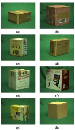
Figure 7. Examples of real boxes used for testing.
challenging: (e), (f) and (g) are very bright; (f) and (g) have a reflective plastic finishing; and box (b) is mostly covered with red texture. The dimensions of these boxes vary from13.8to48.2cm. The intrinsic parameters of the camera (Equation 4) were estimated using a calibrations procedure [2].
The geometry of the box is somewhat different from a parallelepiped due to imperfections introduced during construction and handling. For instance, bent edges, dif-ferent sizes for two parallel edges of the same face, lack of parallelism between opposing faces, and warped corners are not unlikely to be found in practice. Such inconsisten-cies lend to errors in the orientation of the silhouette ed-ges, which are cascaded into the computation of the box dimensions.
In order to estimate the inherent inaccuracies of the proposed algorithm, we performed measurements on a wooden box (Figure 7, h) that was carefully constructed to avoid these imperfections. We have also implemented a simulator that performs the same computations on images of synthetic boxes (exact parallelepipeds) generated using
computer graphics techniques. Using images generated by the simulator, our system can recover the dimensions of the box with an average relative error of0.58%. Next, we analyze some of the results obtained on real boxes.
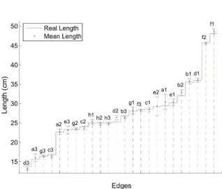
7.1. STATISTICALANALYSIS ONREALBOXES In order to evaluate the effectiveness of the proposed approach, we carried out a few statistical experiments. First, we selected several real boxes (Figure 7) and ma-nually measured the dimensions of all their edges with a ruler. Each edge was measured twice, once per shared face of the edge. The eight measurements of each box dimensions were averaged to produce a single value per dimension. All measurements were made in centimeters. We then used our system to collect a total of30 measure-ments of each dimension of the same box. For each col-lected sample, we projected the laser beams on different parts of the box. We used this data to compute the mean, standard deviation and confidence intervals for each of the computed dimensions. The confidence intervals were
computed asCI = hx¯−tγ√σ
n,x¯+tγ σ √ n
i
, wherex¯is the mean,σis the standard deviation,nis the size of sam-ple andtγ is at−Student variable withn−1degrees of
freedom, such that the probability of a measurexbelongs toCIisγ. The tightest theCI, the more precise are the computed values.
Figure 8 shows the computed confidence intervals withγ= 99.5%. Note that the values of the actual di-mensions (the red line) fall inside most these confidence intervals, indicating accurate measurements. Boxes (f), (g) and especially the wooden box (h) are the ones with tightest confidence intervals. Those are well constructed boxes. Wider confidence intervals were obtained for bo-xes with bent faces and edges, like bobo-xes (a) and (e). The only box whose actual dimensions do not fall inside the confidence interval is box (d). This box has a cardboard lid that changes the box silhouette, shifting the computed mean values away from the true ones.
Another estimate of the error can be expressed as the relative errorǫ=|x−xv|/xv, wherexis the computed
dimension andxvis the value of the actual dimension.
Fi-gure 9 shows a histogram of the relative errors in the me-asurements obtained with our scanner prototype for the boxes shown in Figure 7. The higher relative errors were computed for boxes (a), (d) and (e) (the ones exhibiting imperfections) and is in accordance with the experiment summarized in Figure 8. Considering all measurements, the mean relative error for all real boxes is3.75%, indica-ting very good accuracy.
7.2. ERRORPROPAGATION
fol-Figure 8. Confidence intervals computed from measurements of the edges of the boxes shown in Figure 7. The boxes edges are sorted by
length.
lowing error propagation model [25]:
Λw=∇fΛϑ∇fT (15)
whereΛwis the covariance matrix that models the errors
inw;∇fis the Jacobian matrix for the functionf(ϑ)that computes each term ofwfrom theninput variables; and
Λϑ is the covariance matrix that models the errors of the
input variables. The model assumes a Gaussian distribu-tion of the errors around the mean values estimated by
f(ϑ)and allows the computation of confidence intervals for the length of each visible edge using a single input image.
To apply this error propagation model, one needs to estimate the error associated to each input variable. In the proposed method, the input variables are:
• hi = (ρi, θi)T,0 ≤ i ≤ 5: the coefficients of the
normal equation of the supporting lines for the si-lhouette edges (12 variables);
• pj = xpj, ypj
T
,0≤j≤1: the image coordinates of the laser dots (4 variables);
• dlb: the distance between the laser beams (1
varia-ble);
• K: the camera’s intrinsic-parameters matrix (5 vari-ables);
• L = (XL, YL, ZL)T: the laser beam direction (3
variables).
So,Λϑ is a25×25covariance matrix, comprised by
the variances and covariances of all input variables:
Λϑ=diag(Λh0, . . . ,Λh5,Λp0,Λp1,Λddb,ΛK,ΛL) (16)
Figure 9. Histogram of the relative errors in the computed dimensions for the edges of the boxes in Figure 7.
Given these variables, the Jacobian of the function that computes the length of the target box edges can be ob-tained as shown in Equation 17. The partial derivatives in∇f are calculated using the chain rule over the set of equations presented in Section 3.
∇f = ∂w ∂ρ0
∂w ∂θ0 . . .
∂w ∂XL
∂w ∂YL
∂w ∂ZL
(17)
The error propagation model expressed by Equati-ons 15, 16 and 17 allows our system to estimate the un-certainty associated with the measurement of each edge of the box in real time. This information can be used to discard unreliable measurements, which may result if the box is relatively far from the camera, or if one of the box edges approaches a direction almost perpendicular to the cameras image plane.
Special care must be taken when choosing the dis-tance between the laser beams. The uncertainty in the computed dimensions increases as the lasers distance de-creases, because the relative error tends to increase as the distance becomes smaller. However, the distance between the laser beams constrains the minimal accepted size for a box, since both laser dots must fall inside the same face. So, for a given application, one should consider a trade-off between the minimal box size and the accepted uncer-tainty in the measurements.
8. C
ONCLUSIONS ANDF
UTUREW
ORK We have presented a completely automatic approach for computing the dimensions of boxes from single pers-pective projection images in real time. The approach uses information extracted from the silhouette of the target box and removes the projective ambiguity with the use of two parallel laser beams. We demonstrated the effectiveness of the proposed techniques by building a prototype of a scanner and using it to compute the dimensions of seve-ral real boxes even when the edges of the target box are partially occluded by other objects.approxima-tely collinear segments using a Hough transform, and a statistical model for background removal that works with a moving camera and under different lighting conditions. We validated the proposed approach performing a statisti-cal analysis over measurements obtained with our scanner prototype from real boxes. In addition, we presented an analytical derivation of uncertainty propagated along the entire computation chain that allows real-time estimation of the error in the computed measurements. The statistics and experimental validation have shown that the proposed approach is accurate and precise.
Our algorithm for computing box dimensions can also be used by applications requiring heterogeneous back-grounds. For that, background detection can be perfor-med using a technique like the one described in [14]. In this case, the camera should remain static while the boxes are moved on some conveyor belt.
We believe that these ideas may lead to optimizations on several procedures that are currently based on manual measurements of box dimensions. We are currently ex-ploring ways of using arbitrary backgrounds with a mo-ving camera.
Acknowledgments
This work was partially sponsored by CNPq - Bra-sil (Processo No 477344/2003-8), Petrobras (Processo 502009/2003-9), and Microsoft Brazil.
References
[1] P. Besl. Active Optical Range Imaging Sensors. Ad-vances in Machine Vision, pages 1–63. Springer-Verlag, New York, NY, USA, 1988.
[2] J. Y. Bouguet. Camera calibration toolbox for ma-tlab. http://www.vision.caltech.edu/ bouguetj/ ca-lib doc, Jan. 2005.
[3] J. Canny. A computational approach to edge detec-tion. IEEE Transactions on Pattern Analysis and Machine Intelligence, 8(6):679–698, Nov. 1986.
[4] M. B. Clowes. On seeing things. Artificial Intelli-gence, 2:79–116, 1971.
[5] A. Criminisi, I. Reid, and A. Zisserman. Single view metrology. In Proceedings of the 7th IEEE Interna-tional Conference on Computer Vision (ICCV-99), volume 1, pages 434–441, Kerkyra, Greece, Sept. 1999. IEEE Computer Society.
[6] N. R. Draper and H. Smith. Applied Regression Analysis. John Wiley & Sons, New York, 1966.
[7] R. O. Duda and P. E. Hart. Use of the Hough transformation to detect lines and curves in pictu-res. Communications of the ACM, 15(1):11–15, Jan. 1972.
[8] L. A. F. Fernandes. Um m´etodo projetivo para c´alculo de dimens˜oes de caixas em tempo real. Mas-ter’s thesis, Universidade Federal do Rio Grande do Sul, Porto Alegre, RS, Brazil, Jan. 2006. (in Portu-guese).
[9] L. A. F. Fernandes, M. M. Oliveira, R. da Silva, and G. Crespo. Computing box dimensions from single perspective images in real time. In Procee-dings of XVIII Brazilian Symposium on Computer Graphics and Image Processing (SIBGRAPI 2005), pages 155–162, Natal, RN, Brazil, Oct. 2005. IEEE Computer Society.
[10] F. Figueroa and A. Mahajan. A robust method to determine the coordinates of a wave source for 3-D position sensing. ASME Journal of Dynamic Systems, Measurements and Control, 116:505–511, Sept. 1994.
[11] H. Fuchs, Z. M. Kedem, and B. F. Naylor. On visible surface generation by a priori tree structures. In Pro-ceedings of the 7th Annual Conference on Computer Graphics and Interactive Techniques (SIGGRAPH-80), pages 124–133, New Orleans, Louisiana, 1980. ACM Press.
[12] J. Gauch. KUIM, image processing system. http://www.ittc.ku.edu/˜jgauch/research, Jan. 2003.
[13] R. I. Hartley and A. Zisserman. Multiple View Ge-ometry in Computer Vision. Cambridge University Press, Cambridge, UK, 2000.
[14] T. Horprasert, D. Harwood, and L. S. Davis. A statistical approach for real-time robust background subtraction and shadow detection. In Proceedings of the 7th IEEE ICCV-99, FRAME-RATE Workshop, Kerkyra, Greece, Sept. 1999. IEEE Computer Soci-ety.
[15] D. A. Huffman. Impossible objects as nonsense sentences. In Machine Intelligence, volume 6, pa-ges 295–324. Edinburg University Press, Edinburg, 1971.
[17] M. Levoy, K. Pulli, B. Curless, S. Rusinkiewicz, D. Koller, L. Pereira, M. Ginzton, S. Anderson, J. Davis, J. Ginsberg, J. Shade, and D. Fulk. The digital Michelangelo project: 3D scanning of large statues. In Proceedings of the 27th Annual Confe-rence on Computer Graphics and Interactive Tech-niques (SIGGRAPH-00), pages 131–144, New Or-leans, Louisiana, Jul. 2000. ACM Press.
[18] H. C. Longuet-Higgins. A computer algorithm for reconstructing a scene from two projections. Nature, 293:133–135, Sept. 1981.
[19] D. G. Lowe. Three-dimensional object recognition from single two-dimensional images. Artificial In-telligence, 31:355–395, Mar. 1987.
[20] K. Lu. Box dimension finding from a single gray-scale image. Master’s thesis, SUNY Stony Brook, New York, 2000.
[21] W. Matusik, C. Buehler, R. Raskar, S. J. Gortler, and L. McMillan. Image-based visual hulls. In Proce-edings of the 27th Annual Conference on Computer Graphics and Interactive Techniques (SIGGRAPH-00), pages 369–374, New Orleans, Louisiana, Jul. 2000. ACM Press.
[22] L. Nyland, D. McAllister, V. Popescu, C. McCue, A. Lastra, P. Rademacher, M. Oliveira, G. Bishop, G. Meenakshisundaram, M. Cutts, and H. Fu-chs. The impact of dense range data on computer graphics. In Proceedings of Multi-View Modeling and Analysis Workshop (MVIEW99), pages 3–10, Fort Collins, CO, Jun. 1999. IEEE Computer Soci-ety.
[23] J. W. H. Tangelder, P. Ermes, G. Vosselman, and F. A. van den Heuvel. Cad-based photogramme-try for reverse engineering of industrial installations. Computer-Aided Civil and Infrastructure Enginee-ring, 18:264–274, Jul. 2003.
[24] P. Vlahos. Composite color photography. U.S. Pa-tent 3.158.477, 1964.
[25] J. H. Vuolo. Fundamentos da Teoria de Erros. Ed-gard Blcher, S˜ao Paulo, SP, Brazil, 1992. (in Portu-guese).