A Macroeconomic Model of Credit Risk in
Uruguay
Gabriel Illanes
*
, Alejandro Pena
†
, Andrés Sosa
‡
Contents: 1. Introduction; 2. Credit risk models; 3. Applications by sectors in the Uruguayan economy; 4. Conclusions.
Keywords: Credit Risk, Default, Structural Models, Central Banking, Test Stress. JEL Code: E58.
In this paper we evaluate credit risk of the economy as a whole, aiming at the study of the financial stability. This analysis uses as proxy the credit granted by the banking system. We use a non-linear parametric model based on Merton’s structural framework for the analysis of the risk associated to a loan portfolio. In this model, default occurs when the return of an economic agent falls under certain threshold which depends on different macroeconomic variables. We use this model to assess the credit risk module in stress tests for the local banking system. We also estimate the “elasticities” of credit categories correspondig to corporate credit and consumer credit, both in national currency and american dollars. We obtain the parameters for the model using maximum likelihood, where the likelihood function contains a random latent factor which is assumed to follow a normal distribution.
Neste artigo avaliamos o risco de crédito para toda a economia, almejando o estudo da estabilidade financeira. Esta análise usa como proxy o crédito distribuído pelo sis-tema bancário. Usamos um modelo paramétrico não-linear, baseado no framework estrutural de Merton, para análise do risco associado a cada portfólio de emprésti-mos. Neste modelo, o default ocorre quando o retorno de um agente econômico cai abaixo de um certo ponto de corte que depende de diferentes variáveis macroeconô-micas. Usamos este modelo para acessar o módulo de risco de crédito em testes de estresse para o sistema bancário local. Também estimamos as “elasticidades” das categorias de crédito correspondentes ao crédito corporativo e crédito pessoal, tanto em moeda local como em dólares americanos. Obtemos os parâmetros para o modelo maximizando uma função verossimilhança que contém um fator aleatório latente com distribuição normal.
*Universidad de la República, Facultad de Ciencias, Centro de Matemática. Iguá 4225, Esq. Mataojo, Montevideo, Uruguay.
CP 11400. Email:[email protected]
†Banco Central del Uruguay, Superintendencia de Servicios Financieros, Departamento Riesgos Financieros. Diagonal Fabini 777,
Montevideo, Uruguay. CP 11100. Email:[email protected]
‡Universidad de la República, Facultad de Ciencias, Centro de Matemática. Iguá 4225, Esq. Mataojo, Montevideo, Uruguay.
1. INTRODUCTION
There are two types of basic strategies to model credit risk, and from each one of them a group of models is obtained. The first group of models estimates risk factors at an individual level. These models have been developed mostly by commercial banks, in order to develop credit policies. These models can evaluate the risk of every borrower; however, procyclicality in credit evaluation is a problem, which consist in being too optimist during boom times, and too pessimistic during low economy cycles. Some examples of this kind of models are IRB model (Internal Ratings-Based Approach), advocated by Basel II as the simplest internal model for credit risk evaluation and the assess of the required capital by that risk.
The credit risk model we use belongs to the second group, in which the aggregate credit risk for the whole economy is estimated, and then used to evaluate financial stability. The default rate of the economy is an input variable of stress tests, for which it is important to have a way to estimate it.
In particular, one of our objectives is to present a one-factor credit risk model for a loan portfo-lio. We want a model able to estimate the proportion of defaulted loans in economy as a response to the evolution of different macroeconomic variables. There exists a wide range of empirical work and applications for this kind of models, for example Céspedes & Martín (2002), Cipollini & Missaglia (2005), Hamerle, Leibig, & Scheule (2004), Lucas & Klaassen (2003), Rosch (2003) and Rosch (2005).
In section 2 we describe the economic risk model for a loan portfolio, compute the default proba-bility without conditioning to the random latent factor, compute the likelihood function to be optimized, and explain how to select the macroeconomic variables most related to every credit category. In sec-tion 3 we describe the available data to fit the models, and then we present and discuss the obtained results for every model. In section 4 we discuss the results and conclude.
2. CREDIT RISK MODELS
The objective of credit risk models is to quantify possible losses in case of counterparty default. The default risk for the economy as a whole is estimated in order to study the stability of he financial system.
This kind of models have been studied in depth for several decades. There exists an extensive literature based on default probabilities for individual borrowers and for the economy as a whole, or for a given commercial bank of the system. For the former case, dependencies between macroeconomic variables and credit risk are established. For the latter case, one possible variant for the model is to use a model for panel data to estimate the parameters at a global level, taking into account the information of each one of the banks.
2.1. Credit risk models used by the central banks
Credit risk models used by Central Banks are used for stress tests and have the objective of assessing the financial stability of the bank system. Therefore, they belong to the group of models that evaluate the aggregate credit risk. Most of credit risk models are either structural models or reduced models. However, there exist another kind of model that aims to keep the best features of both structural and reduced models; they are called hybrid models.
Structural models are based on Merton (1974), in which the debtor’s capability to meet obligations is studied, computing the probability of debtor’s assets fall under certain thershold. These models are widely known in the financial markets, and they are used by important financial firms. The hypothesis is that investors have all market information, and they have full knowledge about assets and debts values of all firms. The structural models include among others the models presented in Geske (1977) and J.P. Morgan & Co. (1997).
probability of meeting obligations have the same structure as a discount factor. The reduced models are include in Duffie & Singleton (1997) and Jarrow & Turnbull (1995) where the advantages of this approach of credit risk are introduced.
2.2. Review of credit models applied to financial systems
The most traditional approach for the study of credit risk consists in obtaining an empirical relation-ship between a dependent variable representing the credit quality of a loan portfolio, and a set of mar-coeconomic variables to be selected. This methodology was used by Central Banks in United Kingdom, Germany, Belgium, Finland and Czech Republic (Jakubík, 2007).
The Bank of England (Bunn, Cunningham, & Drehmann, 2005), used this model to estimate the default rate of loans granted to non-financial companies, loans granted to individuals for house purchase secured by a mortage, and in credit card portfolios. This default rates are estimated from variables such as gross domestic product, real interest rate, unemployment rate, companies indebtedness level and other macroeconomic indicators.
In the case of the Bank of Finland (Virolainen, 2004), uses an empirical model based on a logistic re-gression that aims to explain default rate of different sectors of the economy, also using macroeconomic variables.
Linear approximations can be reasonable when shock is small, but when shocks are large it might be necessary to introduce non-linear factors. Based on this concept, the Bank of Canada (Coletti et al., 2008), studied the relationship between a logistic transformation of the default rate of different sectors of the economy and two macroeconomic variables—gross domestic product and interest rate— transformed by polynomial functions.
The Bank of Japan (2007), used a probit transformation of the probability of a rating transitions in which the independent variables are the gross domestic product growth and the ratio of interest bearing liability to cash flow.
The Bank of Spain (Jiménez & Mencía, 2007), used a probit transformation of the default rate and the independent variables are change in the real gross domestic product growth, interest rate, term spread, six sectoral variables and two latent factors (unobserved common factors).
In Latin America, there are few references available of application of this methods. In Caicedo Ce-rezo, Bielsa, & Casanovas Ramón (2011), credit risk is quantified using Merton’s model for companies in the Colombian market between 2005 and 2007.
In the case of Uruguay, no publications about default probability estimation using structural mod-els were found. For that reason, this paper can become the first reference in the application of structural models and credit risk assessment for Uruguayan economy as a whole.
2.3. Mathematical model
The model assumes a homogeneous portfolio of companies in the economy. The standardized log-return of companyi in timetsatisfies the equation
R(ti)= √ρFt+√1−ρUt(i), (1) whereF is the logarithm of the returns in the economy, independent of companyi(systematic factor of
economy) and it is modeled using a standard normal distribution;U(i) is the specific return of company
i, which is also modeled using a standard normal distribution; and factorρ represents the sensitivity
of the return to the non-observable factor of the economy. We will also assume that variablesF andU
We say that companyi defaults when its returnRt(i)falls below certain thresholdT. If we define the random variableY as a binary random variable taking value1if companyidefaults and0otherwise, we obtain the following equation for default probability for companyi on timetis
pt(i)=P(Yt(i)=1
)
=P(Rt(i)<T
)
.
Default thresholdT can be set as a constant, or it can be modeled using macroeconomic variables related to the economy. We choose the latter, modeling the default threshold as a linear combination of
N macroeconomic variables,
pt(i)=P
( Yt(i)=1
)
=P
(
√ρF
t+√1−ρUt(i)<β0+
N
∑
j=1 βjxjt
)
=Φ
( β0+
N
∑
j=1 βjxjt
)
,
whereΦis the standard normal distribution function.
The probability of default, conditioned to the non observable factor ft is given by
p(i)(ft)=P*
,U
(i)
t <
β0+∑Nj=1βjxjt−√ρ ft
√
1−ρ +-=Φ*,
β0+∑Nj=1βjxjt−√ρ ft
√
1−ρ +-, (2)
the formula which can also be written as
Φ−1( p(i)(ft)
)
=
β0+∑Nj=1βjxjt
√1
−ρ −
√ρ √1
−ρft
. (3)
As companies can be regarded as homogeneous, if the number of companies grows, the default rate DRt converges to the conditional probability of default. This means that we can estimate the
default rate of the portfolio by the individual probability of default.
We assume that the number of companies in default at time t conditioned to the latent factor
dt(ft) follows a binomial distribution, where the parameters are the conditional probability of default
p(i)(f
t)and the total number of companiesnt.
The non-conditional probability of default can be obtained integrating over the non-observable random factor
P(
Dt =dt)=
∫ +∞
−∞
Cnt
dt(p(ft))
dt
(1−p(ft))nt−dtϕ(ft)dt, (4)
whereϕis the standard normal density function.
The model assumes portfolios of all agents are homogeneous. This hypothesis is commonly used in literature, such as Bluhm & Overbeck (2003), Jakubík (2005) and Vasicek (1987). However, this hy-pothesis is not always met in practice; this is mostly due to different sizes of portfolios, and different recovery rates for portfolios of similar sizes. There exists a large body of literature in panel data econo-metrics pointing out the various consequences for inferences of neglecting heterogeneity. This problem has been addressed using several different approaches, for example, using quadratic factors in a two-factor model to capture the effects of different sizes of portfolios (Barone-Adesi, Gagliardini, & Urga, 2000), adding random variables representing different recovery rates (Molins & Vives, 2016), and the application of models using Markov Chain Monte Carlo (Luo & Shevchenko, 2013).
maximum likelihood. The logarithm of the likelihood function for the random vector (Dt)t∈1. . .T is
l(β¯,ρ)=
t=T
∑
t=1
log(P(
Dt=dt)
)
=
t=T
∑
t=1
log
∫ +∞
−∞
Cnt
dt (
p(ft)
)dt(
1−p(ft)
)nt−dt ϕ(ft)dt
=
t=T
∑
t=1
log
∫ +∞
−∞
Cnt
dt Φ* ,
β0+∑Nj=1βjxjt−√ρ ft
√
1−ρ +
- dt
1−Φ*
,
β0+∑Nj=1βjxjt−√ρ ft
√
1−ρ +
-
nt−dt
ϕ(ft)dt
. (5)
Now we have to find parameters β¯and ρ such that functionl presents an absolute maximum for those values. In our case, we have the problem of approximating integral (5), because its primitive function can not be computed. This problem is studied in depth in Jakubík (2005). Here, we will use the Gaussian quadrature method.
The estimated coefficientsβ¯can not be interpreted as elasticities of the impacts of macroeconomic variables on the credit risk, due to different scales of the variables and non-linearity of the model.
2.4. Adjustment of the model
There are several macroeconomic variables related to credit risk which can be used to fit the model. We would like those variables to meet the hypotheses of the model; this is, normality of Ft in (1) and independence of conditional probabilities of default (2).
Taking this into consideration, we will select a subset of macroeconomic variables for which those hypotheses are met. We observe that, if the hypotheses of the model are met, and if dt
nt is a good
ap-proximation ofp(i)(f
t), then the residuals of a multiple linear regression with dntt as dependent variable and the (possibly lagged) macroeconomic variables as independent variables should be independent and normally distributed.
All the macroeconomic variables that could predict the probabilitiesp(i) should be considered,
making the regressions of vectorp(i)(f
t) against the different choices of subgroups of such variables with the purpose of choosing the subgroups that adjusts best to the tests. It is convenient to verify not only that the signs of the coefficientsβi be coherent with the economic intuition, but also that the coefficients are statistically significant.
Therefore, we will consider all macroeconomic variables related top(i), and we will regressp(i)(f
t) against all possible subsets of the macroeconomic variables. We will select the subset of variables that best fits the hypothesis test for normality of the residuals. We will also verify that the regression coeffi-cients βi are significant, and that the sign of βi do not contradict economic intuition for the macroe-conomic variable i. Independence of the residuals can also be tested and used as a subset selection
criterion, possibly adding lagged values of the dependent variable dt
nt as independent variables (this
will not work if lagged values of dt
nt are too important as explanatory variables).
3. APPLICATIONS BY SECTORS IN THE URUGUAYAN ECONOMY
for consumer credit in dollars and corporate credit in national currency are also shown. For this purpose, we will use a data set consisting of monthly observations of different macroeconomic variables.
3.1. Data set
We will fit all models using a data set consisting of monthly observations, from December 2001 until May 2013 (138 observations in total). For every economy sector, the dependent variable is the observed proportion of defaulted loans in the private banking system corresponding to that sector. In order to weight properly the importance of people or companies in default, and also in order to respect homo-geneity hypothesis as much as we can, we will assume all loans to grant the same amount of money. It must be noted that, as the selected likelihood function (5) is not linear, results will slightly depend on the selected amount of money for an individual loan.
We remark that, during the observation time, the largest values of default rate of the banking system are obtained in 2003, due to a deep economic crisis in Uruguay. After that period, we observe a decreasing trend in the default rate due to economic growth.
We fitted for the proportion of defaulted loans for four sectors: corporate credit and consumer credit, for both national currency and American dollars. The available macroeconomic variables we considered to fit the models are:
• Country Risk of Uruguay (CR). EMBIG computed by JP Morgan. Source: Bloomberg. • Inflation Rate (IR). Source: National Institute of Statistics, Uruguay (INE).
• Lending Rate for Corporations in American Dollars (LRCorD). Source: Central Bank of Uruguay. • Lending Rate for Corporations in Uruguayan Pesos (LRCorP). Source: Central Bank of Uruguay. • Lending Rate for Consumers in American Dollars (LRConD). Source: Central Bank of Uruguay. • Lending Rate for Consumers in Uruguayan Pesos (LRConP). Source: Central Bank of Uruguay. • Monthly activity indicator based on Gross Domestic Product (GDP). Quarterly observations adapted
linearly to monthly observations.
• Nominal Exchange Rate (NER). Source: Central Bank of Uruguay. • Real Exchange Rate (RER). Source: Central Bank of Uruguay.
• Real Wage Index (RW). Source: National Institute of Statistics, Uruguay (INE). • Six-month Libor Rate (LR). Source: Bloomberg.
• Unemployment Rate (UR). Unemployment rate for the whole country, considering towns and cities over 5,000 inhabitants.
Macroeconomic variables exhibit great volatility in 2003 due to financial crisis. As well, large variance in some of the variables is also observed during 2008–2009. This is due to world financial crisis because Uruguay is a small open economy, not significant in international markets and vulnerable to different external impacts.
There are some international macroeconomic variables that are not taken into account directly, that might affect credit default risk. Some of them are commodity prices, foreign interest rates and measures of external volatility. However, we can capture some of their variability via the considered macroeconomic variables.
Regarding the international interest rates, we only consider six-month Libor Rate. However, we consider different Uruguayan interest rates which usually depend on the evolution of the Libor rate. Six-month Libor rate is not selected for any of the fitted models, but this does not mean that it does not affect credit risk.
We are not considering variables that measure the volatility of international markets, such as VIX (Chicago Board Options Exchange Market Volatility Index). However, VIX variable is highly correlated with Uruguayan Country Risk, therefore, we consider the volatility of international markets in an indirect way.
3.2. Consumer Credit in National Currency
3.2.1. Fitting the model
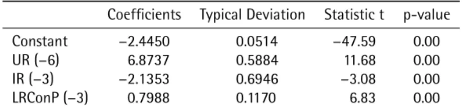
Following the variable selection criterion established in section 2.4, we found that a suitable subset of macroeconomic variables for consumer credit in national currency is (6-months lagged) Unemployment Rate, (3-months lagged) lending rate for consumers in Uruguayan pesos, and (3-months lagged) inflation rate.
The results for the linear regression are in Tabela 1.
Table 1.Consumer Credit in National Currency: linear regression.
Coefficients Typical Deviation Statistic t p-value
Constant −2.4450 0.0514 −47.59 0.00
UR (−6) 6.8737 0.5884 11.68 0.00
IR (−3) −2.1353 0.6946 −3.08 0.00
LRConP (−3) 0.7988 0.1170 6.83 0.00
Chi-square normality test for the residuals yields a p-value of 0.532, so normality of the residuals hypothesis is not rejected.
As the coefficients of the linear regression are significant, the sign of different coefficients fit economic intuition, and residuals can be regarded as normal, we can use this subset of macroeconomic variables to fit the one-factor model. Obtained results are shown in Tabela 2.
Table 2.Consumer Credit in National Currency: Main Model. The log-likelihood is −9,529.93.
Coefficients
Constant −2.3846
UR (−6) 6.1568
IR (−3) −2.3524
LRConP (−3) 0.8742
ρ 0.0045
A small value forρ is observed, as we should expect for the consumers category, according to IRB
model of Basel II.
An adequate stress test can be done considering different possible values for the macroeconomic variables involved in the model, as we show in Tabela 3.
Table 3.Consumer Credit in National Currency: Stress Test for Main Model.
IR LRConP 7% 8% 9%Unemployment Rate (UR)10% 11% 12% 13% 14%
5%
25% 3.2% 3.7% 4.2% 4.8% 5.4% 6.1% 6.9% 7.8%
28% 3.4% 3.9% 4.4% 5.0% 5.7% 6.4% 7.3% 8.1%
31% 3.6% 4.1% 4.7% 5.3% 6.0% 6.8% 7.6% 8.5%
34% 3.8% 4.3% 4.9% 5.6% 6.3% 7.1% 8.0% 9.0%
37% 4.0% 4.6% 5.2% 5.9% 6.7% 7.5% 8.4% 9.4%
6%
28% 3.2% 3.7% 4.2% 4.8% 5.4% 6.2% 6.9% 7.8%
31% 3.4% 3.9% 4.5% 5.1% 5.7% 6.5% 7.3% 8.2%
34% 3.6% 4.1% 4.7% 5.3% 6.0% 6.8% 7.7% 8.6%
37% 3.8% 4.4% 5.0% 5.6% 6.4% 7.2% 8.0% 9.0%
7% 31%
3.2% 3.7% 4.2% 4.8% 5.5% 6.2% 7.0% 7.8%
34% 3.4% 3.9% 4.5% 5.1% 5.8% 6.5% 7.3% 8.2%
37% 3.6% 4.2% 4.7% 5.4% 6.1% 6.9% 7.7% 8.6%
8% 34%37% 3.3%3.5% 3.7%3.9% 4.5%4.3% 4.8%5.1% 5.5%5.8% 6.5%6.2% 7.4%7.0% 7.9%8.3%
an economic point of view, this can be explained by a larger impact of first and second order effects when the unemployment rate is high. In contrast, the impact of the lending rate in the model is limited.
3.2.2. Alternative models
Many alternative models can be done selecting a different subset of (possibly lagged) macroeconomic variables related to this category, as long as they satisfy all hypotheses stated in section 2.4. We compare the fitted models using the likelihood ratio. The results are shown in Tabela 4.
Table 4. Consumer Credit in National Currency: alternative models. Maximum likelihood −9,560.92 and −10,297.47 respectively.
Alternative 1 Alternative 2
Coefficients Coefficients
Constant −2.2943 IR −3.7541
GDP −0.0038 RW −0.0169
RER(−6) 0.0070 LRConP 1.2080
LRConP 0.8414 ρ 0.0364
ρ 0.0271
We observe that, for these alternative models, the sign of the coefficients also fit economic in-tuition. However, the alternative models have two main disadvantages with respect to the model in section 3.2.1: the values forρ are higher, and the obtained log-likelihoods are smaller.
3.3. Corporate Credit in American Dollars
All models are based on the variable selection criterion discussed in section 2.4. We note that we added a dummy variableD2009to capture (if needed) the effects of the international crisis in 2008– 2009. This international crisis did not have a great impact on credit risk for consumers; however, during that period, the international crisis did have a high impact on the variability of several macroeconomic variables, such as country risk and gross domestic product.
3.3.1. First Model
The first model is fitted using Gross Domestic Product, (12-months lagged) Real Exchange Rate, Lend-ing Rate for Corporations in American Dollars and dummy variable D2009. The results for the linear regression are shown in Tabela 5.
Table 5.Corporate credit in American Dollars: First Model. Linear regression.
Coefficients Typical Deviation Statistic t p-value
GDP −0.0217 0.0007 −29.31 0.00
RER (−12) −0.0074 0.0011 −6.49 0.00
LRCorD 21.3200 1.4626 14.58 0.00
D2009 −0.4885 0.0955 −5.11 0.00
Chi-square normality test for the residuals yields a p-value of 0.3866, so normality of the residuals hypothesis is not rejected.
As the coefficients of the linear regression are significant, the sign of different coefficients fit economic intuition, and residuals can be regarded as normal, we can use this subset of macroeconomic variables to fit the one-factor model. Obtained results are shown in Tabela 6.
Table 6.Corporate Credit in American Dollars: First Model. The log-likelihood is −3,184.00.
Coefficients
GDP −0.0221
RER (−12) −0.0046
LRCorD 17.8457
D2009 −0.4607
ρ 0.0737
The value forρobtained in this model is larger than the one obtained for the model in section 3.2.1, as expected according to IRB model of Basel II.
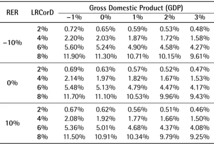
The sign of the coefficient corresponding to real exchange rate is negative, which means that an increase of the real exchange rate would decrease the percentage of defaulted credits. This result might seem counterintuitive. However, we note that in the Corporate Credit category we can find companies selling non-tradable goods, and companies selling tradable goods; the latter ones would increase their capacity to pay from an increase of the real exchange rate. This result indicates that there is a greater proportion of companies selling tradable goods in the Corporate Credit in American Dollars category, meaning that currency mismatch is not very relevant.
Table 7.Corporate Credit in American Dollars: First Model. Stress Test.
RER LRCorD −1% Gross Domestic Product (GDP)0% 1% 2% 3%
−10%
2% 0.72% 0.65% 0.59% 0.53% 0.48%
4% 2.20% 2.03% 1.87% 1.72% 1.58%
6% 5.60% 5.24% 4.90% 4.58% 4.27%
8% 11.90% 11.30% 10.71% 10.15% 9.61%
0%
2% 0.69% 0.63% 0.57% 0.52% 0.47%
4% 2.14% 1.97% 1.82% 1.67% 1.53%
6% 5.48% 5.13% 4.79% 4.47% 4.17%
8% 11.70% 11.10% 10.53% 9.96% 9.43%
10%
2% 0.67% 0.62% 0.56% 0.51% 0.46%
4% 2.08% 1.92% 1.77% 1.66% 1.50%
6% 5.36% 5.01% 4.68% 4.37% 4.08%
8% 11.50% 10.91% 10.34% 9.79% 9.25%
3.3.2. Second Model
The second model is fitted using Unemployment Rate, (6-months lagged) Nominal Exchange Rate, and dummy variable D2009.
This model has a good predictive power. However, the economic interpretation of the coefficients for the selected macroeconomic variables is not very clear. One possible interpretation is that companies selling non-tradable goods have their clients in the domestic market, meaning that an increase of the unemployment rate would drastically decrease the demand for goods, leading to an increase of credit risk. Moreover, companies selling tradable goods may have a large proportion of sells in the domestic market, and thus being affected in case of an increase of the unemployment rate.
This results could be improved if we are able to distinguish between companies selling tradable goods and non-tradable goods.
The results for the linear regression are shown in Table Tabela 8.
Chi-square normality test for the residuals yields a p-value of 0.4498, so normality of the residuals hypothesis is not rejected.
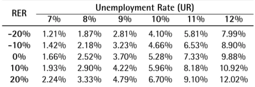
We are able to fit the one-factor model. The results are shown in Tabela 9. Again, for this case, the Unemployment Rate is the variable with largest impact on the probability of default.
Table 8.Corporate Credit in American Dollars: Second Model. Linear regression.
Coefficients Typical Deviation Statistic t p-value
Constant −3.7114 0.0583 −63.61 0.00
UR 17.0033 0.5685 29.90 0.00
NER (−6) 0.6123 0.0772 7.93 0.00
D2009 −0.2251 0.0694 −3.24 0.00
3.3.3. Third Model
Table 9.Corporate Credit in American Dollars: Second Model. The log-likelihood is −4,002.69.
Coefficients
Constant −3.5621
UR 16.0535
NER (−6) 0.6430
D2009 −0.2694
ρ 0.0401
Table 10.Corporate Credit in American Dollars: Second Model. Stress Test.
RER 7% 8%Unemployment Rate (UR)9% 10% 11% 12%
-20% 1.21% 1.87% 2.81% 4.10% 5.81% 7.99%
-10% 1.42% 2.18% 3.23% 4.66% 6.53% 8.90%
0% 1.66% 2.52% 3.70% 5.28% 7.33% 9.88%
10% 1.93% 2.90% 4.22% 5.96% 8.18% 10.92%
20% 2.24% 3.33% 4.79% 6.70% 9.10% 12.02%
Nominal Exchange Rate, Gross Domestic Product, Country Risk and the dummy variable D2009. The results for the linear regression are shown in Tabela 11.
Chi-square normality test for the residuals yields a p-value of 0, so normality of the residuals hypothesis is rejected. This means that it is not adequate to fit the one-factor model using this subset of macroeconomic variables.
Table 11.Corporate Credit in American Dollars: Third Model. Linear Regression.
Coefficients Typical Deviation Statistic t p-value
Constant 0.4013 0.1752 2.29 0.02
NER (−6) 0.9818 0.0852 11.52 0.00
GDP −0.0225 0.0013 −17.40 0.00
CR 5.2724 0.9609 5.49 0.00
D2009 −0.5642 0.0786 −7.18 0.00
3.3.4. Corporate Credit in American Dollars. Conclusions
Three models were fit for the Corporate Credit in American Dollars category. The first model has a very clear economic interpretation and a good transmission of the macroeconomic variables, but it has a poor prediction power. The second model has a high prediction power, but economic interpretation is not so clear. The third model has average prediction power and economic interpretation, but the non-normality of the residuals does not allow us to fit a one-factor model for this subset of macroeconomic variables.
3.4. Corporate Credit in National Currency – Consumer Credit in American Dollars
the results for the selected model and two alternative models, as it was done in section 3.2.
3.4.1. Corporate Credit in National Currency
The selected macroeconomic variables for the main model are Unemployment Rate and Lending Rate for Corporations in Uruguayan Pesos. Some evidence of errors in the data were found for some months, so we chose to use a dummy variableDUMMY to take those errors into account. The results for the main
model and two alternative models are shown in Tabela 12.
Table 12. Corporate Credit in National Currency. Maximum likelihood −3,543.83, −3,563.75 and −3,602.89 re-spectively.
Model Alternative 1 Alternative 2
Coefficients Coefficients Coefficients
Constant −2.9412 Constant 1.9266 Constant −1.0015
UR 7.4698 RER −0.0092 LRCorP 0.7974
LRCorP 0.5930 GDP −0.0241 GPD −0.0103
DUMMY 0.7026 DUMMY −0.2320 DUMMY −0.2069
ρ 0.0000 ρ 0.0427 ρ 0.0364
We note, from Tabela 13, that Unemployment Rate is selected again for a Corporate Credit cate-gory, despite of being a macroeconomic variable related to the domestic demand of goods. The lending rate is positively correlated with credit risk, and the value ofρshows that the non-observable
macroeco-nomic factor is not relevant for this category, possibly reflecting a lower credit risk arising from currency mismatch for this category.
Table 13.Corporate Credit in National Currency: Main Model. Stress Test.
LRCorP 7% 8%Unemployment rate (UR)9% 10% 11% 12%
10% 2.47% 2.94% 3.47% 4.08% 4.77% 5.56%
15% 2.65% 3.14% 3.71% 4.35% 5.08% 5.89%
20% 2.83% 3.35% 3.95% 4.63% 5.39% 6.24%
25% 3.03% 3.58% 4.21% 4.92% 5.72% 6.60%
3.4.2. Consumer Credit in American Dollars
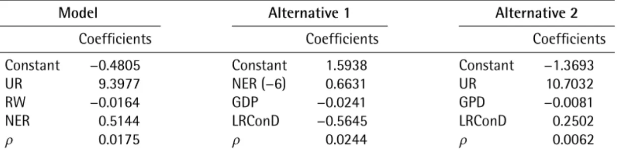
For this category, the selected macroeconomic variables for the main model are Unemployment Rate, Real Wage Index, and (6-month lagged) Nominal Exchange Rate. The results for the main model and two alternative models are shown in Tabela 14.
As in the Consumer Credit in National Currency category, from Tabela 15, we conclude that Unem-ployment Rate is again a relevant macroeconomic variable. We also note that an increase of the Nominal Exchange Rate will lead to an increase of credit risk, reflecting that the income of most families is in national currency.
4. CONCLUSIONS
Table 14. Consumer Credit in American Dollars. Maximum likelihood −10,337.35, −10,360.79 and −10,400.21 respectively.
Model Alternative 1 Alternative 2
Coefficients Coefficients Coefficients
Constant −0.4805 Constant 1.5938 Constant −1.3693
UR 9.3977 NER (−6) 0.6631 UR 10.7032
RW −0.0164 GDP −0.0241 GPD −0.0081
NER 0.5144 LRConD −0.5645 LRConD 0.2502
ρ 0.0175 ρ 0.0244 ρ 0.0062
Table 15.Consumer Credit in American Dollars: Main Model. Stress Test.
NER RW 7% 8% Unemployment Rate (UR)9% 10% 11% 12%
−10%
−2% 6.65% 7.91% 9.32% 10.90% 12.63% 12.63%
−1% 6.40% 7.62% 9.00% 10.54% 12.24% 14.08%
0% 6.14% 7.34% 8.69% 10.19% 11.85% 13.66%
1% 5.91% 7.06% 8.38% 9.85% 11.48% 13.25%
2% 5.67% 6.80% 8.08% 9.51% 11.11% 12.85%
0%
−2% 7.32% 8.66% 10.17% 11.83% 13.63% 15.58%
−1% 7.05% 8.37% 9.83% 11.45% 13.22% 15.14%
0% 6.78% 8.06% 9.49% 11.08% 12.81% 14.71%
1% 6.52% 7.77% 9.16% 10.72% 12.43% 14.28%
2% 6.27% 7.46% 8.84% 10.37% 12.04% 13.87%
10%
−2% 8.04% 9.47% 11.06% 12.80% 14.68% 16.69%
−1% 7.75% 9.14% 10.70% 12.40% 14.26% 16.24%
0% 7.46% 8.82% 10.34% 12.02% 13.84% 15.80%
1% 7.18% 8.51% 9.99% 11.64% 13.43% 13.35%
2% 6.91% 8.21% 9.66% 11.26% 13.02% 14.92%
under a threshold dependent on some macroeconomic variables, meaning that the value of the threshold is updated based on the macroeconomic environment of the economy.
We focused mostly on the two most important categories for Uruguayan economy, which are Con-sumer Credit in National Currency and Corporate Credit in American Dollars. Additionally, we present the results for the two other categories, which are Consumer Credit in American Dollars (2% of total bank credits) and Corporate Credit in National Currency (12% of total bank credits).
For the Consumer Credit in National Currency category, we obtain a very appropriate model both form the point of view of predictive power and from the point of view of economic intuition. The selected macroeconomic variables are the unemployment rate, the real interest rate and the inflation rate. A further possible improvement to model this category is to discriminate the residential mortgage loans from the total consumer credit.
on an index of economic activity, the interest rate charged by the banks, and the real exchange rate. Nevertheless, it is thought that this model must be improved by assessing the credit risk by economic sectors.
We observe that all the models confirm a strong relationship between the macroeconomic envi-ronment and the quality of the loan portfolios of the banking system. Therefore, a possible application of these models is the stress tests referred in Basel II, which could be used both to assess the stability of the financial system as a whole, and to assess the capital level of each institution as its capacity to face adverse shocks. We present the stress tests for all categories, which show credit default probabilities for different economic scenarios.
REFERENCES
Bank of Japan. (2007, September).Financial system report(BOJ Report). Bank of Japan. Retrieved from https://www
.boj.or.jp/en/research/brp/fsr/data/fsr07b.pdf (Box 8: The Framework for Macro Stress-Testing of Credit Risk Incorporating Transition in Borrower Classifications, pp.44–45)
Barone-Adesi, G., Gagliardini, P., & Urga, G. (2000, October). Homogeneity hypothesis in the context of asset
pricing models: The quadratic market model[Cass Business School Research Paper]. Retrieved from https:// doc.rero.ch/record/5394/files/1_fin0102.pdf
Bluhm, C., & Overbeck, L. (2003). Systematic risk in homogeneous credit portfolio. In G. Bol, G. Nakhaeizadeh,
S. T. Rachev, T. Ridder, & K.-H. Vollmer (Eds.),Credit risk: Measurement, evaluation and management(pp.
35–48). Heidelberg: Physica-Verlag HD. doi: 10.1007/978-3-642-59365-9_2
Bunn, P., Cunningham, A., & Drehmann, M. (2005, June). Stress testing as a tool for assessing systemic risks.
Finan-cial Stability Review,18, 116–126. Retrieved from http://www.bankofengland.co.uk/archive/Documents/ historicpubs/fsr/2005/fsrfull0506.pdf
Caicedo Cerezo, E., Bielsa, M. M. C., & Casanovas Ramón, M. (2011). medición del riesgo de crédito
medi-ante modelos estructurales: Una aplicación al mercado colombiano. Cuadernos de Administración
(Bogotá),24(42), 73–100. Retrieved from http://www.scielo.org.co/scielo.php?script=sci_abstract&pid=
S0120-35922011000100004
Céspedes, J., & Martín, D. (2002, January).The two factor model for credit risk: A comparison with the BIS II one
factor model.
Cipollini, A., & Missaglia, G. (2005, Febraury).Business cycle effects on portfolio credit risk: Scenario generation
through dynamic factor analysis.SSRN. doi: 10.2139/ssrn.665724
Coletti, D., Lalonde, R., Misina, M., Muir, D., St-Amant, P., & Tessier, D. (2008, June). Bank of Canada participation
in the 2007 FSAP Macro Stress-Testing Exercise.Financial System Review(Bank of Canada). Retrieved from
http://www.bankofcanada.ca/wp-content/uploads/2012/01/fsr-0608-coletti.pdf
Duffie, D., & Singleton, K. J. (1997). An econometric model of the term structure of interest-rate swap yield. The
Review of Financial Studies,52(4), 1287–1321. doi: 10.1111/j.1540-6261.1997.tb01111.x
Geske, R. (1977). The valuation of corporate liabilities as compound options.Journal of Financial and Quantitative
Analysis,12(4), 541–552.
Hamerle, A., Leibig, T., & Scheule, H. (2004). Forecasting credit portfolio risk(Discussion Paper No. 01/2004).
Frankfurt am Main: Deutsche Bundesbank. Retrieved from https://www.bundesbank.de/Redaktion/EN/ Downloads/Publications/Discussion_Paper_2/2004/2004_02_01_dkp_01.pdf
Jakubík, P. (2005). Macroeconomic credit risk model. In Czech National Bank (Ed.),Financial stability report(pp.
Jakubík, P. (2007, March). Credit risk in the Czech economy(Working Paper No. 11/2007). Prague: FSV–IES. Retrieved from http://ies.fsv.cuni.cz/sci/publication/show/id/2031/lang/en
Jarrow, R., & Turnbull, S. (1995). Pricing derivatives on financial securities subject to credit risk. Journal of
Finance,50(1), 53–85. doi: 10.1111/j.1540-6261.1995.tb05167.x
Jiménez, G., & Mencía, J. (2007). Modelling the distribution of credit losses with observables and latent factors
(Documentos de Trabajo No. 0709). Madrid: Banco de España. Retrieved from http://www.bde.es/informes/ be/docs/dt0709e.pdf
J.P. Morgan & Co. (1997).CreditMetrics™(Technical Document). New York: J.P. Morgan & Co.
Lucas, A., & Klaassen, P. (2003). Discrete versus continuous state switching models for portfolio credit risk
(Discussion Paper No. 2003-075/2). Amsterdam: Tinbergen Institute. Retrieved from http://www.tinbergen .nl/discussionpaper/?paper=431
Luo, X., & Shevchenko, P. V. (2013). Markov chain monte carlo estimation of default and recovery: Dependent
via the latent systematic factor.arXiv.org. Retrieved from https://arxiv.org/abs/1011.2827
Merton, R. (1974). On the pricing of corporate debt: The risk structure of interest rates. Journal of Finance,22,
449–470.
Molins, J., & Vives, E. (2016). Model risk on credit risk.Risk and Decision Analysis,6(1), 65–78. doi:
10.3233/RDA-150115
Rosch, D. (2003). Correlations and business cycles of credit risk: Evidence from bankruptucies in Germany.
Finan-cial Market and Portfolio Management,17(3), 309–331.
Rosch, D. (2005). An empirical comparison of default risk forecast from alternative credit rating philosophies. International Journal of Forecasting,21, 37–51.
Vasicek, O. (1987, February).Probability of loss on loan portfolio(Tech. Rep.). San Francisco, CA: KMV Corporation.
Virolainen, K. (2004).Macro stress testing with a macroeconomic credit risk model for Finland(Discussion Paper
No. 18·2004). Helsinki: Suomen Pankki (Bank of Finland). Retrieved from http://www.suomenpankki.fi/en/