Speculative attacks on debts and optimum currency area: a welfare analysis

Nº 514 ISSN 0104-8910

Speculative attacks on debts and optimum currency area: A

w elfare analysis

Aloisio Araujo M árcia Leon

Speculative Attacks on Debts and Optimum

Currency Area:

A Welfare Analysis

1

Aloisio Araujo

and Marcia Leon

November 14, 2003

1_{We are grateful to Marcio Nakane, Ivan Pastine and other participants at the workshop}

BACEN-USP de Economia Monetária, at the 2003 North American Summer Meetings of the Econometric Society and at the 6th Annual Conference of the Centre for the Study of Globalisation and Regionalisation, University of Warwick, for their comments on this paper. Furthermore, we would like to thank the remarks received from Affonso Pastore, Arilton Teixeira, Carlos Hamilton Araujo, Helio Mori, Ilan Goldfayn, Peter Kenen, Renato Fragelli, Ricardo Cavalcanti, Roberto Ellery and Timothy Kehoe on previous versions of this work. The views expressed here are those of the authors and do not necessarily reflect those of Banco Central do Brasil or its members.

2_{Escola de Pós-Graduação em Economia (Fundação Getulio Vargas) and Instituto de}

Matematica Pura e Aplicada. E-mail: aloisioa@fgv.br; aloisio@impa.br

Abstract

Traditionally the issue of an optimum currency area is based on the theoretical underpinnings developed in the 1960s by McKinnon [13], Kenen [12] and mainly Mundell [14], who is concerned with the benefits of lowering transaction costs vis-à-vis adjustments to asymmetrical shocks. Recently, this theme has been reappraised with new aspects included in the analysis, such as: incomplete markets, credibility of monetary policy and seigniorage, among others. For instance, Neumeyer [15] develops a general equilibrium model with incomplete asset markets and shows that a monetary union is desirable when the welfare gains of eliminating the exchange rate volatility are greater than the cost of reducing the number of currencies to hedge against risks.

In this paper, we also resort to a general equilibrium model to evaluatefinancial aspects of an optimum currency area. Our focus is to appraise the welfare of a country heavily dependent on foreign capital that may suffer a speculative attack on its public debt. The welfare analysis uses as reference the self-fulfilling debt crisis model of Cole and Kehoe ([6], [7] and [8]), which is employed here to represent dollarization. Under this regime, the national government has no control over its monetary policy, the total public debt is denominated in dollars and it is in the hands of international bankers. To describe a country that is a member of a currency union, we modify the original Cole-Kehoe model by including public debt denominated in common currency, only purchased by national consumers. According to this rule, the member countries regain some influence over the monetary policy decision, which is, however, dependent on majority voting. We show that for specific levels of dollar debt, to create inflation tax on common-currency debt in order to avoid an external default is more desirable than to suspend its payment, which is the only choice available for a dollarized economy when foreign creditors decide not to renew their loans.

Keywords: dollarization, optimum currency area, speculative attacks, debt crisis, sunspots

1

Introduction

Emerging market economies of Latin America and Southeast Asia accumulated high

levels of external debt in the 1990’s. The sharp demand for foreign credits helped

sustain stabilization programs and strengthen the value of national currencies.

Reversal of market expectations and contagion effects changed this environment,

causing financial crisis for some of these economies. Argentina and Russia actually

defaulted, while Mexico, Korea, Thailand, Hong Kong and Brazil experienced severe

speculative attacks.

With this background in mind, we make an extension to the Cole and Kehoe (

[6], [7] and [8]) model on self-fulfilling debt crisis to describe an economy for which

there is positive probability of defaulting on its external debt, but also belongs

to a currency union. Under this monetary regime, a default may be avoided by

inflation of the common currency, which, however, incurs costs in terms of a fall in

productivity. Besides, the decision to inflate depends on majority voting and the

welfare of a country with low weight in the voting system is adversely affected by

antagonistic choices. We also try to evaluate the contagion among members that

results from a loss in confidence of international bankers towards one country being

passed on to another.

One of the advantages of the Cole-Kehoe methodology is to do welfare analysis.

We use their approach to evaluate the expected welfare of a member country of

a monetary union constituted of two partners. We do simulations for Brazil for

the period from June 1999 until May 2001, supposing that it has high and low

weight in the voting system of a monetary union. We compare the results from this

model with the expected welfare given by the original Cole-Kehoe model, which we

characterize as being a dollarization regime, and also to a model with local currency

and central bank under political influence by its government. Our main result is

that for a low-weight country with dollar debt in the crisis zone, local currency

regime may be a better choice than the common-currency one, even if the central

by its government. If this dependence is not too strong, the possibility to inflate, at

its own will, to avoid a default under local-currency regime produces higher welfare

than the need to wait on majority decision as is the case in the other regime. For the

low-weight country, common currency is superior to dollarization, because under the

former regime it is possible to avoid a default through inflation, while this alternative

is absent in the latter.

On a more methodological ground, this paper can be viewed as part of

the literature on general equilibrium with bankruptcy, which asserts that in an

incomplete market situation the introduction of the possibility of bankruptcy can

be welfare enhancing (see Dubey, Geanakoplos and Zame [10], for static economies,

and Araujo, Páscoa and Torres-Martínez [3], on infinite horizon economies). The

introduction of common currency can give rise to the possibility of a better

bankruptcy technology through inflation than just the repudiation of the external

debt, which can be quite costly.

2

The Cole-Kehoe Model

Cole and Kehoe developed a dynamic, stochastic general equilibrium model in which

they consider the possibility of a self-fulfilling crisis of the public debt occurring. The

crisis takes place when the government needs to renew its loans and the international

bankers, realizing that it will not pay them back, decide to suspend them. Given

this decision, the government defaults, confirming the creditors’ initial beliefs.

2.1

Basic Assumptions

The basic assumptions of the original Cole-Kehoe model are: one good produced

with capital, k, inelastic labor supply, and price normalized at one dollar; three

participants – national consumers, international bankers and the government; one

exogenous sunspot variable, ζ, which describes the bankers confidence that the

government will not default. The sunspot is supposed independent and identically

confidence is below the critical valueπ is equal to the probability of a self-fulfilling

debt crisis occurring, i.e. P (ζ _≤π) =π. The model also assumes a stock of dollar

debt, B, supposed to be completely in the hands of the bankers and probabilityπ of

no rollover if its level lies in the crisis zone. If the government defaults, it is always

total. The decision to default is characterized by the government’s decision variable,

z, equal to zero. Otherwise, it is equal to one.

In the original model, the representative consumer maximizes expected utility

max

ct,kt+1

E

∞ X

t=0

βt[%ct+v(gt)] (1)

subject to the budget constraint

ct+kt+1−k_t≤(1−θ) [a_tf(k_t)−δk_t]

and given initial capital

k0 >0

At instant t, the consumer chooses how many goods to save for next period, kt+1, and to consume presently, ct. The utility has two parts: a linear function of private

consumption, %ct, and a logarithmic function v of government spending, gt. The

term % is the weight of the utility of private consumption relative to the utility of

public consumption. The right hand side of the budget constraint corresponds to

the consumer’s income, after taxes (θ is the tax rate) and capital depreciation, given

byδ. The termatis essential to the Cole-Kehoe model. It is the productivity factor.

If the government defaults on its debt, then the economy suffers a permanent drop

in national productivity, at =α,0<α<1. Otherwise, at is equal to one.

The problem of the representative international banker is analogous to the

consumer problem, except that the instantaneous utility excludes the term related

to government spending, and consists of

max

xt,bt+1

E

∞ X

t=0

βtxt (2)

s.t.

and given a initial amount of public debt

b0 >0

At time t, the bankers choose how many goods to consume, xt, and the amount of

government bonds to buy,bt+1. The left hand side of the budget constraint shows the

expenditure on new government debt, whereq∗

t is the price of one-period bonds that

pay one unit of the good at maturity if the government does not default. The right

hand side includes the revenue received from the bonds purchased in the previous

period. The decision variablez indicates government default (z = 0) or not (z = 1).

If it defaults, then the bankers receive nothing.

The government is assumed benevolent, in the sense that it maximizes the

welfare of national consumers, and with no commitment to honor its obligations. Its

decision variables are: new debt,Bt+1, whether or not to default,zt, and government

consumption, gt. It has a budget constraint given by

gt+ztBt≤θ[atf(Kt)−δKt] +q∗tBt+1 (3)

where the expenditure, on the left hand side of expression (3), refers to current

consumption and the payment of its debt; while the revenue, on the right hand side,

includes taxes and the selling of new debt. The government is also assumed to have a

strategic behavior since it foresees the optimal decision of the participants, including

its own, ct, kt+1, q∗t, zt and gt, given the initial aggregate state of the economy, st,

and its choice of Bt+1.

The timing of actions within a periodt is (the subscript t is omitted):

• the sunspot ζ is realized and the aggregate state is s= (K, B, a−1,ζ);

• the government, given the price function q∗ _=q∗_{(s, B}0_{), choosesB}0_;

• the bankers decide whether or not to purchase B0_;

• the government chooses whether or not to default, z, and how much to

• finally, consumers, given a(s, z), decide aboutc andk0_.

2.2

A Recursive Equilibrium

In the construction of a recursive equilibrium, the first step is to characterize the

behavior of the consumers and bankers. The optimal accumulation of capital, k0_,

may take three valueskn _{> k}π _{> k}d_{, depending on the consumers’ expectation about}

the productivity factor in the next period, E[a0_{]. When the expectation is equal to}

one, k0 _{equals k}n_{. If consumers expect a debt crisis next period with probability π,}

then E[a0_{] equals 1−π+πα and they choose k}π_{. Finally, when consumers know}

that the government has defaulted or will default for sure, they expect a drop in the

productivity factor toαandk0 _iskd_{. Analogously, the price that bankers pay for the}

new debt may take three values, β,β(1−π) and0, depending on their expectation

of whether or not the government will default next period, since q∗ _{= βE[z}0_{]. For}

example, if bankers expect no default ( E[z0_{] = 1), then q}∗ _{is β.}

The second step in the construction of a recursive equilibrium is to define the

crisis zone with probability π. For a given maturity of government bonds, the

crisis zone is the debt interval for which a crisis can occur with probability π. For

one-period government bonds and aggregate state s = (kπ_{, B,1,ζ), such that there}

is probability π of a default, the crisis zone is given by

³

b(kn), B(kπ,π)i

The lower limit, b(kn_{), is the highest debt level such that the government’s payoff}

of not defaulting, Vn

g , is greater than the payoff of defaulting, Vgd, when it does not

obtain new external loans (the second argument, B0_{, and the third, q}∗_{, are zero in}

the condition below). This restriction is called theno-lending condition and is given by the expression

V_gn(s,0,0)≥V_gd(s,0,0)

On the other hand, the upper limit,B(kπ_{,π), is the highest debt level such that the}

debt at positive price β(1−π). This condition is written as

V_gπ(s, B0_{,β(1−π))≥V}d

g(s, B0,β(1−π))

Given these limits of the crisis zone, if the government chooses new dollar debt

below the crisis zone, B0 _{≤ b(k}n_{), then bankers will always renew their loans. If}

new dollar debt is inside the crisis zone and the realization of the sunspot is such

that the international bankers are confident that the government will honor its

obligations, then the creditors rollover the debt and are aware of a possible default

with probability π next period. Finally, if the new debt is above the crisis zone,

B0 _{> B(k}π_{,π), then there will be default for sure in the following period and the}

bankers purchase no new debt.

2.3

Numerical Exercise

Using their model, Cole and Kehoe [6] did a numerical exercise for Mexico for the

eight months before the 1994-95 crisis. The parameters they used are: an average

maturity of eight months for the public debt; capital share, ν, equal to 0.4 applied

to the production function f(k) = Akν _{and total productivity factor, A = 2.0; tax}

rate, θ = 0.2; drop in productivity after default of0.05, meaningα= 0.95;discount

factor, β = 0.97; depreciation factor,δ = 0.05; and probability of default,π = 0.02,

corresponding to one minus the ratio of the interest rate on U.S. Treasury bills and

on Mexican dollar-indexed bonds (Tesobonos) with equal maturities, given by

π = 1₋ (1 +r∗)

(1 +r) (4)

One result of their simulation is the government debt policy function. For a

given current debt level, it determines the amount of new debt the government

chooses. Another result of their simulation is the crisis zone for different maturities

of the public debt. They show that Mexico’s domestic government debt of 20%,

We do a similar exercise for Brazil for the 24-month period from June 1999 to

May 2001. The parameters we use are the following: average maturity of public

debt of 24 months; capital share, ν = 0.5; tax rate, θ = 0.3; probability of default,

π = 0.06; drop in national productivity after default equal to the Mexican one

(α = 0.95); and depreciation factor, δ= 0.24.

The two-year interval is equal to the average maturity period of Brazilian

government debt. We assume that the average maturity of debt denominated in

local currency follows the average maturity for debt indexed by the Selic rate (the

basic rate set by Banco Central do Brasil), while, for debt denominated in dollar is

the same as for dollar-indexed bonds. Both average maturities are approximately 24

months for the period under study. Araujo and Leon ([2], Tabela 3) obtain that net

public sector debt denominated or indexed to the dollar is 0.20 relative to GDP and,

denominated in Brazilian money, 0.30, during June 1999 to May 2001. As shown in

Figure 1, if we make the strong assumption that total Brazilian public sector debt

could suffer a run and is subject to the mood of the international creditors, then,

for an average maturity of 24 months, it would be inside the crisis zone.

3

A Model with Common Currency

We modify the original Cole-Kehoe model to assess the welfare of an economy that

belongs to a currency union. The currency union model is mainly characterized

as one with two currencies (the common one, such as the Euro, and the dollar),

I member countries and a central government, equivalent to the Council of the

European Union, constituted as the decision-making body for all members. Each

country i, i = 1, . . . , I, issues debt in the two currencies: dollar, Bi_{, and common}

currency, Di_{. Since there is debt denominated in common currency, it is possible for}

the central government to collect inflation tax, but this decision depends on majority

3.1

Basic Assumptions

The currency union model is very similar to the original Cole-Kehoe model. The

basic assumptions are: participants in the market for the reference good – national

consumers for I countries, international bankers, national government from I

countries and the central government; the price of the good equals one dollar, or pt

units of the common currency, in all member countries; each country i issues debt

denominated in dollars, Bi_{, which is only acquired by international bankers, there}

is probability πi _{of no rollover if its level is in the crisis zone and any suspension in}

payment is always total; also, each country i issues debt denominated in common

currency, Di_{, which is only taken up by consumers from this country, there is always}

credit rollover and repayment may be suspended partially.

Analogous to the original model, the decision to default on dollar debt is

characterized by the national government’s decision variable, zi_{, being equal to zero}

and a permanent fall in national productivity, ai_{, to α}i_{, 0 < α}i _{< 1. Meanwhile,}

the decision whether or not to create inflation tax on common-currency debt is

described by the central government decision variable, ϑu_t, which may take one of two values: 1 or φ = 1

1 +χ, 0 < φ < 1 and χ, the inflation rate. If the central

government decides for no inflation tax, then the common currency bond pays one

good,υu _{= 1, as the dollar bond does. Otherwise, it pays less than one unit,υ}u _=φ.

The national government obtains additional revenue by the lower real return paid for

the common-currency bonds held by consumers after the central government decision

to inflate. If there is inflation, consumers receiveφgoods per common-currency bond

and believe that the government will henceforth start paying this quantity of goods

per bond, while country i is affected by a permanent fall in productivity, ai_{, toα}φ_,

which is related to the rate of inflation tax chosen. Therefore, the decision to inflate

brings a cost to the member countries in terms of lower productivity, despite the

benefit of the extra revenue to avoid an external default. An alternative approach

to include inflation cost is to suppose a reduction in consumer’s utility, but this is

Uncertainty is included in the model by three sunspot variables: two for each

country i, ζi and ηi_{, and one for the union, η}u_{. The sunspot ζ}i_{, as in the original}

Cole-Kehoe model, describes the bankers’ confidence that government i will not

default on its external debt. We assume thatζi, from countryi, is affected by sunspot

ζj from another countryjbelonging to the currency union in the following way: first, we suppose that the probability that bankers’ confidence in governmentiis below the

critical valueπi_{given that their confidence in governmentj is higher than the critical}

valueπj _isπi_{, whereπ}i _{is the probability of a self-fulfilling dollar debt crisis occurring}

in countryigiven that there is no crisis in countryj, i.e. P³ζi ≤πi _|ζj

>πj´_=πi_;

and second, we assume analogously thatP³ζi _≤πi _|ζj

≤πj´_=πij_{, whereπ}ij _{is the}

the probability of a self-fulfilling dollar debt crisis occurring in countryi, given an

external debt crisis occurred in countryj. Supposing a currency union with only two

countries, Table 1 and Table 2, in the Appendix, show the conditional probability

of ζ2

givenζ1

and their joint probability.

The other sunspot for country i, ηi_{, is conditional on ζ}i

and describes the

confidence that consumers from country i have that the central government will

honor its obligations regarding payment of the common currency bonds. We assume

that the probability that the confidence of consumers from country i is below the

critical valueξi, given that international bankers have little confidence in government

i, is ξi, i.e. P(ηi _{≤ ξ}i _{| ζ}i

≤ πi_{) = ξ}i_{, where ξ}i _{is the probability that government}

i votes for inflation tax. Table 3 shows the conditional probability of ηi _{given ζ}i

.

The national government’s choice about inflation influences the central government

decision according to the weight of each country in the voting system, ϕi_{. If the}

majority of member countries is not under a speculative attack, then the realization

of the sunspots ηi _{for alli is irrelevant, since there is no reason to inflate.}

Finally, the sunspotηu _{gathers allη}i_{and describes the confidence that consumers}

from the union have about the central government decision not to inflate the common

currency. We assume that the probability that the confidence of consumers from the

the majority of countries is below the critical value ξi, is ξu. We define ξu as the average ξi for all member countries according to their weight in the voting system and it corresponds to the probability that the members vote in favor of inflation

tax.

Table 4 shows, for a currency union constituted of two countries, the conditional

probability of ηu _{given that the confidence of the consumers from each country,}

η1

and η2

, are affected by the low confidence of the international bankers. The

realization of the sunspots η1

and η2

may be symmetrical or asymmetrical. In

case of symmetry, the consumers’ confidence may be both small with η1

≤ ξ1 and

η2

≤ξ2

(and inducing national governments 1 and 2 to vote in favor of inflating the

common currency) or both big with η1

> ξ1 and η2

> ξ2 (and both governments

voting against inflation) . If η1

and η2

are small, then ηu _{is also small (η}u _{≤ ξ}u_).

The conditional probability that ηu _{≤ ξ}u

, given that η1

and η2

are symmetrical, is

ξu, which is defined as the weighted average of ξ1

and ξ2

, as shown in cell (1,1) of

Table 4. In case of asymmetry, we assume that country 1 has the highest weight

in the voting system and, consequently, the union’s confidence reflects the one from

country 1. According to this hypothesis,ξuuis defined as the conditional probability that the union’s confidence is small, ηu _{≤ ξ}u_{, given that the consumers’ con}

fidence

from country 1 is also small, η1

≤ ξ1, and from country 2 is big, η2

> ξ2. On the

other hand, (1₋ξuu) is the conditional probability that the union’s confidence is big when the consumers’ confidence from country 1 is big and, from country 2, is

small .

Table 5 presents the joint probability of the three sunspots η1 , η2

andηu_{. The}

probability si refers to the joint probability of symmetry (s) between η1

andη2 and

inflation (i),snirefers to symmetry (s) and no inflation (ni). Analogously, we define

the probabilities asi andasni, for the case of asymmetry (a).

The different realizations of ηi _{for each country correspond to the political risk}

that national government i faces in adopting a common currency. The realization

and the central government are in harmony regarding price versus output stability.

Antagonistic types of national governments can result in different preferences

regarding the conduct of common monetary policy. This same question is analyzed

by Alesina and Grilli [1], but using a different theoretical approach.

Figure 2 is a tree diagram for two countries in a currency union in one period.

The branches of the tree indicate the probabilities that the market participants face

before realization of the sunspot variables, when the initial state is such that there

has not been inflation tax and both countries may default on their dollar debts.

3.2

Description of Participants

At timet, the representative consumer from countryimaximizes the expected utility,

given by expression (1), subject to the new budget constraint

ci_t+ki_t+1−k

i

t+qtidit+1 ≤

³

1₋θi´ hai_tf³k_ti´₋δik_tii+ϑu_tdi_t

Besideski

t+1 andcit, the representative consumer from countryichooses the amount

of new common-currency debt, di

t+1. The common-currency debt consists of

zero-coupon bonds maturing in one period that pay one unit of the good if there

is no inflation. Otherwise, it pays φ units. The right-hand side of the budget

constraint includes the expenditure on new common currency debt, qi

tdit+1, and the

left-hand side, the payment of the debt purchased in the previous period, ϑutdit. We

also assume that the consumer holds an amount di

0 of the common-currency debt

initially.

International bankers maximize the expected utility given by the expression (2),

subject to the budget constraint

xt+ I

X

i=1

q_t∗ibi_t+1 ≤x+

I

X

i=1

z_tibi_t

which includes purchase and redemption of dollar debt of the I member countries.

Each banker chooses dollar-denominated bonds of countryiat timet,bi

t+1, and pays

q∗i

At timet, the national government of countryimakes the following choices: new

dollar debt, Bi

t+1, new common-currency debt, Dit+1, whether or not to default on

its dollar debt, zi

t, and current government consumption,git. The budget constraint

at time t is

g_ti+z_tiB_ti+ϑu_tD_ti _≤θihai_tf³K_ti´₋δiK_tii+q_t∗iB_ti+1+q

i tDit+1 which is rewritten as,

g_ti _≤θihai_tf³K_ti´₋δiK_tii₋zi_tB_ti+q_t∗iB_ti+1+ (1−ϑ

u

t)Dti+qtiDit+1−D

i t (5)

where (1₋ϑu_t)Di

t refers to the additional revenue that the national government i

obtains by the lower real return of the common-currency debt held by consumers.

Finally, the central government is also assumed benevolent, since maximizes the

welfare of the consumers from the union. It decides whether or not to inflate the

common-currency debt, ϑu_t, which depends on the decisions of the member countries and their relative influence in the voting system, ϕi_{, i= 1, . . . , I. If the sum of the}

weights of the countries that do not wish to inflate the common currency is greater

than, for example, two-thirds of the total votes, then the central government chooses

ϑu= 1. Otherwise, it choosesϑu =φ. We do not model how the inflationφis chosen. At the initial period, for each country i, the supply of dollar debtBi

0 is equal to the demand for this debt, bi_{0; the supply of common-currency debt D}i

0 is equal to

the demand for this type of debt, di_{0; and the aggregate capital stock per worker,}

Ki

0, is equal to the individual capital stock,k0.i

3.2.1 Timing of actions within a period for country i

• the sunspot variables ζi, ηi _{and η}u _{are realized and the aggregate state of}

economy iis si = (Ki, Bi, Di, a₋i 1,ϑu₋1, ζi,ζj, ηi, ηu);

• the government of countryi, taking the dollar-bond price scheduleq∗i _=q∗i_(si_,

B0i_{) as given, chooses the new dollar debt, B}0i_;

• the international bankers, taking q∗i _{and ϑ}u _{as given, choose whether to}

• the government of countryi, taking the common-currency-bond price schedule,

qi _=qi_(si_,B01

,. . .,B0I_{) as given, chooses the new common-currency debt,D}0i_;

• consumers, considering q∗i_{, q}i _andϑu

as given, decide whether to acquire D0i_;

• the central government decides whether or not to inflate the common currency,

ϑu and national government i decides whether or not to default on its dollar debts, zi_{, and its current consumption, g}i_;

• consumers, taking ai _=ai_(si_{, z}i_,ϑu_{) as given, choosec}i _andk0i_.

3.3

A Recursive Equilibrium

Following the Cole-Kehoe model, we define a recursive equilibrium for one country

belonging to a currency union constituted of two partners. We assume that one

of the countries has the highest weight in the voting system, ϕ1

> 0.5, and call it

country 1. The highest weight means that its choice is actually the decision of the

central government. The other country with weight (1₋ϕ1

) is named country 2.

Our purpose is to define a recursive equilibrium and do welfare analysis for both

countries. First, we describe the behavior of consumers and bankers.

Consumers

At time t, consumers know ϑu_t, gi

t and zti when making their decisions as to cit

andki

t+1 and take these variables as given when deciding on dit+1. The optimization

problem at time t corresponds to

max

ci t,k

i t+1,d

i t+1

ci_t+βEci_t+1

s.t.

ci_t+k_ti+1−k

i

t+qitdit+1 =

³

1−θi´ hai_t f³k_ti´−δik_tii+ϑu_tdi_t

ci_t+1+k

i t+2−k

i t+1+q

i t+1d

i t+2 =

³

1₋θi´ hai_t+1 f

³ k_ti+1

´

−δik_ti+1

i

+ϑu_t+1d

i t+1

ci_t, ci_t+1, k

i t+1, d

i

The first order condition for capital accumulation is the same as in the original

Cole-Kehoe model, given production function f(k) = Akν_{. It depends on the}

consumers’ expectation regarding the productivity of the economy in the following

period, Et

h ai

t+1

i

, as shown in the expression below

ki_t+1 =

("Ã 1 β −1

! 1

1₋θi +δ

i

#

1 Et[ait+1]Aiνi

) 1

νi₋₁

(6)

Moreover, the price that the consumers pay for the new common-currency debt is

given by

qi_t=βEt

h ϑu_t+1

i

For consumers from country 1, the possible choices of capital accumulation

arekπξu

,kπφ_,knφ_,kd_andkn _{and of the price of new common-currency debt areq}πξu

,

qφ _{and q}n_{. National consumers from country 1save k}πξu

, because they expect that

the productivity factor next period,Et[at+1], to beππ21[(si+asi)αφ+ (sni+asni)α]

+π(1−π21

) [ξ1

αφ_{+ (1−ξ}1

)α] + (1−π), whereπis the probability of default from

country 1 and π21

, from country 2 given that country 1 is under crisis. Also, they

pay priceqπξu

whenEt

h ϑu_t+1

i

isππ21

[(si+asi)φ+ (sni+asni)] +π(1−π21

) [ξ1φ +

(1₋ξ1

)] + (1₋π). The choice ofkπξu

andqπξu

is related to an initial state in which

it is possible that one or both countries default on the dollar debt or that a default

can be avoided through an inflation tax on common-currency debt (the initial state

in Figure 2). In the same fashion, consumers decide on kπφ _{when there has been}

inflation tax and it is possible that country1defaults on the dollar debt next period.

Consequently, Et[at+1] = (1−π)αφ +π1α, meaning that the productivity factor is maintained at αφ _{if sunspotζ}1

is such that international bankers renew their loans,

or falls to α otherwise. If the central government decides to inflate, then consumers

pay qφ_{, defined as βφ, for new common-currency debt from then on, regardless of}

the realization of the sunspot ζ1

. The expectation on productivity associated with

capital levels knφ_{, k}d _{and k}n _{are α}φ_{, α and 1, respectively. The capital level k}d _is

chosen if the national government defaults on dollar debt. If the private sector is

there had been inflation tax, knφ _{is the one picked, otherwise, they choose k}n _and

pay price qn_{, defined asβ, for new common-currency bonds.}

For consumers from country2, the possible choices of optimal capital are: kππ2 ξu

,

kπξ1

, kππ21_φ

, kπ2_φ

, knφ_{, k}nφn

, kπ2

, kd _{and k}n_{. The first one in the list refers to the}

optimal choice whenE[at+1] =ππ 21

[(si+asi)αφ_{+(asni+sni)α] +π(1−π}21

)(ξ1αφ₊

1₋ξ1

) + (1₋π)[1₋π2

(1₋α)]. Consumers have this belief when it is possible for one

or both countries to default on the dollar debt or for a default to be avoided through

an inflation tax on common-currency debt in the following period (the initial state

in Figure 4). Also according to these beliefs, consumers from country 2 pay price

qπξu

. On the other hand, when it is possible that only country1defaults or votes for

inflation, then the optimal capital is denoted bykπξ1

, meaning that just the sunspots

ζ1

andη1

matter. Forkπξ1

, E[at+1] corresponds to 1 − π + πsi0 + πasi0 αφ

n

and

the price that consumers from country 2 pay for new common-currency debt is qπξ1

equal to β(1₋π+πsi0 +πasi0φn), where asi0 is the probability of asymmetry and si0 of symmetry between the decisions of the two national governments not to

inflate the common currency, given that consumers from country2would rather not

have inflation for sure. Actually, si0 is equal to³1−ξ1´ andasi0, to ξ1.

The distinction between αφn

and αφ _{is related to the abatement factor of the}

common-currency debt, ϑu, and specifically to the vote of country 2 to inflate. Supposing that the sunspot of country 1 influences country 2, two situations may

happen: sunspot ζ2 matters or not at present, which depends on the level of dollar

debt of government 2. If ζ2

matters and country 1 prefers not to default and votes

for inflation, then the abatement factor ϑu is equal to φ. On the other hand, if

ζ2

does not count and country 1 votes for inflation, then ϑu is φn, indicating that country 2surely chooses no inflation.

Given the initial state of the economy s2

= (kππ2_ξu

, B2 , D2

, a2

−1, ϑ

u

−1, ζ

1 , ζ2

,

ηu_{, η}2

), with a2

−1 = 1, ϑ

u

−1 = 1, ζ 1

≤ π1

, ζ2 ≤ π2 , η1

≤ ξ1 and any η2 , the

central government decides for inflation and both countries do not default on their

external debts, as indicated by the realization of the sunspotsζ1andη1

accumulation of capital for next period may take two values: kππ21

φ_{, if sunspotsζ}1

and ζ2

matter in the following period, with the expectation of the productivity

factor, Et[at+1], equal to (1−π 1

) (1−π2

)αφ _{+ (1−π}1

)π2

α + π1

(1−π21

)αφ ₊

π1

π21

α; or the optimal capital iskπ2_φ

, defined byE[at+1]equal toπ2α+(1−π2)αφ, if sunspotζ2is the only one taken into account by the private sector for the following

period. Again, after inflation, consumers pay a price qφ _{for common currency debt.}

Finally, consumers choosekπ2

, given byE[at+1] = 1−π 2

(1−α), and pay price

β for common currency debt, when consumers from country 2 know that country 1

decided to default instead of inflating.

International Bankers

At timet, international bankers solve

max

xt,b1_t+1,...,bI_t+1

xt+βEt[xt+1]

s.t.

xt+q∗t1b

1

t+1+. . .+q∗

I

t bIt+1 =x+z 1

tb

1

t +. . .+ztIbIt

and the first-order condition for bi t+1 is

qt∗i =βEt

h zit+1

i

The price that external creditors pay for new dollar debt of country 1may take

four values: 0, β, β(1₋π), and q∗πξu

. For new dollar debt issued by government

2, the price that external creditors are willing to pay may take five values: 0, β,

β(1₋π2

),q∗ππ21_φ

andq∗ππ2_ξu

. If the central government has undertaken an inflation

tax and bankers believe that the national governmentiwill default on the dollar debt

with probability πi _{in the following period, they pay β(1−π}i_{) for new dollar debt}

from this country. However, if the national government currently defaults on dollar

debt, then international bankers pay price zero. In case external creditors are sure

that the government will not resort to a dollar debt moratorium, they pay β. For

country1, the priceq∗πξuis defined byEt

h z1

t+1

i

equal toππ21

(si+asi) +π(1−π21

+ (1−π) and, for country 2, the price qππ2 ξu

is related to Et

h z2

t+1

i

= π(1−π21

)

+ (1₋π) (1₋π2

) +ππ21

(si+asi). In both cases, external creditors expect that

one or the other country or both may default on their dollar debt or that a default

can be avoided through an inflation tax on debt denominated in common currency.

Finally,q∗ππ21

φ _{refers to an expectation of default of [π(1−π}21

) + (1−π) (1−π2

)]

and is chosen after the central government has decided to inflate and both sunspots

ζ1 and ζ2 matter.

In the next step to construct an equilibrium, we describe the crisis zone using the

following assumptions: (i) there has not been a debt crisis in any of the countries

of the monetary union, nor partial moratoria of common-currency debt, up to the

initial state (i.e., ai

−1 = 1 for all iandϑ

u

−1 = 1); and (ii) the common-currency debt

is fixed at level D.

3.4

The Crisis Zone

The crisis zone is defined as the dollar debt interval for which the international

bankers attribute positive probability for country i to default on its external debt

in the following period. First, we obtain the crisis zone for the country with the

highest weight in the voting system and afterwards, for the country with the lowest

weight.

Crisis zone for country 1 (country with high weight in voting system)

The crisis zone is given by the interval³b(kn_{, D), B}³_kπξu

, D,π,ξu´i. The lower boundb(kn_{, D)is the highest dollar debt level,B}1

, for which the following restriction

is satisfied in equilibrium:

Vn³s1

,0,0, D,β´_≥Vd³s1

,0,0, D,β´ (7)

where s1

= (kn_{, B}1

, D, 1, 1, ·, ·, ·) is an initial state in which country 1 has not

defaulted on the dollar debt (ai

−1 = 1), the central government has not inflated

the common-currency debt (ϑu₋1 = 1) and the sunspots do not matter. The welfare levelsVn_(s1

, 0, 0, D, β)andVd_(s1

respectively, not to default (superscript n) than to default (superscriptd), even if it

does not sell new dollar bonds at a positive price in the current period. The second

and third positions of the argument of the welfare functions mean that new dollar

debt B01

andq∗1

are zero. The fourth andfifth arguments indicate that new debt in

common currency,D, is sold forβ. This lower bound is obtained in a similar way as

in the original Cole-Kehoe model, except that in the common-currency model the

purchase and payment of common-currency debt is included. The welfare levels are

Vn³s1

,0,0, D,β´=vhθyn₋B1

−(1₋β)Di+ρ[(1₋θ)yn+ (1₋β)D]+β·wnD(0)

wnD(0) = 1

(1−β){v[θy

n

−(1−β)D] +ρ[(1−θ)yn+ (1−β)D]}

yn=A(kn)γ₋δkn

Vd³s1

,0,0, D,β´=vhθynd₋(1₋β)Di+ρh(1₋θ)ynd+kn₋kd+ (1₋β)Di+β·wdD

ynd =αA(kn)γ₋δkn

wdD= 1

(1₋β)

n

vhθyd₋(1₋β)Di+ρh(1₋θ)yd+ (1₋β)Dio

The upper bound of the crisis zone,B(kπξu

,D,π, ξu), is the highest dollar debt for which international bankers extend loans to country 1, given probability πi _for

each member country to default and probability ξu for the central government to inflate in the following period. It is obtained as the highest dollar debt such that the

following restrictions are simultaneously satisfied in equilibrium, given initial state

s1

=(kπ1_ξu

, B1

, D, 1, 1, ζ1 ,ζ2

, η1

), withai

−1 = 1,ϑ

u

−1 = 1

Vπ1ξu³s1

, B01

, q∗1

, D, q1´

≥Vd³s1

, B01

, q∗1

, D, q1´

(8)

Vπ1³s1

, B01

, q∗1

, D,βφ´_≥Vd³s1

, B01

, q∗1

, D,β´ (9)

Condition (8) says that government 1prefers not to default than to default and also

decides for no inflation tax, because the realization of the sunspot ζ1

> π1

is such

that the bankers are confident in government 1 and renew their loans. Restriction

as long as it sells new dollar debt at price q∗1

and new common-currency debt at

price βφ. Under this condition, the realization of the sunspots is ζ1

≤ π1 and

η1

≤ξ1, meaning that the external and internal creditors have lost their confidence in government 1, but it does not default because the central government creates

inflation tax.

Crisis zone for country 2 (country with low in the voting system)

Since we assume that country1always chooses dollar debt inside the crisis zone,

then the crisis zone for country 2 depends on the realization of the sunspots ζ1

andη1

and is denoted by ³b³kπξ1

, D, π, ξ1´

, B³kππ2_ξu

, D, π, π2

, ξ1

, ξ2´i . The

lower bound b³kπξ1

, D, π, ξ1´

is the highest dollar debt for which the following

restriction is satisfied in equilibrium:

Vn³s2

,0,0, D, qπξ1´_≥Vd³s2

,0,0, D, qπξ1´ (10)

where s2

=(kπξ1

, B2

, D, 1, 1, ζ1 , ·, η1

, ·) is an initial state in which country 2 has

not defaulted on the dollar debt (a2

−1 = 1), the central government has not inflated

the common-currency debt (ϑu₋1 = 1) and the sunspots ζ 1

and η1

matter, whereas

ζ2

and η2

do not. The payoffs Vn³_s2

, 0, 0, D, qπξ1´

and Vd³_s2

, 0, 0, D, qπξ1´

refer to the decision of government 2 not to default and to default, even if it does

not sell new dollar bonds at a positive price in the current period. New debt in

common currency is sold for qπξ1

. The caracterization of both payoffs is available

upon request.

The upper limit of the crisis zone for country2,B(kππ2_ξu

, D,π1

,π2

,ξ1

,ξ2

), given

initial state s2

= (kππ2_ξu

, B2

, D, 1, 1, ζ1 , ζ2

, η1 , η2

) is constructed analogously to

the crisis zone of country1. It corresponds to the highest dollar debt level for which

the following three restrictions are satisfied simultaneously:

Vππ2ξu³s2

, B2₀

, q∗ππ2ξu, D, qπξu´_≥Vd³s2

, B2₀

, q∗ππ21ξu, D, qπξu´ (11)

Vππ21φ³s2

, B2₀

, q∗ππ21φ, D,βφ´≥Vd³s2

, B2₀

Vπ2³s2

, B2₀

,β³1−π2´

, D,β´≥Vd³s2

, B2₀

,β³1−π2´

, D,β´ (13)

In condition (11), the sunspot realizations are ζ1 >π1

andζ2 >π2

, which indicate

that the international bankers are confident that both countries will not default on

their dollar debts. They renew their dollar loans to country 2 up to the level B2₀

=

B(kππ2_ξu

, D,π1

,π2

,ξ1

,ξ2

) and government 2 prefers not to default than to default,

because it sells new dollar debt at price q∗ππ2_ξu

and new common-currency debt at

price qπξu

. Restriction (12) says that government 2 prefers not to default than to

default, because the central government creates inflation tax on common-currency

debt, given the realization of the sunspots ζ1

≤ π1 , η1

≤ ξ1

and ζ2

≤ π2 .

Accordingly, government 2 would rather not default since it sells new dollar debt for

q∗ππ21_φ

and common-currency debt for βφ. Condition (13) indicates that it would

be better for government 2 not to default than to default, after the sunspot results

ζ1

≤ π1 , η1

> ξ1

and ζ2

> π2

. In this case, country 1 defaults and international

bankers roll over the dollar debt of country2. In sum, given initial states2

=(kππ2_ξu

,

B2

, D, 1, 1, ζ1 , ζ2

, η1 , η2

) and before the realization of the sunspots, these three

conditions are the ones under which external creditors are sure that government 2

will not default. As long as all three are satisfied, then they renew the loans to this

country. These payoffs are characterized applying the Cole-Kehoe methodology and

the optimal choices for the market participants described in this section.

3.5

Optimal decisions of national government

i

Following the same procedure as Cole and Kehoe [8], we obtain the national

government optimal behavior when its dollar debt is in the no-crisis zone and in

the crisis zone. We do this exercise just for country 1. For the other country, the

procedure is analogous.

Dollar debt in the no-crisis zone after inflation

The no-crisis zone is the dollar debt region below the lower limit of the crisis

zone. After inflation, the lower limit is denoted byb(knφ_{,D, φ). GivenB}1

t ≤b(knφ,

D, φ), K1

t+1 = knφ and B 1

t+2 < b(knφ, D, φ), the national government g 1

t, g

1

B1

t+1, to be sure not to default next period and solves

max

B1 t+1

βtv³g1

t

´

+βt+1Ev³g1

t+1

´

s.t.

g1

t =θynφ+βB

1

t+1−B 1

t −φ(1−β)D

g1

t+1 =θy

nφ_+βB1

t+2−B 1

t+1−φ(1−β)D

g1

t, g

1

t+1 >0

The expectation refers to the possibility of an inflation tax on common-currency

debt in the following period. Since we suppose that it has already occurred, then

ϑu equals φ andq is βφ forever. Moreover, if the government wishes no default, it choosesz1

= 1and new dollar debt such that the bankers pay priceβand consumers

knφ every time. The first-order condition regarding B1

t+1 results inv0(g 1

t)=v0(g

1

t+1) and the optimal behavior of the national government consists of holding its current

consumption steady, g1

t = gt1+1. Hence, if at the start the dollar debt is B10 in the no-crisis zone, then the optimal new dollar debt is to maintain this same level.

Dollar debt in the crisis zone

Given B1

t ∈

³

b(kn_{, D), B}³_kπξu

, D,π,ξu´i, K1

t+1 = kπξ

u

and B1

t+2 also in the crisis zone, the first-order condition related toB1

t+1 is

v0³_g1

t

´

q∗πξu = (14)

β³1₋π1´

v0³_gπξu

t+1

´

+hπ1

π21

(si+asi) +π1

(1₋π21

)ξ1i

v0³_gπφ

t+1

´

s.t.

gtπξu =θyπξ

u

−B1

t +q∗πξ

u

B1

t+1−D+q

πξu

D

gπξ_t+1u =θy

πξu

−B1

t+1+q∗

πξu

B1

t+2−D+q

πξu

D

gtπφ+1 =θyπξ

u

−B1

t+1+β(1−π)B 1

t+2−φ(1−β)D where yπξu

= A³kπξu´γ

− δkπξu

and yπφ _{= α}φ_A³_kπξu´γ

− δkπξu

. gtπξ+1u and g

πφ

decides, respectively, not to create an inflation tax and to do it, given that it did

not default on its dollar debt but there is positive probaility π of doing so in the

following period.

Condition (14) does not result in constant government consumption. It is more

complex than the one obtained in the original Cole-Kehoe model, since we are

considering the possibility of an inflation tax on common-currency debt. The optimal

solution for new dollar debt, B1

t+1, given its current level, B

1

t, in the crisis zone, is

obtained in numerical form in the simulations.

The assumption of future dollar debt in the crisis zone has to be confronted with

other possible situations. For example, the government may choose new dollar debt

in the no-crisis zone, a sequence of future dollar debts that runs down to the lower

limit of the crisis zone in T periods or never leave the crisis zone. The optimal new

dollar debt is the one that provides the higest welfare.

3.6

Welfare for the national government

i

The model with common currency is employed to evaluate the expected welfare of

the national government of country iwith high and low weight in the voting system

of a monetary union constituted of two members. The welfare of a country with

low weight in the union’s voting system takes into account non-perfect correlation

between the decisions of the member countries to create inflation tax. Since the

low-weight country has to follow the decision of the majority, which is represented

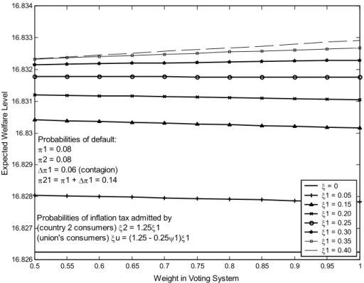
by the high-weight country, its welfare is affected by opposite choices.

3.6.1 Welfare for member country with high weight in voting system

• Dollar debt in the no-crisis zone for s1

= (kn_{, B}1

, D, 1, 1,·,·, ·, ·)

For dollar debt levels in the no-crisis zone, external creditors know that the

national government always prefers to pay back its debts, no matter what the

realization of the sunspot variables is. The expected welfare for country 1is

Vn³s1´

1

1−β

n

vhθyn₋(1₋β)B1

−(1₋β)Di+%[(1₋θ)yn+ (1₋β)D]o

• Dollar debt in the crisis zone for s1

= (kπξu

, B1

, D, 1,1, ζ1 , ζ2

, η1 , ·)

When dollar debt is in the crisis zone, the realization of the sunspot variables

has bearing. Given and the expected welfare is

Vπξu³s1´

= (1−π)Vπξu³s1

, B01

, q∗πξu, D, qπξu´+ (16)

h ππ21

(si+asi) +π(1₋π21

)ξ1i

Vπφ³s1

, B01

,β(1₋π), D,βφ´+ h

ππ21

(sni+asni) +π(1₋π21

)³1₋ξ1´i

Vd³s1

,0,0, D,β´

where, Vπξu

(s1 ,B01

,q∗πξu

,D,qπξu

) is the expected welfare with positive probability

that country 1 defaults on dollar debt or that an inflation tax is created in the

following period,Vπφ_(s1 ,B01

,β(1₋π),D,βφ) is the expected welfare after inflation

tax on common-currency debt and possibility of a moratorium on dollar debt next

period, and Vd_(s1

,0,0, D,β), after country 1 defaults.

3.6.2 Welfare for member country with low weight in voting system

• Dollar debt in the no-crisis zone for s2

= (kπξ1

, B2

, D, 1,1, ζ1 , ·,η1

, ·)

The expected welfare depends on sunspots from country 1and is equal to

Vπξ1³s2´

= (1₋π) Vπξ1³s2

, B02

,β, D, qπξ1´+ (17)

π asi0 Vπφ³s2

, B02

,β, D,βφ´+π si0 Vd³s2

, B02

,β, D,β´

where Vπξ1

(s2

, B02

, β, D, qπξ1

) is the expected welfare when sunspots for country 1

indicates possible default on dollar debt or inflation in the following period,Vπφ_(s2

,

B02

,β, D,βφ) is the expected welfare if the central government creates inflation tax,

and Vd_(s2

, B02

, β, D, β) is the payoff when country 1 defaults. As long as dollar

debt for country 2 belongs to the no-crisis zone and country 1 has defaulted, then

• Dollar debt in the crisis zone for s2

= (kπξu

, B2

, D, 1,1, ζ1, ζ2, η1 , η2

)

Vππ2ξu³s2´

= (18)

(1₋π)³1₋π2´

Vππ2ξu³s2

, B02

, q∗ππ2ξu, D, qπξu´+ h

ππ21

(si+asi) +π³1₋π21´

ξ1i

Vππ21φ³s2

, B02

, q∗ππ21φ, D,βφ´

π³1−π21´ ³

1−ξ1´ Vπ2³s2

, B02

,β³1−π2´

, D,β´+ h

ππ21

(sni+asni) + (1−π)π2i

Vd³s2

,0,0, D,β´

where Vππ2_ξu

(s2 ,B02

,q∗ππ2_ξu

,D, qπξu

) is the expected welfare when there is positive

probability of default in both countries or inflation tax on common-currency debt

next period, Vππ21_φ

(s2 , B02

, q∗ππ21_φ

, D, βφ), when the central government has

created inflation tax, but both countries may still default on their dollar debts

in the following period, Vπ2

(s2 ,B02

,β(1₋π2

), D,β), when country 1defaults and

there is positive probability that country2will default in the future, andVd_(s2

, B02

,

β, D, β), after country2 defaults.

3.6.3 Welfare when central bank is under political pressure

As with common currency, local currency is used with the subterfuge that the

monetary authorities have some control over monetary policy. In contrast, to the

central bank of a monetary union whose decisions considers all member countries,

we assume that the central bank from a country that issues its own local currency

may be subject to political influence of its government not so strongly committed

with fiscal discipline. Given the ability to inflate local currency, the private sector

anticipates that the central bank may create an inflation tax despite the abscence

of an external debt crisis.

The dependence of the central bank on the political decision of its government

is captured by the probability ψξ that the central bank will inflate even though

the external creditors renew their loans. We assume that, before the realization of

will not inflate the local-currency debt, given that the bankers’ confidence in the

government is high, is ψξ, i.e P[η _≤ ξ | ζ > π] = ψξ. When ψ equals zero, the

central bank is independent (denoted as strong) and resorts to inflation only to avoid

an external debt crisis, as we assume throughout the model with common-currency.

When ψ is positive, the private sector attributes probability ψξ that the central

bank is dependent (called weak) and practices a monetary policy influenced by the

government. Political pressure is absent in the original Cole-Kehoe model.

4

A Numerical Exercise

We carry out simulations for the Brazilian economy, as if Brazil were a member of

a monetary union with two member countries. We consider two situations: one in

which it has high weight in the voting system (ϕ1

>0.5) and the other, low weight

(ϕ1

≤0.5).

4.1

Parameters for the Brazilian Economy

The parameters refer to the Brazilian economy from June 1999 to May 2001.

The 24-months interval matches the average maturity of the Brazilian government

domestic debt, in particular, of bonds indexed by the Selic rate and by the dollar.

The other parameters used in the simulations are: production function f(k)

= Akν _{with capital share, ν = 0.5 and total factor productivity, A = 0.8; tax}

rate, θ = 0.3; utility function of public goods, v(g) = (1/10) log(g) + 1; weight of

utility of private relative to public consumption, %= 0.7; drop in productivity after

default, α = 0.95; discount factor, β = 0.93; depreciation factor, δ = 0.20; total

common-currency debt relative to gross domestic product, D/GDP = 0.3.

In the original numerical exercise for Mexico, v is a logarithmic function, ln(g).

With this specification, Cole and Kehoe obtained positive values for this utility,

whereas our simulations for Brazil produce only negative values for all levels of

the dollar debt. Therefore, we changed v(g) to (1/10) log(g) + 1 to overcome this

of private consumption,c, in consumer utility, we reduced the parameter%from one

to 0.7.

Public Sector Debt

According to our model, D is the government debt that may be inflated away

in case of an external debt crisis. In the numerical exercises, it is parameterized

as the internal net public sector debt denominated in Brazilian money. To

exclude dollar-indexed debt, we assume that the fraction of dollar-indexed bonds

in the internal net public sector debt is the same as its share in the amount

of federal government bonds outside central bank. In this way, we obtain that

common-currency debt, D, relative to GDP is approximately equal to 0.30 for the

period under analysis (Araujo and Leon [2], Tabela 3).

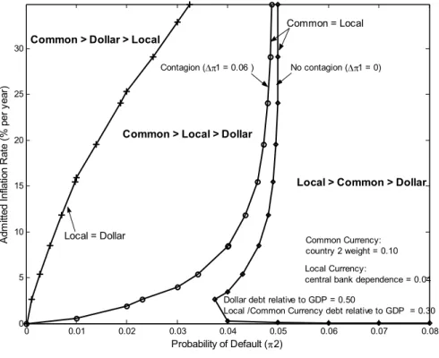
On the other hand, the model definesB as the government debt that may suffer

a speculative attack, if its level is in the crisis zone. In Araujo and Leon ([2], Tabela

3), B is described as the Brazilian public sector debt denominated in dollar and

equivalent to the sum of external public sector debt (less international reserves) and

internal net public sector debt indexed to the dollar. For the period under analysis,

its average value is 0.20 relative to GDP. According to the results of the present

paper, at this level,B is below the crisis zone, since the lower limit of the crisis zone

is obtained around 0.38 relative to GDP. However, it would be more reasonable if

the Brazilian public sector debt denominated in dollar were in the crisis zone and

this is the exercise that we do using our model.

In the numerical exercises, we make the strong hypothesis that the Brazilian

public sector dollar debt relative to GDP is 0.50. This number refers to the sum of

internal net public sector debt indexed to the dollar and total external debt (private

plus public, not just public). This assumption finds some ground on the practice of

sovereign credit rating agencies. After the Asian crisis, they became more concerned

about implicit government support of private sector claims (Bhatia [5], p. 23). In

the simulations, total external debt refers to annual gross external debt (excluding

216.9, for 2000, and 209.9, for 2001; Brazilian GDP, in billion dollars, is 590.7, for

2000, and 541.9, for the following year; and finally, external debt relative to GDP

is 0.37 and 0.39, respectively. Furthermore, in Araujo and Leon ([2], Tabela 3),

public sector debt indexed to the dollar is obtained around 0.10 relative to GDP,

on average, from June 1999 to May 2001. Therefore, using our strong hypothesis,

public sector dollar debt relative to GDP is close to 0.50.

Since common-curency debt, D, is fixed at 0.30 relative to GDP, then public

sector debt (common plus dollar denominated) is equal to0.80. Such high magnitude

for the Brazilian public sector debt is more in conformity with estimations from

credit rating agencies than with official figures, but our main objective so far

is to develop a procedure to analyse public sector debt subject to a speculative

attack. Additional research on the specification of the utility functions could possibly

produce a more reasonable crisis zone than the one we obtained in our numerical

exercise and in this way avoid the hypothesis of government responsability for private

sector external debt. This is a suggestion for future studies.

Abatement Factor,φ

The abatement factor, φ, is supposed to be a function of the probability that

government i votes for inflation tax, ξi, in the following way. By analogy with π,

ξi is defined as the ratio between the tax rate for bonds denominated in common currency, ii_{, and bonds denominated in dollars, r}i_{, both issued by country i, given}

by

ξi = 1₋ Ã

1 +ii

1 +ri

!

According to the uncovered interest parity, 1/(1₋ξi) is equal to one plus the rate of devaluation of the common currency relative to the dollar that consumers from

countryi expect. Assumingξi is small, then we can approximateξi as the expected rate of devaluation of the common currency in country i. The expected rate of

devaluation of the common currency by all consumers from the union is defined as

ξu =ϕ1

ξ1

+³1₋ϕ1´

where ϕ1

is the weight of country 1 in the voting system. We make the hypothesis

that one plus the expected rate of devaluation of the common currency and one plus

the expected rate of inflation are equal and, by rational expectations, the expected

rate of inflation actually occurs. Therefore, we have

1/(1−ξu) = 1 +χe= 1 +χ= 1

φ (19)

or

1−φ=ξu

As we can see, the inflation tax on common curency debt, (1₋φ), is equal to the

rate of devaluation of the common currency, ξu, which in turn depends only on the expected rate of devaluation in each country and the weight of country1in the voting

system. To simplify the numerical exercises, we assume two cases (ξ2 = 0.75ξ1 and

ξ2

= 1.25 ξ1

) and make a grid of values for ξ1

≤ 0.5. Another parameter used in the simulations to represent the abatement of the real return on common-currency

debt is φn, for the case of ξ2

being equal to zero.

Inflation Cost

Another parameter to be considered isαφ_{, the productivity of the economy after}

inflation. Simonsen and Cysne ([9], p.14) calculate the cost of inflation in Brazil as

a fraction of GDP for a given inflation rate. Their equation is

F(χ_l) = 1.105 log(1 + 0.0368χ0.475

l ) (20)

where F(χ_l) is the inflation cost relative to GDP and χ_l is the annual periodic inflation rate in logarithmic form. χ_l is related to the parameter φ (of the common-currency model) by expression χ_l = log(1/φ). To computeαφ _{for different}

values of φ, we compare the cost of inflation given by expression (20) to the welfare

loss after inflation in the Cole-Kehoe model. To simplify the calculations, we suppose

that dollar debt is stationary at b(kn_{, D). Therefore, for given φ, we have the}

following equation with αφ _unknown

F(φ) = u

φ_(s1

)₋un_(s1

)

where un_(s1

)and uφ_(s1

) are one-period utility without and with inflation, specified

as

uφ(s1) =vhθynφ−(1−β)b(kn, D)−φ(1−β)Di+%h(1−θ)ynφ+φ(1−β)Di

un(s1

) =vhθyn₋(1₋β)b(kn, D)₋(1₋β)Di+%[(1₋θ)yn+ (1₋β)D]

with s1

= (kn_{, b(k}n_{, D), D, 1, 1, ·, ·, ·, ·) and y}nφ _=αφ_A(kn₎γ

−δkn_{. We assume}

unappropriately that the consumer’s investiment after inflation is kn_{instead of k}nφ_.

Nevertheless, the difference between them is small numerically. A similar procedure

is applied to obtain αφn

, in whichφn substitutes for φ.

Correlation between ζ1 and ζ2

The parameter πi _{is the probability that country i defaults, given that other}

countries with strong comercial andfinancial ties with it are not under a speculative

attack. When we assume that Brazil has more than 50 percent weight in the voting

system, the probability of default for country1,π, is estimated as the average EMBI+

sovereign spread calculated by J. P. Morgan. A crisis that affects international

bankers’ confidence in Brazil also influences another country that is integrated to it,

like Argentina. Therefore, when Brazil is country 1, we consider Argentina country

2. Accordingly, π2

is the sovereign spread for Argentina when Brazil is not under a

speculative attack and π21

, when it is. We defineπ21 as

π21

=π2

+∆π2

(21)

and ∆π2

is the change in sovereign spread of country 2 when country 1 is under a

speculative attack on its dollar debt.

Following the procedure of Hernández and Valdés [11] in a simpler way, a linear

regression model is used to represent the relation between the changes in sovereign

spreads of the two countries, ∆π1

and ∆π2

, when country 1 is under an external

debt crisis