NEW VOLATILITY MODELS UNDER A BAYESIAN
PERSPECTIVE: A CASE STUDY
Edilberto Cepeda Cuervo*
Jorge Alberto Achcar† Milton Barossi-Filho‡
Abstract
In this paper, we present a brief description of ARCH, GARCH and EGARCH models. Usually, their parameter estimates are obtained us-ing maximum likelihood methods. Considerus-ing new methodological pro-cesses to model the volatilities of time series, we need to use other infer-ence approach to get estimates for the parameters of the models, since we can encouter great difficulties in obtaining the maximum likelihood
es-timates due to the complexity of the likelihood function. In this way, we obtain the inferences for the volatilities of time series under a Bayesian ap-proach, especially using popular simulation algorithms such as the Markov Chain Monte Carlo (MCMC) methods. As an application to illustrate the proposed methodology, we analyze a financial time series of the Gillette Company ranging from January, 1999 to May, 2003.
Keywords: ARCH; GARCH; EGARCH; Stochastic Volatility Models; Fi-nancial Time Series; Bayesian methodology; MCMC methods.
Resumo
Neste artigo, apresentamos uma breve descrição dos modelos ARCH, GARCH e EGARCH. Normalmente, as estimativas dos parâmetros des-ses modelos são obtidos através de métodos de máxima verossimilhança. Considerando-se novos processos metodológicos para modelar as volatili-dades das séries temporais, precisamos usar outra abordagem de inferên-cia para obter estimativas para os parâmetros dos modelos, uma vez que podemos ter grandes dificuldades para obter as estimativas de máxima verossimilhança, devido à complexidade da função de verossimilhança. Desta forma, obtemos as inferências para as volatilidades das séries tem-porais sob uma abordagem bayesiana, especialmente com o uso de algorit-mos populares de simulação como o método de Monte Carlo em Cadeias de Markov (MCCM). Como uma aplicação para ilustrar a metodologia pro-posta, analisamos uma série temporal financeira da empresa Gillette vari-ando de janeiro de 1999 à maio de 2003.
Palavras-chave:ARCH; GARCH; EGARCH; Modelos de Volatilidade Es-tocástica; Series de tempo Financieras; Métodos Bayesianos; Métodos de MCMC.
JEL classification:C53
DOI:http://dx.doi.org/10.1590/1413-8050/ea91
*Universidad Nacional de Colombia. Departamento de Estatística. E-mail: [email protected] †Universidade de São Paulo, FMRP, Brazil. Departamento de Medicina Social. E-mail:
‡Universidade de São Paulo, Brazil. Faculdade de Economia, Administração e Contabilidade de
Ribeirão Preto. E-mail: [email protected]
1
Introduction
Financial time series volatility has been an issue that academics have focused on since Engle (1982) seminal paper. Mostly, volatility appeared to be an im-portant issue after the abandonment of fixed parities dollar-gold by the USA at the beginning of the 70’s. Since then, asset prices started changing more broadly, especially international exchange rates. After exchange raa’ markets’ volatility rising, it was just a matter of time for verifying the same in stock mar-kets, mainly in the 80’s and 90’s. In order to frame this new phenomenon into feasible financial models, researchers kept on looking for alternative method-ologies which reproduces excess volatility; a new stylized fact showed by fi-nancial time series.
Engle (1982) and Bollerslev (1986) offered a primary sort of answer to this
issue, the so called ARCH class models. Intrinsically those models are lep-tokurtic and are, for instance able to capture the excess volatility contained in most financial time series. However this was not the first concern of Engle, whose applicative example take the UK inflation rates time series into account. Extending this empirical practice to other time series, mainly financial, was the next step.
After obtaining success on incorporating excess volatility into ARCH class models, another stylized fact arises from empirical data. Repeatedly, aca-demics and financial analysts verified that financial volatility produced a skew impact on asset prices; i.e. bad news tends to impact more severely on asset prices than good news. In order to incorporate this stylized fact into volatility models, Nelson (1991) proposed an EGARCH class of models.
Though all these models recognized volatility is a latent variable, a more satisfactory answer to the problem of adjusting volatility as a stochastic model was provided by the stochastic volatility models. Hull & White (1987) is a reference on this matter by adjusting a stochastic volatility process into op-tion pricing formulas and, obtaining better results than the original Black & Scholes (1973) option pricing model. In fact stochastic volatility models are a more flexible alternative for modeling financial time series, once one stochastic process is assumed for the random terms. However, these stochas-tic processes are still normal, guarantying a closed solution for the likelihood function.
From a methodological point of view Bayesian models are a generalization of those models briefly discussed above. Bayesian methods are more suitable for modeling financial time series and forecasting their future behavior as well, because they allow for an introduction of a broad variety of stochastic processes for describing latent variables; i.e. prior distributions. Definitely, classic inference dominates financial literature on modeling and forecasting time series behavior, however Bayesian inference is becoming a better alterna-tive for the same reason, mainly after the rapid computational development in the 90s. Moreover, once Bayesian approach provides a broad way for mod-eling the stochastic term, better results can be obtained for estimating and forecasting financial time series behavior.
Compar-ative studies between SV models and models type GARCH are well known in the literature (see for example, Taylor 1994, Ghysels et al. 1996, Shephard 1996, Kim et al. 1998).
Bayesian Methods using Markov Chain Monte Carlo (MCMC) methods are considered in the analysis of financial time series assuming SV models (see for example, Meyer & Yu 2000), given the great difficulties in the classical
statistical approach with the complexity of the likelihood function.
This article is divided into 5 sections. In section 2 we define the ARCH in regression models proposed by Engle (1982), the generalized ARCH models or GARCH, introduced by Bollerslev (1986) and the exponential GARCH models or EGARCH, proposed by Nelson (1991). In section 3, we propose a Bayesian methodology to fit general exponential autoregressive models, GEGARCH. In section 4, generalized stochastic volatility models or GSV, are defined. In sec-tion 5, we introduce a Bayesian analysis for GSV models. In secsec-tion 6, the time series of prices and log-returns of the shares prices for the Gillette Com-pany are analyzed, assuming different models for both time series. Finally,
in section 7, we present some conclusions. The selection of the best model is made using the AIC (Akaike Information Criterion) and BIC (Bayes Informa-tion Criterion).
Finally, in section 7, we present some conclusions.
2
ARCH, GARCH and EGARCH models
2.1 ARCH models
If a random variable yt is drawn from the conditional density functionf(yt| ψt−1), the forecast of today’s value based on the past informationψt−1is given
byµt=E(yt|ψt−1) and can be modeled as a regression modelµt=x′tβ, where xt=
1, xt1, . . . , xtq ′
is the vector of the explanatory variables at timet, for
ex-amplext=
1, yt−1, . . . , yt−q ′
, andβ=β0, β1, . . . , βq ′
is the vector of regression mean parameters. At this time we also suppose that the conditional vari-ance V(yt|ψt−1), depends on the past information through the model ht = hα0+α1ǫ2t−1+. . .+αpǫ2t−p
whereα =α0, α1, . . . , αp ′
is the vector of condi-tional variance parameters,ǫt=yt−1−x′tβ andhis a real monotone function that takes into account the positivity of the variance.
Thus, the stochastic process{yt}t∈I follows a p-order linear ARCH model or ARCH(p) (Engle 1983) that can be rewritten by:
yt|ψt−1∼N(µt, ht) (1)
µt=x′tβ (2)
ht=z′tw=α0+α1ǫt2−1+. . .+αpǫ2t−p
ǫt=yt−1−x′tβ
wherew′=α0, α1, . . . , αp
andzt′=1, ǫ2t−1, ǫ2t−2, . . . , ǫt2−p.
model and from the squared residuals (Tsay 2002). Another way is to use a Lagrange multipliers LM test, proposed by Engle (1982) and Bollerslev (1986) in which, after expressinghtasht=z′t1ω1andht=z′t1ω1+z′t2ω2, we will test
the null hypothesisH0:ω2= 0. By accepting this hypothesis we demonstrate
the dimension of the ARCH effect is not more than the dimension ofω1.
2.2 GARCH Models
Let {yt}t∈I be a stochastic process, where I is a discrete process, as given in section 2.1. In the GARCH(p, q) regression model the mean model is defined by (2), but the conditional variance models also depends on the conditional variances, as shown by the next equation
ht=z′tω=α0+
p X
i=1
αiǫ2t−i+ q X
i=1
γiht−i (3)
wherep≥0,q >0,αi≥0,γi≥0,i= 1, . . . , p. In this equationsω′= (α0, α1, . . . , αq, γ1, . . . , γp) andzt=
1, ǫt2−1, . . . , ǫ2t−q, ht−1, . . . , ht−p
are the vectors of the vari-ance parameters and the varivari-ance explanatory variables, respectively. Ifq= 0, we have an ARCH(p) regression process.
Usually, GARCH models do not fully reflect the nature of the volatility of most financial assets. These models do not take into account asymmetri-cal behavior typiasymmetri-cal of the price volatility of financial assets, which is a well-known leverage effect. In GARCH models, the conditional volatility of the
as-set prices is affected symmetrically by positive or negative innovations. In
ad-dition, the parameters in the volatility model are restricted to non-negativity. Evidences of this effect have been found by Nelson (1991), Glosten et al. (1993)
and Engle & Ng (1993), among many others.
2.3 EGARCH Models
Including the asymmetrical effect given by the fluctuations in the volatility of
the asset prices, Nelson (1991) proposed the Exponential class GARCH mod-els, or EGARCH(p,q) models. In this class of modmod-els, the conditional variance equation is defined in terms of the standard normal variatezt=ǫt/σtand the unexpected log-return through the equation,
logσt2
=α0+
p X
i=1
αi(|zt−i|+λizt−i) + q X
j=1 βjlog
σt2−j
whereθ=α1, . . . , αp, β1, . . . , βq
is de vector of parameters. In this model, the effect of asymmetry is considered. Bad news can have a large impact on the
volatility, and the values ofλiwould expected to be negative.
Several studies have found that EGARCH models fit financial data very well, much better than the other GARCH models. The advantages of the ponential specification for the variance are given by many others (see, for ex-ample, Taylor 1994, Heynen et al. 1994, Lumsdaine 1995).
3
A General EGARCH Model: a Bayesian approach
Similar to Engle (1982), the {yt}t∈I process follows the autoregressive condi-tional heteroscedastic model if,
yt|ψt−1∼N(µt, ht) (4)
µt=x′tβ
ht=exp
α0+α1z1,t+. . .+αpzp,t
where, for example,zi,t=ǫt−i, zi,t=ǫ2t−i, zi,t=ǫhtt−i
−i, zi,t=ht−i, andǫt=yt−x
′
tβ. The explanatory variables of the volatility model can also include terms of some other financial time series. As in section 2.1, in this model, β is the vector of mean parameters,xtis the vector of the mean explanatory variables andα′=α0, α1, . . . , αp
is the vector of volatility parameters.
Assuming a general EGARCH model, we could have difficulties in
obtain-ing maximum likelihood estimates for the parameters of the model. A suitable alternative is to use Bayesian methods.
In order to estimate the parameters under the Bayesian methodology, we need a prior distribution for the parameters assessing the information about what we would anticipate as the relative frequency from a very large num-ber of observations. For simplicity, we assign the prior distributionp(β, α)∼
N(θ0,Σ0), where θ′0 = (b, g) and Σ0 is a (q+p)×(q+p) variance covariance
matrix forθ= (β, α). Then, with the likelihoodL(β, α) given by some distri-bution that belongs to the two parameter exponential family, and using Bayes theorem, we find the posterior distribution π(β, γ) ∼L(β, α)p(β, α). Given that π(β, α) is analytically intractable and not easily generated, we propose sampling (β, α)′ in an iterative process; i.e. samplingβfrom a q-dimensional random walk andαfromπ(α|β) distribution.
Consequently, ifβ(c) andα(c) are the current values ofβ and α, the new
values ofβ=β0, β1, β2, . . . , βq ′
are proposed as a multivariate random walk. New values ofαare obtained as it is proposed by Cepeda & Gamerman (2001) from
q2
α|α,ˆ βˆ=N(g∗, G∗) (5)
whereg∗ =G∗G−1g+12Z′Y˜, G∗ =G−1+12Z′Z−1,b andGare given by the conditional prior distributionγ|β∼N(g, G), andZis the matrix with t-th row equal to1, z1,t, . . . , zp,t
and ˜Y is the n-dimensional vector with the i-th com-ponent equal to ˜yi = yiσ−iµi −1. This proposal is obtained from Fisher scoring.
We also could obtain the working variables by Taylor approximation. In this case the working variable is ˜yi=yiσ−iµi.
4
Stochastic Volatility Models
yt=σtǫt, t= 1,2, . . . , n (6)
whereǫt is a sequence of i.i.d. random variables with normal distribution N0, σǫ2
. In this model, the volatility of the time series yt is given by the conditional varianceσt2=E
yt2|Ht
, whereHt={yt−1, yt−2. . .}are the observed
values at timest−1, t−2, . . .. Here we assume that the standard deviation is given by the model,
σt=exp (
ht 2 )
(7)
wherehtis a latent variable defined by the autoregressive model
ht=µ+φ(ht−1−µ) +ηt t= 2,3, . . . (8)
and we assume that h1 is a random variable with known distributionP1(h1)
andηtis a sequence of i.i.d. random variables with normal distributionN(0, ση2). If|φ|<1 the mean and the non-conditional variance ofht areE(ht) =µ
andV ar(ht) = σ2
η
(1+φρ1), whereρ1is the coe
fficient of autocorrelation between
htandht−1(see for example, Taylor 1994).
With the assumptions (5), (6) and (7), we have
yt∼N
0, σε2exp{ht}
(9)
h1∼N
µ, ση2
(10)
ht|ht−1∼N
µ+φ(ht−1−µ), ση2
(11)
fort= 2,3, . . . n.
A generalization of the stochastic volatility model, given by (5) and (6), can be obtained by defining a model through (11) for the latent variable defined by
ht=µ+ p X
j=1 φj
ht−j−µ
+ηt (12)
fort=p+ 1, . . . , n, with roots of polynomialφ(B) = 1−Pp
j=1φjBj outside the unit circle (B is the retarded operator defined by Bqht = ht−q). The model defined by (5) and (6) and (11) is called Generalized Stochastically Volatility model (GSV).
In this case,
ht|ht−1, . . . , ht−p∼N
µ+ p X
j=1 φj
ht−j−µ
, ση2
(13)
fort= 2,3, . . . , n.
L= n Y
t=1
p(yt|ht) (14)
From (8), we obtain:
L= n Y t=1 1 q
2πσǫ2exp{ht} exp
(
− y
2
t 2σǫ2exp{ht}
)
(15)
With this new generalized stochastic Volatility Model, we can obtain better inferences for the volatilities of financial time series.
5
Bayesian analysis of GSV model
For a Bayesian analysis of the Stochastic volatility model defined by (5) and (6), with latent variables defined by (11), we assume the following prior dis-tributions forµ,Φ=φ1, φ2, . . . , φp′,σ2
ǫ andση2.
φj∼B
aj, bj
, j= 1, . . . , p (16)
σǫ2∼IG(c1, d1) (17)
ση2∼IG(c2, d2) (18)
µ∼N0, e2 (19)
where Baj, bj
denotes a beta distribution with mean (aaj
j+bj) and variance
ajbj
(aj+bj)2(aj+bj+1)
;IG(c, d) denotes the inverse gamma distribution with mean
d
(c−1) and variance
d2 h
(c−1)2(c−2)i, c >2, andN
µ, σ2denotes the normal
distri-bution with mean µ and varianceσ2. We assume that the hyperparameters
aj, bj
, j= 1, . . . , p,(ci, di), i= 1,2, ande2are known.
Ifhl = 0, forl= 0,−1, . . . ,−p+ 1 in (12), the conditional distribution ofht givenh(tp−)1={ht−1, . . . ht−p}, fort= 1, . . . , n, is given by
p
ht|h
(p)
t−1
=q 1 2πση2
exp − 1
2ση2
ht−µ− p X
j=1 φj
ht−j−µ
2 (20)
Thus, ifΦ=φ1. . . , φp′, θ=µ,Φ, σǫ2, ση2, h= (h1, . . . , hn)′and ifµ,Φ, σǫ2, ση2
π(ϕ|y) = n Y t=1 1 q
2πσǫ2exp{ht} exp
(
− y
2
t 2πσǫ2exp{ht}
)
×p 1
2πσǫ2 exp − 1
2ση2
ht−µ− p X
j=1 φj
ht−j−µ
2
π(θ)
wherey= (y1, . . . , yn)′andπ(θ) is given by
π(θ)∝
p Y j=1
φajj−11−φj bj−1
ση2 −(c1+1)2
exp
−d1
ση2
×σǫ2 −(c2+1)2
exp
−d2
ση2 exp ( −µ 2
2e2 )
Thus, the posterior density can be rewritten as
π(ϕ|y)∝σǫ2 −n2
exp −1 2 n X t=1 ht−
1 2σǫ2
n X
t=1
yt2exp{−ht}
×ση2 −n2
exp − 1
2ση2 n X t=1
ht−µ− p X
j=1 φj
ht−j−µ
2
π(θ)
(21)
Finally, ifΦ=φ1. . . , φp′, y=y2
1, . . . , yn2
, h= (hi, . . . , hn)′, E(h) =
e−hi, . . . , e−hN′
and the matrixXgiven by:
X=
h0 h−1 . . . h−p+1 h1 h0 . . . h−p+2
..
. ... . . . ... hp hp−1 . . . h1 hp+1 hp . . . h2
..
. ... . . . ... hn−1 hn−2 . . . hn−p
n×p ,
the posterior density (20) can be written as
π(ϕ|y)∝σǫ2 −n2
exp (
−121′h− 1
2σǫ2 y′E(h)
)
×ση2 −n2
exp − 1
2ση2
(h−µ−X′Φ)′(h−µ−X′Φ)
π(θ)
Sampling from the joint posterior distribution ofϕ(θ, h), we use MCMC methods with Gibbs Sampling algorithm (Gelfand & Smith 1990) or Metropolis-Hastings (Smith & Roberts 1993). These samples are generated from the con-ditional distributionsφθj|θ(j), y
, whereθ(j)denotes the vector of all
compo-nents ofθ, except thej−thcomponent.
6
An Application
As an application, we analyze the time series of prices and log-returns of share prices of the Gillette Company, taken daily at the closing of the market, from January, 1999 to May, 2003. The results were obtained using the statistical program Eviews 5.0, for ARCH, GARCH and EGARCH models under the clas-sical inference approach, and WinBugs software (Spiegelhalter et al. 1999) under Bayesian inference approach. Moreover, the selection procedure was based on the AIC (Akaike Information Criterion) and BIC (Bayes Information Criterion). In all cases, the Q statistics of Ljung-Box do not reject the nullhy-pothesis1
BIC (Bayes Information Criterion) is a model discrimination criterion in-troduced by Schwarz (1978) and modified by Carlin & Louis (2000) to be ap-plied assuming the posterior density for the parameters of the fitted model. This criterion weights between the maximized likelihood function and the number of parameters of the model. The best model is the one with larger value of BIC.
6.1 Models for shares’ prices
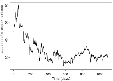
In order to illustrate the results provided by the models discussed in this pa-per we took Gillette’s stock prices time series on a daily basis at the closing market index lasting from January, 1999 to May, 2003. Figure 1 shows the behavior of this time series and what strikes us most is a general descending feature of these prices. This behavior is surely explained by the microeco-nomic aspects of this Company, once this used to be a typical period of stock market boom.
Observing the pattern showed in Figure 1, it is quite precise to state that there are four price cycles lasting one year each. Probably, as a stylized fact, this finding is linked to the product’s life cycle released to the market on an annual basis. Gillette is an internationally well-known brand of men’s safety razors, amongst other personal care products and it used to be a leading global supplier of these products until it merged with Procter & Gamble in 2005. It appears to be the Company’s strategies on releasing new products followed a life cycle as expected, but these strategies were also accompanied by a steady decrease in the Company’s market value.
After taking a closer look at Gillette’s history since the 70’s, we can see that this Company went through takeover attempts more than once and faced judicial dispute claims for its products prior to merging with P&G in 2005.
From the macroeconomic point of view Gillette’s stock prices diverged from the expected behavior of stock market prices in this time period. Stock
1H: there is no serial correlation for residuals, as for square residuals., at a 1% significance
prices data for Gillette covers roughly the second term of Clinton’s adminis-tration in USA, a period of economic and financial boom. In recent times this period demonstrated one of the most economic and financial growing virtu-ous cycle, contrasting with the poor performance of Gillette’s stock prices.
Besides these incidents in corporate management, Gillette also faced the fact that it used to be a traditional Company clearly affected by issues such
as technology decline, more efficient competitors, amongst others. Definitely,
Gillette did not introduce itself into the technological development stream that characterized the time period analyzed. After merging with Procter & Gamble in 2005, Gillette faced its dissolution and was finally incorporated as a division of P&G in 2007.
0 200 400 600 800 1000
30
40
50
60
Gillette’s stock prices
Time (days)
Figure 1: Time series of the prices.
ARCH Models
Among different ARCH models, the ARCH(4) model has the smallest BIC
value. The maximum likelihood estimates (MLE) of the mean and variance parameters, and their standard deviations, are given in Table 1.
Table 1: Maximum likelihood parameter estimates of ARCH(4) model.
Parameter β0 β1 α0 α1 α2 α3 α4
Mean −0.1350 1.005 0.2195 0.4652 0.0826 0.2009 0.0892 s. d. 0.0610 0.001 0.0199 0.0398 0.0277 0.0306 0.0179
The p-values associated with the tests H :θ = 0 versus θ , 0, whereθ
0.004, except the p-value associated withβ0, that is given by 0.027. The AIC
and BIC values are given by 2.2201 and 2.2524, respectively.
GARCH Models
Among different GARCH models, the GARCH(1, 2) model has the smallest
BIC value. The MLE estimates of the mean and variance parameters, and their standard deviations are given in Table 2.
Table 2: Maximum likelihood parameter estimates of GARCH(1,2) model.
Parameter β0 β1 α0 α1 α2 γ1
Mean 0.4566 0.9857 0.2195 0.4656 0.0826 0.2009 s. d. 0.1583 0.0044 0.0199 0.0398 0.0277 0.0306
The p-values associated with the test H:θ= 0 versusθ,0, whereθ
repre-sents all regression parameters, are all smaller than 0.006. The AIC and BIC values are given by 2.1059 and 2.1336, respectively.
General EGARCH Models
In this section, we fit two models to analyze the time series of prices and log-returns of Shares of the Gillette Company, applying the Bayesian methodology given in section 3. In both models, yt|ψt−1∼N(µt, ht) withµt=β0+β1yt−1,
whereβ′= (β0, β1) is the mean parameter vector.
We assume normal prior distribution,N0,10k, for all parameters with large variances,k= 5 to have approximately non informative priors, consider-ing two different models for the prices.
Model 1. Here we assume that the conditional variance of the stochastic processYt,t∈T is given by the model
ht= exp
α0+α1ǫt2−1+α2ǫt−2
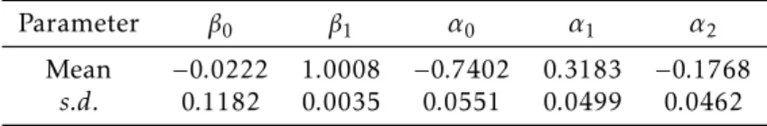
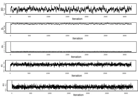
whereα′ = (α0, α1, α2) is the vector of variance parameters andǫt=yt−x′tβ. The parameter estimates (posterior means) of this model are given in Table 3. Figure 2 shows the behavior of the chain sample for each parameter, each one of which has a small transient stage, indicating the speed convergence of the algorithm. The chain samples are given for the first 4500 iterations. The other results reported in this section are based on a sample of 4000 draws after a burn-in of 1000 draws.
Table 3: Posterior summaries for the prices model (model 1)
Parameter β0 β1 α0 α1 α2
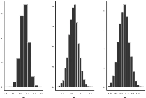
The histograms of the generated samples for each parameter seem to show that the posterior marginal distribution for all the parameters is approxi-mately normal. Figure 3 shows the histograms for the posterior marginal distributions of the variance parameters.
According to a theoretical result in which the model where the information matrix is not block diagonal, Table 4 shows a large correlation between mean and variance parameters. For this model the AIC and BIC values are given by 2.330 and 2.3228, respectively.
Table 4: Posterior summaries for the correlation between the parameters (model 1)
Parameters β0 β1 α0 α1 α2
β0 1
β1 −0.976 1
α0 0.121 −0.156 1
α1 −0.196 0.230 −0.633 1 α2 0.156 −0.141 0.178 −0.234 1
0 500 1000 1500 2000 2500 3000
Iteration
-0.4
0.0
0.4
β
0
0 500 1000 1500 2000 2500 3000
Iteration
0.90
0.96
β
1
0 500 1000 1500 2000 2500 3000
Iteration
-1
0
1
2
3
4
α
0
0 500 1000 1500 2000 2500 3000
Iteration
0.0
0.2
0.4
α
1
0 500 1000 1500 2000 2500 3000
Iteration
-0.3
-0.1
α
2
Figure 2: Time series plots for the simulated sample for each parameter
Model 2. Here we assume that the conditional variance of the stochastic processYt,t∈I is given by the model,
ht= exp
α0+α1ǫt2−1+α2ǫ2t−2
-1.0 -0.9 -0.8 -0.7 -0.6 -0.5
0
2
4
6
α0
0.2 0.3 0.4 0.5
0
2
4
6
8
α1
-0.30 -0.25 -0.20 -0.15 -0.10 -0.05
0
2
4
6
8
α2
Figure 3: Marginal posterior distribution for the variance parameters
The posterior samples were recorded every 10th sample, after a burn-in period of 1,000 Gibbs samples, to have approximately uncorrelated samples. The posterior summaries for this model are given in Table 5.
Table 5: Posterior summaries for the prices model (model 2)
Parameter β0 β1 α0 α1 α2
Mean 0.0473 0.9989 −0.7217 0.2714 0.0395 s. d. 0.1327 0.0040 0.0553 0.0533 0.0229
In this case, each one of the chain shows small transient stage, indicating the speed convergence of the algorithm. The histograms for the generated samples for the parameters also show that the posterior marginal distribu-tions for all the parameters are approximately normal, and the correlation between posterior parameter sampling shows that 0.11 <corr(βi, αj)<0.31, that is, a small value, but all significatively different from zero. The AIC and
BIC values for this model are given by 2.3198 and 2.3234, respectively. From the obtained results for all assumed models, we observed that model 1 is a best model fit for time series of prices for Gillette, since the BIC value associated with this model is the smallest when compared to the other models.
6.2 Models for the log-return Gillette series
LetPt, t= 1.2, . . ., be the price of an asset over timet. Assuming that the asset does not pay dividends, its tenure by a time period, fromt−1 tot, generates a log-return sample, defined by
Rt= Pt Pt−1−
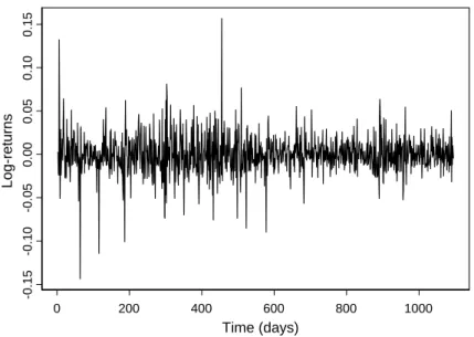
In this period of time the log-returns,rt, are defined by,
rt= ln (Rt+ 1) = ln(Pt)−ln(Pt−1)
0 200 400 600 800 1000
-0.15
-0.10
-0.05
0.00
0.05
0.10
0.15
Log-returns
Time (days)
Figure 4: Time series of log-returns of the Gillette Company stock
Figure 4 represents the log-return behavior of Gillette’s stock prices for the same period. Although the loss of value faced by the company is a feature in-ferred by price behavior, changing volatility pattern is a stylized fact deduced from this picture. It is evident there are two striking behaviors for returns volatility, a broader one from 1999 to the beginning of 2002 and a narrower one from 2002 on. This picture describes a situation that shows more volatil-ity during the time Gillette was losing more value, an expected fact because stockholders are more sensitive when their losses are bigger. Shareholders who detain broader slices of the company’s control are expected to remain un-til the complete company’s selling, otherwise their losses can be even bigger. Probably this explains the company’s diminishing stock prices volatility after 2002.
Models for the log-returns series
For modeling log returns of asset prices models of the classes GARCH and EGARCH are mostly used and estimated, once the residuals and the square of residuals satisfy the autocorrelation principle. The selected estimated model for the series of log-returns of share’ prices of Gillette is the EGARCH(2,1), with:
ˆ
µt=−0.0007
lnhˆt
=−0.1014 + 0.9910 lnhˆt−1
+ 0.338|zt−1| −0.1467zt−1
−0.2973|zt−2|+ 0.0724zt−2
where ˆµtis the MLE estimate of the mean, ˆhtis the MLE estimate of the vari-ance andzt=√ǫtˆ
ht
is the standardized residual deviation. The p-values of the
tests for all parameters are all smaller than 0.001, except the p-value associ-ated with the parameterγ2, which is given by 0.045. For this model the AIC
and BIC values are−4.9383 and−4.9062, respectively.
General Exponential GARCH Model
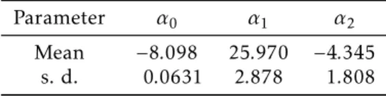
In this section we consider the{rt}t∈Iprocess, wherertis the log-return at time tcentered in zero. In this case we consider two very simple models. The first one is given by the equation
ht= exp (α0+α1|rt−1|+α2rt−2)
has Bayesian parameter estimates (and standard deviations) given in Table 6. For this model, the AIC and BIC values are equal to−3.8590 and−3.8454, respectively.
Table 6: Posterior summaries for General Exponential model
Parameter α0 α1 α2
Mean −8.098 25.970 −4.345 s. d. 0.0631 2.878 1.808
The second one given by the equation
ht= exp
α0+α1|rt−1| 1 2+α2rt
−1+α3rt−2
has Bayesian parameter estimates (and standard deviations) given in Table 7. For this model, theAIC value are equal to−3.8767 andBICvalues are equal to−3.8631. Thus, the last model is better suited by the data using AIC and BIC as the selection criterion, since it has the smallest value.
Table 7: Posterior summaries for General Exponential model
Parameter α0 α1 α2 α3
Mean −8.483 6.937 −6.2050 −6.937 s. d. 0.0972 0.7762 1.9730 0.7762
Stochastic Volatility Model
Assuming the stochastic volatility model introduced in section 4 by equations 4, 5 and 5, withσǫ= 1, and prior distributions 13, 14, 15 and 16 with hyper-parameter values a1=b1=c1=c2= 1 ande2= 100, we have in Table 8, the
posterior summaries of interest based on a final Gibbs sample of size 1000 and a burn-in-sample of 5000 samples using the software WinBugs.
Table 8: Posterior summaries (SV model)
Parameters µ φ ση
Mean −8.076 0.7661 3.132 s. d. 0.09724 0.05706 0.7626
For this model, the AIC and BIC values are−5.3819 and−5.3682, respec-tively. Observe that based on the AIC and BIC values, the SV models with AR(1) structure give a better fit for the log-returns of Gillette, since they have smaller AIC and BIC values than using the general exponential GARCH mod-els. In the same way, based on these criteria, we observe that SV provides a better fit for the log-return time series when compared to the EGARCH(2,1) model.
7
Concluding Remarks
Different volatility models have been introduced in the literature to analyze
financial time series. Using Bayesian methods is a suitable alternative to ana-lyzing the volatility of financial time series, since the complexity of the likeli-hood function can be a problem for obtaining maximum likelilikeli-hood estimates for the parameters of the proposed models, especially when we assume gen-eral exponential GARCH models and SV models.
For the example of financial time series included in this paper, we observe that SV models give better fit for the data, especially for the log-return series. Further studies should be carried on for other applications mainly in the special cases of multivariate time series.
It is important to point out that General Exponential GARCH models or SV models usually provide improvements in the fit of time series data when compared to the usual ARCH or GARCH models as we can see by the results achieved in this paper.
A set of four different models are estimated in this paper for the stock
are confirmed: volatility is an issue to be concerned with and its incidence over the stock prices is skewed. Excess volatility is inferred by its parameters significance and distortion is demonstrated by the signal changes in EGARCH estimates.
Concerning log-returns estimates, Bayesian estimates are a better fit. Among three estimated models, a Bayesian stochastic volatility model representation turns out to be the best one, a conclusion that is based on AIC and BIC crite-ria. Bayesian stochastic volatility model estimates outperform others because introducing prior distributions to each parameter is a more flexible inference procedure. Moreover, the possibility of introducing an order one autoregres-sive structure to represent the noise better fits Gillette’s stock returns.
The obtained results allow us to conclude that an order one autoregressive process is significant in determining returns of this Company in this period of time; its return is almost zero on average and total volatility is expressive, a statement that is confirmed by the estimate ofση. Clearly these results resem-bles the main features of the log-returns contained in Figure 4 and validates the hypotheses of significance of null expected average returns; autoregres-sive behavior for volatility of financial time series and the excess volatility are presented in these time series.
All the estimates provided by ARCH, GARCH and EGARCH class models confirm the expected excess volatilityshowed by financial time series. More-over, the long lasting memory volatility hypothesis is accepted in both cases; i.e. for the error term and for the entire volatility structure. In particu-lar, EGARCH models reflect the leverage effect that weighs more bad news
than good news’ likelihood. Changing estimates signals and their magnitudes strengthen these results.
The magnitudes ofβ1estimates in all models reinforce the idea of time
se-ries integration, a common feature in financial asset prices. However, express-ing the model in returns the problem is overcomed, as expected. Possibly, this finding is a matter for demanding the introduction of a autoregressive struc-ture into the latent variable, what is successfully done when estimating SV Bayesian Models.
Concerning SV Bayesian models, it is clear its results strictly reproduce the main features presented by finamcial asset prices time series. Volatility is an issue, since it is expressive and significant by the estimates presented in table 6. With a coefficient magnitude of 3.132 forσnthe investor can expect a
deviation of approximately 4.78% from the mean return, which is significant for a US stock market perspective.
Autoregressive coefficient is also significant and its estimated value
re-flects the existence of a memory structure on determining returns volatility. Roughly, 75% of a volatility generated in a period of time is transmitted to the following period, which is a despicable mark. Finally, the estimated mean returns resembles the one exhibited in figure 6; i.e. though the estimated coef-ficient is negative and equal to -8.076, we remember this is a result for returns in logarithm, so the real percentage return is close to zero.
Bibliography
Bollerslev, T. (1986), ‘Generalized autoregressive conditional heteroskedas-ticity’,Journal of Econometrics31, 307–327.
Carlin, B. & Louis, T. (2000),Bayes and Empirical Bayes methods for date anal-ysis, Chapman and Hall/ CRC Press, -.
Cepeda, E. & Gamerman, D. (2001), ‘Bayesian modelling of variance het-erogeneity in normal regression models’,Brazilian Journal of Probability and
Statistics14, 207–221.
Engle, R. (1982), ‘Autoregressive conditional heteroscedasticity with esti-mates of the variance of uk inflation’,Econ.50, 987–1007.
Engle, R. (1983), ‘Estimates of the variance of us inflation based upon the arch model’,Journal of Money, Credit, and Banking15(286-301).
Engle, R. F. & Ng, V. (1993), ‘Measuring and testing the impact of news on robert engle volatility’,Journal of Finance48(5), 1749–1778.
Gelfand, A. E. & Smith, A. F. M. (1990), ‘Sampling-based approaches to cal-culating marginal densities’, Journal of the American Statistical Association
85(410), 398–409.
Ghysels, E., Harvey, A. C. & Renault, E. (1996), ‘Stochastic volatility’,
Statis-tical methods in finance. Handbook of Statistpp. 119–191.
Glosten, L., Jannanthan, R. & Runkle, D. (1993), ‘Relationship between the expected value and the volatility of the nominal excess of return on stocks’,
Journal of Finance48, 1779–1802.
Heynen, R., A., K. & T., V. (1994), ‘Analysis of the term structure of implied volatilities’,Journal of Financial and Quantitative Analysis29, 31–56.
Hull, J. & White, A. (1987), ‘The pricing of options on assets with stochastic volatility’,The Journal of Finance42(2), 281–300.
Kim, S., Shephard, N. & Chib, S. (1998), ‘Stochastic volatility: likelihood inference and comparison with arch models’,The Review of Economic Studies
65(3), 361–393.
Lumsdaine, R. (1995), ‘Finite-sample properties of the maximum-likelihood estimator in garch(1,1) and igarch(1,1) models a monte carlo investigation’,
Journal of Business and Economic Statistics13, 1–10.
Meyer, R. & Yu, J. (2000), ‘Bugs for a bayesian analysis of stochastic volatility models’,The Econometrics Journal3(2), 198–215.
Nelson, B. D. (1991), ‘Conditional heterocedasticity in asset returns: A new approach’,Econometrica59(2), 347–370.
Schwarz, G. (1978), ‘Estimation of the dimension of a model’,Annals of Statis-tics6, 461–466.
Shephard, N. (1996), ‘Statistical aspects of arch and stochastic volatility’,
Smith, A. F. M. & Roberts, G. O. (1993), ‘Bayesian computation via the gibbs sampler and related markov chain monte carlo methods (with discussion)’,
Journal of the Royal Statistical Society. B55, 3–23.
Spiegelhalter, D. J., Thomas, A., Best, N. G. & Lund, D. (1999), WinBUGS
User Manual, Cambridge, United Kingdon: MRC Biostatistics Unit.
Taylor, S. (1994), ‘Modelling stochastic volatility: a review and comparative study’,Mathematical finance4, 183–204.