João Paulo Dias
[email protected] Federal University of Santa Catarina Department of Mechanical Engineering 88040-900 Florianópolis, SC, BrazilJosé Luiz Gasche
[email protected] São Paulo State University – College of Ilha Solteira Department of Mechanical Engineering 15385-000 Ilha Solteira, SP, BrazilAndré Luiz Seixlack
[email protected] São Paulo State University – College of Ilha Solteira Department of Mechanical Engineering 15385-000 Ilha Solteira, SP, BrazilMathematical Modeling of the Ester
Oil-Refrigerant R134a Mixture
Two-Phase Flow with Foam Formation
Through a Small Diameter Tube
This work presents a mathematical modeling to study the ester oil ISO VG-10-refrigerant R134a mixture two-phase flow with foam formation through a 3.22 mm ID tube. Based on experimental visualization results, the flow is divided into three regions: a single phase flow at the inlet of the tube; an intermediary bubbly flow region; and a foam flow region at the end of the tube. Numerical results for mass flow rate, pressure and temperature distributions along the flow were compared with experimental data available in literature, showing good agreement. The major discrepancy between the mass flow rate data was about 21%. These results show that the mathematical modeling worked well for predicting the overall characteristics of the flow and can be generically used to other oil-refrigerant mixtures.
Keywords: oil, refrigerant, mixture, compressor, foam
Introduction1
The vapor compression refrigeration system is the most widely used method of producing cooling effects for both air conditioning and food refrigeration industries. This type of system is composed basically of four mechanical components: compressor, evaporator, condenser, and expansion device. Two important fluids complete the system: the refrigerant, which is responsible for the heat exchanges that occur in the condenser and evaporator, and the lubricant oil, whose main purpose is to reduce the friction among the compressor sliding parts.
These two fluids are in constant physical interaction inside the components of the system, producing the formation of a mixture consisting of lubricant oil and refrigerant. The formation of this mixture brings advantages and disadvantages. It is well known that a good miscibility between refrigerant and lubricant oil is required to allow easy return of circulating oil to the compressor, which benefits evaporators, condensers, and expansion devices. In addition, high refrigerant absorption rates in the oil are desirable to diminish the equalizing pressure, which reduces torque and power required for compressor start-up (Prata and Barbosa, 2007). On the other hand, this miscibility can modify the lubrication of sliding parts, the performance of journal bearings, and the leakage of refrigerant gas through the compressor clearances. For example, reduction in load capacity of compressor journal bearings has been observed when oil-refrigerant mixture flow model is used rather than pure oil flow model (Grando, Priest and Prata, 2005).
Two types of mixture can be found in the system. In the evaporator, condenser, and expansion device, where a large amount of refrigerant circulates, a refrigerant-rich mixture is found. The concentration of oil in this type of mixture is small, usually less than 10%. However, the oil can affect the heat exchangers performance taking into account that, at high vapor quality, the amount of oil in the liquid phase can achieve values much higher than 10%. Otherwise, inside the compressor, where lubricant oil is the predominant fluid, an oil-rich mixture prevails. In this case, the oil concentration ratio is commonly larger than 70%.
A literature review on oil-refrigerant mixture studies shows that more emphasis has been given to refrigerant-rich mixtures: Schlager, Pate and Bergles (1987), Eckels and Pate (1991), Hambraues (1995), Cho and Tae (2000), Cho and Tae (2001), Bassi
Paper received 28 July 2009. Paper accepted 10 June 2010. Technical Editor: José Parise
and Bansal (2003), Chen, Won and Wang (2005), and Bandarra Filho, Cheng and Thome (2009). The purpose of these works has been mainly to analyze the oil influence in pressure drop and heat transfer coefficient in condensers and evaporators.
Nomenclature
a = constant of Equation 9, dimensionless b = constant of Equation 9, dimensionless c = constant of Equation 9, dimensionless d = constant of Equation 9, dimensionless f = Darcy friction factor, dimensionless G = mass flux, kg m-2 s-1
m& = mass flow rate, kg s-1
n = foam behavior index, dimensionless p = pressure, Pa
R = tube internal radius, m r = radial coordinate, m T = temperature, oC
u = longitudinal flow velocity, m s-1 us = foam slip velocity at the tube wall, m s-1
u0 = foam velocity in the plug flow region, m s-1
x = mass quality, dimensionless z = tube longitudinal coordinate, m w = refrigerant mass fraction, kgrefrig kgmixt-1
wsat = solubility of refrigerant in oil, kgrefrig kgmixt-1
Greek Symbols
α = void fraction, dimensionless δs = liquid layer thickness, m
ε = tube internal roughness, m φ = metastability factor, dimensionless κ = foam solidity index, Pa sn
µ = absolute viscosity, Pa s ρ = density, kg m-3 σ = standard deviation τe = foam yield stress, Pa
τrz = shear stress, Pa
Subscripts
J. of the Braz. Soc. of Mech. Sci. & Eng. Copyright 2011 by ABCM July-September 2011, Vol. XXXIII, No. 3 / 315 inc = inception
lim = limit s = slip sat = saturated
v = relative to vapor phase
Superscripts
- = relative to homogeneous property * = relative to estimated value
For oil-rich mixtures, however, few works have been reported. Some researchers have focused on the lubricating characteristics of the mixture: Jonsson (1999), Chul Na, Chun and Han (1997), Grando, Priest and Prata (2006). Other researchers have studied the transient processes of absorption and separation (outgassing) of refrigerant in oil, which is useful, for example, to estimate the concentration of refrigerant in the oil stored inside the compressor in the start-up condition: Silva (2004) and Fukuta et al. (2005).
There have been very few studies on oil-rich mixture flow with phase change, which may also be an important issue when the compressor is the focus of the study. A general understanding of the oil-rich mixture flashing flow through small channels is important in order to develop a knowledge basis onto which lubrication and gas leakage models can be built.
One of the primary steps towards constructing a study methodology for the lubrication of compressor parts and gas leakage in the presence of refrigerant outgassing is the investigation of refrigerant-lubricant oil flows in a simple geometry as a straight horizontal tube. The resulting two-phase, two-component flow encompasses very peculiar characteristics and requires special attention as far as its modeling is concerned.
Many efforts have been done in this direction over the last 15 years by Prata and coworkers, and Gasche and coworkers. Experimental works directed to flashing flow of oil-rich mixture through tubes of around 3 mm internal diameter have been performed by Lacerda, Prata and Fagotti (2000), Poiate Jr. and Gasche (2006), Barbosa Jr., Lacerda and Prata (2004), and Castro, Gasche and Prata (2009). The two-phase characteristic of the flow is the most important aspect found in all those works. In addition, foam flow pattern is always observed as the void fraction reaches high values, usually larger than 0.7. Together with the pressure drop, a significant temperature drop due to the outgassing is also noticed.
Modeling works involving the flashing flow of oil-rich mixture also have been reported. The first model has been developed by Gasche (1996) to estimate the R22 refrigerant leakage through the radial clearance (convergent-divergent channel) in rolling piston compressors. Based on visualization results, the mixture flow was divided in two regions: a conventional two-phase flow at the inlet of the channel, for void fraction lower than 0.7, and a foam flow region for void fractions larger than 0.7. In the conventional two-phase flow region, the classical homogeneous model was applied to predict the pressure profile along the flow for a prescribed mass flow rate. The foam flow model proposed by Calvert (1990) was used for modeling the foam flow region. Due to the lack of information for oil-refrigerant mixture foams, aqueous foam parameters were used to apply the model. In both regions the flow was considered to be isothermal.
Based on the experimental results obtained by Lacerda, Prata and Fagotti (2000), who observed large temperature reduction along the flow, and on the two-phase mixture flow model proposed by Gasche (1996), Grando and Prata (2003) have developed a model including the energy equation in order to determine also the temperature distribution along the flow. The authors have developed a mathematical model to predict the flow of a mixture composed by mineral oil and refrigerant R12 flowing through a 6 m long, 3 mm
internal diameter tube. The flow was divided in three regions: a sub-saturated liquid mixture (a mixture having a refrigerant mass fraction lower than the saturated mixture) flow at the inlet of the tube, an intermediary conventional two-phase flow region for void fractions lower than a prescribed value, and a foam flow region for void fractions larger than the prescribed value at the end of the tube. In the liquid mixture flow, the momentum equation was simplified for the case of completely developed flow considering the balance only between the pressure and friction forces. In both conventional two-phase flow and foam flow regions, the same model proposed by Gasche (1996) for the momentum equation was used. The aqueous foam parameters were also used by the authors to analyze the flow characteristics. The model has been validated by using the experimental data obtained by Lacerda, Prata and Fagotti (2000).
The major contribution of the work performed by Grando and Prata (2003) was the inclusion of the energy equation for modeling the two-phase flow of oil-refrigerant mixtures. The limitation of the model is that the authors have used aqueous foam parameters in order to study the flow. It would be useful to verify, even if aqueous foam parameters were still used, if the model can be generalized to other oil-refrigerant mixtures, mainly for mixtures of current engineering application.
The purpose of this work is to verify if the mathematical model developed by Grando and Prata (2003) can be applied for a mixture composed by an ester oil and refrigerant R134a (a mixture widely used in vapor refrigeration systems) flowing through a small diameter tube. The model was experimentally validated by using the data obtained by Castro, Gasche and Prata (2009), showing good agreement between numerical and experimental results.
Mathematical Modeling
The proposed model was based on the flow visualization results obtained by Lacerda, Prata and Fagotti (2000), Poiate Jr. and Gasche (2006), and Castro and Gasche (2006), for the mixture flow through a straight long tube with constant internal diameter. These results have indicated the existence of three flow patterns along the tube: a liquid single-phase region at the inlet region of the tube, an intermediary region of bubbly flow pattern, and a foam flow region at the exit of the tube. Figure 1 depicts schematically these flow patterns, based on the work of Castro and Gasche (2006).
Single-phase flow
Bubbly flow
Foam flow
Figure 1. Flow patterns for the oil-refrigerant mixture flow through a straight long tube.
The mathematical model was developed adopting the following assumptions: (i) one-dimensional, fully developed and steady state flow; (ii) impermeable and adiabatic tube walls; (iii) the liquid phase is formed by oil and liquid refrigerant, while the vapor phase is considered to be formed only by refrigerant gas; (iv) the liquid mixture is treated as an ideal solution. Using the cylindrical coordinate system (r,z), the governing equations of the problem, which are the mass conservation, momentum, and energy conservation equations, can be written as the following (Dias, 2006):
2d du 0
u u
(
)
2 1
rz
dp d d
u r
dz dz r dr
ρ τ
= + (2)
(
)
1 l
v l
T l
p h
dp d dp
x h h
dz dz p dz
dT
h dz
T
ρ − − −∂∂
=
∂ ∂
(3)
Equations (1)-(3) were written in different forms when modeling each flow region depicted in Fig. 1.
Single-phase flow region
In the single-phase region, the pressure drop is caused exclusively by the fluid viscous stresses. Thus, one can simplify Eq. (2) to:
(
)
1 rz
dp d
r
dz =r dr τ (4)
The viscous term can be represented by using the Darcy friction factor:
(
)
21
2 rz
l
dp d f G
r
dz=r dr τ = − ρD (5)
The friction factor, f, was calculated using the correlation proposed by Churchill (1977), which is valid for both laminar and turbulent regimes:
(
)
1/12 12
3 / 2
1 1
8 1
8 Re f
A B
= +
+
(6a)
(
)
16
1 0,9
1 2.457 ln
7
0.27 / Re
A
D ε
=
+
(6b)
16 1
37530 Re B =
(6c)
where the Reynolds number is defined as:
4 Re
l m
D µ π
= ɺ (7)
The density and viscosity of the liquid phase, ρl and µl, used in
Eqs. (5) and (7), respectively, depend on the refrigerant mass fraction, w, which is defined as the mass of the liquid refrigerant dissolved in oil, mlr, divided by the total mass of the liquid mixture, ml:
lr
l m w
m
= (8)
The refrigerant mass fraction in the single-phase flow region was assumed to be smaller than the saturation concentration, also called solubility, wsat(p,T), which depends on the pressure and
temperature of the mixture and was calculated by Eq. (9). Its value must be known at the inlet of the tube, win, in order to calculate the
density and viscosity of the liquid.
p p
a exp c exp
b d
sat
w = − + −
(9)
( )
-4 18
a=3.74 10 +5,78 10− exp T (9a)
-3 T -2 T
b 9.25 10 exp 9.21 10 exp
7.20 107.31
= − −
(9b)
-3 2
c=8.193−2.65 10 T (9c)
T T
d 0.174 exp 0.828 exp
14.275 38.540
= − −
(9d)
where wsat is given in %, p in bar, and T in ºC. These equations are
applicable to 0 < p < 7 bar and 0 < T < 40ºC.
For the single-phase flow region, it is reasonable to assume that the flow is isothermal, which means that the temperature gradient in Eq. (3) is zero.
Integrating Eq. (4) from an initial value of the pressure at the inlet of the tube, one can calculate the pressure profile in the single-phase flow region. In this case, the procedure adopted was the Euler method.
Bubbly flow region
Figure 2 schematically shows the behavior of both the solubility of the refrigerant in oil, wsat(p,T), and the refrigerant mass fraction,
w, along the flow in the single-phase flow region. The refrigerant solubility depends on the pressure and temperature, diminishing as the pressure decreases and temperature increases. The graph shows that at the inlet of the tube, for z = 0, the mass fraction of the refrigerant in oil, w, is smaller than its solubility for the local pressure and temperature, wsat(p,T). It can be seen that the
refrigerant solubility (solid line) diminishes along the flow as the pressure decreases due the friction forces, while the refrigerant mass fraction remains constant along the flow (dashed line) until it reaches the point TPinc where w = wsat(p,T). After this position, any
further reduction in the refrigerant solubility, which is the maximum amount of refrigerant that the mixture can keep dissolved, produces the formation of bubbles, giving rise to two-phase flow.
J. of the Braz. Soc. of Mech. Sci. & Eng. Copyright 2011 by ABCM July-September 2011, Vol. XXXIII, No. 3 / 317 The homogeneous model was used to predict the characteristics
of the two-phase flow region. In this model, the two-phase flow is substituted by a single-phase flow that contains average physical properties, ρ and µ, which are determined by using the physical properties of the gas phase, ρv and µv, and the liquid phase, ρl and µl. Therefore, Eq. (2) for momentum balance can still be used. However, there will be the influence of two terms in the total pressure gradient: the frictional force and the accelerational force, which is caused by the density change along the flow as the amount of gas formed increases. Equation (2) for momentum balance was written differently by using both the mass conservation equation and the Darcy friction factor, resulting in the following equation:
2 2
2
dp G d f G
dz dz D
ρ
ρ ρ
= −
(10)
The friction factor, f, was calculated by Eq. (6) and the Reynolds number was determined by:
4
Re m
D µπ
= ɺ (11)
The average density, ρ, was calculated from the properties of vapor and liquid phases as follows:
(
1)
v l
ρ αρ= + −α ρ (12)
where α is the void fraction of the flow, which is defined as the ratio of the gas flow cross-sectional area to the total cross-sectional area. Considering the liquid and vapor phases flowing at the same velocity, which is the basic assumption of the homogeneous model, the local void fraction results in:
1 1
1 1 v
l x α
ρ ρ =
+ −
(13)
Assuming that the liquid mixture remains consistently saturated with refrigerant, the local quality of the flow, x, can be calculated by using the mass conservation of oil and refrigerant between two consecutive points: TPinc, where the mass fraction is still equal to the
mass fraction at the inlet of the tube, win, and any downstream
position, where the mass fraction is equal to the local solubility, wsat(p,T). This mass balance results in the following equation for the
local quality:
( , )
1 ( , )
in sat
sat
w w p T
x
w p T
− =
− (14)
There are many correlations to estimate the average viscosity, µ, in Eq. (11): Davidson et al. (1943) apud Chang and Ro (1996), Akers et al. (1959) apud Yan and Lin (1998), Isbin et al. (1958), Cichitti et al. (1960), Dukler et al. (1964), Beattie and Whalley (1981) apud Walley (1987), and Lin et al. (1991) apud Wongwises and Pirompack (2001). Considering the experimental-numerical RMS difference for mass flow rate and pressure and temperature distributions as criterion, the correlation proposed by Dukler et al. (1964), given by Eq. (15), produced the best results for the present model.
(
)
(
)
/ 1 /
/ 1 /
v v l l
v l
x x
x x
µ ρ µ ρ
µ
ρ ρ
+ − =
+ − (15)
Equations (3) and (10) were solved simultaneously to provide the temperature and pressure distributions along the bubbly flow region.
Foam flow region
From the point TPinc, the void fraction of the bubbly flow starts
to continuously increase in the z direction. As the void fraction reaches a limiting value, αlim, the flow pattern changes from bubbly
to foam flow. The viscous stress, τrz, is the only difference between
the bubbly flow modeling and the foam flow modeling. Due to the lack of information about the viscous stress for oil-refrigerant mixture foam flow, the correlation proposed by Calvert (1990) for aqueous foam was used in this work.
n
rz e
du dr
τ =τ +κ
(16)
where τe is the foam yield stress, κ is the consistency parameter, and
n is the behavior index of the foam.
Isolating the viscous term of Eq. (2) and integrating it along the radial coordinate one can obtain the following equation for the shear stress:
(
)
2
0 0
1 1
/
r r
rz
dp d
u rdr g dp dz rdr
r dz dz r
ρ
τ = − = −
∫
∫
(17)As can be observed in Eq. (17), the function g is the frictional pressure drop, written as a function of the total pressure drop, dp/dz. In the center line of the flow, for r = 0, the shear stress is zero by definition, and Eq. (17) reduces to:
(
/)
2 rzr g dp dz
τ = − (18)
In the above equation, g(dp/dz) always exhibits positive values. Therefore, using the absolute value in Eqs. (16) and (18), one can write:
(
)
1 1
/ 2
n
n e
du r
g dp dz
dr κ τ
−
= −
(19)
According to the foam flow profile described by Calvert (1990) and depicted in Fig. 3, foam flow presents two regions: a deformation region near the tube wall, where the flow shear stress, τrz, is larger than the foam yield stress, τe, and a plug flow region, in
which the flow shear stress is smaller than the foam yield stress. Integrating Eq. (19) in both these regions separately, the foam radial velocity profile results in:
For the foam deformation region:
( )
1 1 1
2
1 2 2
n n
n n n
s e e
n R r
u r u g g
g n
κ− τ + τ +
= + − − −
+
For the plug flow region:
1 1
0
2
1 2
n
n n
s e
n R
u u g
g n
κ− τ +
= + + −
(21)
Figure 3. Representation of the Calvert (1990) foam modeling.
In the same model proposed by Calvert (1990), there is a small layer of liquid near the wall. The author has proposed to substitute this liquid layer by a slip velocity, us, to establish the foam velocity
profile. Furthermore, the author has considered that the velocity profile in this layer is linear, which results in the following relation for the slip velocity:
2 s s
l R
u g δ
µ
= (22)
In order to obtain the total pressure gradient, the total mass flow rate can be calculated using the foam velocity profiles, Eqs. (20) and (21). Thus, the mass flow rate results in:
( )
0
0
0 0
2 2
R R
R
mɺ =
∫
ρu πrdr+∫
ρu r πrdr (23)which can be organized as:
1 2 3 4
mɺ =mɺ +mɺ +mɺ +mɺ (24)
where the subscripts 1, 2, 3, and 4 are used just to represent the four terms appearing after the integration of Eq. (23). In Eq. (24), each term on the right side is an implicit function of the pressure gradient through the function g:
(
)
31 1 /
2 s
l R
m F dp dz ρπ δ g
µ
= =
ɺ (25)
(
)
1 1
2
2 2
2 /
1 2
n
n n
e
R n R
m F dp dz g
g n
ρπ κ− τ +
= = + −
ɺ (26)
(
)
1 2 1
2
3 3 3
16 /
2
1 2 1
n
n n
e
e
n R
m F dp dz g
g n n
ρπ κ τ− τ +
= = − −
+ +
ɺ (27)
(
)
1 3 1
2
4 4 3
16 /
2
1 2 1
n
n n
e
n R
m F dp dz g
g n n
ρπ κ− τ +
= = − −
+ +
ɺ (28)
A direct solution for the total pressure drop for a given mass flow rate is not possible by using Eq. (24). Therefore, an iterative numerical method needs to be applied to obtain the desired solution. Based on an estimate value for the total pressure gradient, (dp/dz)*, an updated value can be calculated by using the Newton-Raphson method through Eq. (29).
(
)
(
)
* *
*
/
' / F dp dz dp dp
dz= dz −F dp dz (29)
where F dp dz'
(
/ *)
is the derivate of Eqs. (25)-(28). In this work, the pressure gradient of Eq. (29) was solved until a convergence value of 10-7 was found. The simultaneous solution of Eqs. (29) and (3) provides the pressure and temperature distributions along the foam flow region.Numerical Solution Methodology
Figure 4 shows the numerical solution algorithm used for solving the problem. The numerical procedure starts with the definition of the tube’s geometrical parameters, foam parameters, and inlet flow data as pressure gradient, pressure, and temperature.
J. of the Braz. Soc. of Mech. Sci. & Eng. Copyright 2011 by ABCM July-September 2011, Vol. XXXIII, No. 3 / 319 The flow properties as refrigerant mass fraction, density,
viscosity and enthalpy were calculated by the correlations for the liquid mixture proposed by Castro, Gasche and Prata (2009). All refrigerant properties were calculated using the package REFPROP (MacLinden et al., 1998).
The problem was solved step-by-step along the flow domain, which was divided into 286 elements. The pressure and temperature at position z+∆z, pi+1 and Ti+1 were calculated by knowing the
pressure and temperature in certain position z, pi and Ti, and the
appropriate equations for the pressure and temperature gradients, (dp/dz)i and (dT/dz)i, using the Euler method, Eqs. (30) and (31), are
1
i i
i dp
p p z
dz ∆
+ = + (30)
1
i i
i dT
T T z
dz ∆
+ = + (31)
Therefore, using the proposed algorithm, the pressure and temperature profile along the flow can be obtained.
Results and Discussion
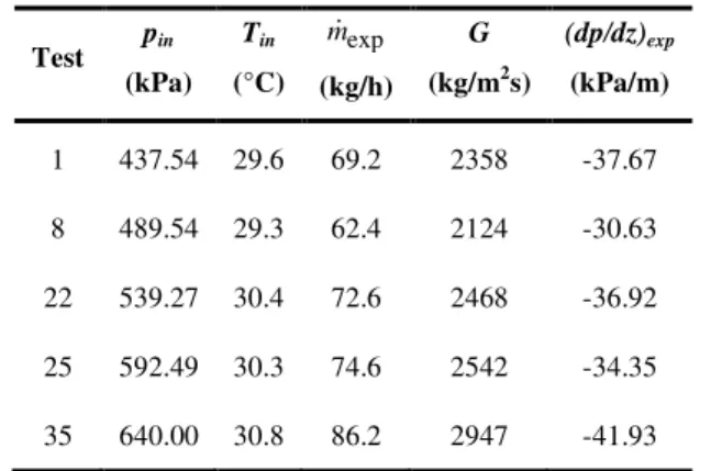
Firstly, the validation of the mathematical model was carried out. In this work, the validation process was accomplished by comparing the numerical results with the experimental data given by Castro, Gasche and Prata (2009) for a mixture composed of ester oil ISO VG10 and refrigerant R134a flowing through a 3.22 mm (±0.03 mm) internal diameter tube. Table 1 presents the operational conditions of the tests performed by the authors, which were used here to validate the mathematical model. The experimental uncertainties for pressure and temperature measurement are ±2 kPa and ±0.5°C, respectively (Castro, Gasche and Prata, 2009). The experimental uncertainties for mass flow rates and mass flux are 5% of the measured values, and the experimental uncertainty for pressure gradients at the tube inlet is ±2 kPa.
Table 1. Experimental tests used for validating the mathematical model.
Test pin (kPa)
Tin
(°C)
exp
mɺ
(kg/h) G
(kg/m2s)
(dp/dz)exp
(kPa/m)
1 437.54 29.6 69.2 2358 -37.67
8 489.54 29.3 62.4 2124 -30.63
22 539.27 30.4 72.6 2468 -36.92
25 592.49 30.3 74.6 2542 -34.35
35 640.00 30.8 86.2 2947 -41.93
Figures 5 to 14 present comparisons of numerical and experimental results for pressure and temperature distributions of these tests. The error bars in those figures accounts for the variation of pressure and temperature during the tests, based on the 2σ criteria, and also for the uncertainty of the respective measurements, that is, the uncertainty of the pressure transducer (Im = ±2 kPa) and temperature transducer (Im = ±0.5°C). The final result was grouped as ±[(2σ)2+(Im)2]1/2. In order to obtain the numerical results, the foam parameters suggested by Grando and Prata (2003) were used: τe = 1 Pa, κ = 1.168 Pa sn, n = 0.4, δs = 5.0
µm, and αlim = 0.6. The foam parameters suggested by Grando and
Prata (2003) were the best values encountered by the authors considering the comparison between the simulation results and the experimental data obtained by Lacerda, Prata and Fagotti (2000) for the mineral oil/R12 mixture flow.
0 1 2 3 4 5 6
150 200 250 300 350 400 450
Experimental Dukler
p
in=437.54 kPa
Tin=29.6 °C win=0.6154wsat
G=1956 kg/m2s
p
(k
P
a
)
z(m)
Figure 5. Pressure distribution comparison for test 1.
0 1 2 3 4 5 6
23 24 25 26 27 28 29 30
pin=437.54 kPa
T
in=29.6 °C
win=0.6154wsat
G=1956 kg/m2s
Experimental Dukler
T
(°
C
)
z(m)
Figure 6. Temperature distribution comparison for test 1.
0 1 2 3 4 5 6
150 200 250 300 350 400 450 500
p
(k
P
a
)
z(m)
pin=489.54 kPa
Tin=29.3 °C win=0.716wsat
G=2141 kg/m2s
Experimental Dukler
Figure 7. Pressure distribution comparison for test 8.
of the experimental data used in this work to validate the model for the ISO VG10/R134a mixture flow. As the aqueous foam parameters were used as basic values for both models because of the lack of information for oil/refrigerant mixture foams, this is a research area of great interest for future works.
0 1 2 3 4 5 6
22 23 24 25 26 27 28 29 30
pin=489.54 kPa
Tin=29.3 °C win=0.716wsat
G=2141 kg/m2s
Experimental Dukler
T
(°
C
)
z(m)
Figure 8. Temperature distribution comparison for test 8.
0 1 2 3 4 5 6
200 250 300 350 400 450 500 550
Experimental Dukler
pin=539.27 kPa
Tin=30.44°C win=0,647wsat
G=2516 kg/m2s
p
(k
P
a
)
z(m)
Figure 9. Pressure distribution comparison for test 22.
0 1 2 3 4 5 6
22 23 24 25 26 27 28 29 30 31
Experimental Dukler
pin=539.27 kPa
Tin=30.44°C win=0,647wsat
G=2516 kg/m2s
T
(°
C
)
z(m)
Figure 10. Temperature distribution comparison for test 22.
Two points are highlighted in these comparisons. The first point is related to the experimental data obtained by Castro, Gasche and Prata (2009). In this experimental work, a saturated mixture – a mixture with w = wsat(pin,Tin) – is stored in a high pressure tank and
flows through a 3.22 internal diameter, 6 m long tube. In order to avoid outgassing (bubble formation) before the liquid mixture reached the tube, a mass flow meter was not used by Castro, Gasche and Prata (2009) to measure the mass flow rate. Instead, the mass flow rate was calculated by using the linear pressure gradient measured at the inlet region of the flow, where the mixture was still in the liquid state and the flow was completely developed. The average velocity used to determine the mass flow rate was calculated using Eq. (32):
1/ 2
exp
2
l
D dp
V
f dz ρ
= −
(32)
where D is the tube diameter, ρl is the liquid mixture density
calculated at the inlet temperature, pressure, and refrigerant solubility, f is the friction factor calculated by the equation proposed by Churchill (1977), and dp/dz is the pressure gradient along the flow direction measured at the linear portion of the pressure distribution. The Reynolds number used to calculate the friction factor was defined as:
Re l
l VD ρ
µ
= (33)
where µl is the absolute viscosity of the liquid mixture at the inlet
temperature, pressure, and refrigerant solubility.
0 1 2 3 4 5 6
150 200 250 300 350 400 450 500 550 600
pin=592.49 kPa
Tin=30.3°C win=0.68wsat
G=2608 kg/m2s
Experimental Dukler
p
(k
P
a
)
z(m)
Figure 11. Pressure distribution comparison for test 25.
0 1 2 3 4 5 6
18 20 22 24 26 28 30 32
z(m) Experimental Dukler
pin=592.49 kPa
Tin=30.3°C win=0.68wsat
G=2608 kg/m2s
T
(°
C
)
J. of the Braz. Soc. of Mech. Sci. & Eng. Copyright 2011 by ABCM July-September 2011, Vol. XXXIII, No. 3 / 321
0 1 2 3 4 5 6
200 250 300 350 400 450 500 550 600 650
pin=640.00 kPa
Tin=30.8°C win=0.63wsat
G=2710 kg/m2s
Experimental Dukler
p
(k
P
a
)
z(m)
Figure 13. Pressure distribution comparison for test 35.
0 1 2 3 4 5 6
20 22 24 26 28 30 32
Experimental Dukler
pin=640.00 kPa
T
in=30.8°C
win=0.63wsat
G=2710 kg/m2s
T
(°
C
)
z(m)
Figure 14. Temperature distribution comparison for test 35.
As can be seen in Eqs. (32) and (33), the experimental mass flow rate was calculated by using the physical properties of a saturated mixture, ρl and µl, which are dependent on the inlet
solubility, wsat(pin,Tin). However, the numerical results were
obtained for the same inlet experimental pressure gradient, but for a lower inlet refrigerant mass fraction, w < wsat(pin,Tin). As the mass
flow rate is dependent on the refrigerant mass fraction, the numerical mass flow rate is different from the experimental one. Nevertheless, the inlet pressure gradient is the same for both experimental and numerical results. The reason for using a lower refrigerant mass fraction at the inlet of the flow to obtain the numerical results is the second point to be pointed out.
For a saturated mixture in the tank, it would be expected that the bubble formation started exactly at the inlet of the tube, after the very first pressure drop occurred. However, the visualization results have shown the existence of a 3 m long single-phase flow in the inlet region of the tube. This type of result characterizes the metastability phenomenon.
For a pure substance, metastable states can exist in non-equilibrium condition when vapor is sub-cooled below its equilibrium saturation temperature or liquid is superheated above its equilibrium saturation temperature for a given pressure.
In the case of the mixture, it is assumed that the saturated mixture is in thermodynamic equilibrium at the inlet of the tube. Therefore, if the mixture remained in thermodynamic equilibrium continuously, any pressure drop would cause bubble inception due to the solubility reduction of the refrigerant in oil, and the bubbly flow would start as soon as the flow entered the tube. As
single-phase flow does exist in the experimental tests, it must be predicted by the mathematical model.
One way to model the metastability phenomenon that occurs in the single-phase flow region is to assume that the refrigerant mass fraction at the inlet of the tube is smaller than its solubility, win =
φ.wsat(pin,Tin), with φlower than 1, as shown in Fig. 2. After the
bubble inception point, TPinc, both the liquid mixture and refrigerant
gas were considered to be in thermodynamic equilibrium.
Therefore, the procedure for obtaining the numerical results has to take into account both of these effects. The following algorithm was chosen to solve the problem:
1. The experimental inlet pressure gradient was fixed, (dp/dz)exp;
2. An initial value for the parameter φ was estimated; 3. The inlet refrigerant mass fraction was calculated, win;
4. The mass flow rate was determined;
5. The total pressure and temperature drops (pressure and temperature drops along the entire tube) were compared with the experimental data;
6. If these results were within a previous specified tolerance then the solution was found;
7. Contrarily, one must return to item 2 and iterate until the desired convergence is reached.
For test 1, φ = 0.6154 was the factor value that produced the best agreement between the experimental and numerical results for the given inlet pressure gradient. In this case, the mass flow rate calculated was 57.3 kg/h. In Table 1, one can notice that the experimental mass flow rate calculated by Castro, Gasche and Prata (2009) was 21% larger (69.2 kg/h). Despite this difference, it is important to point out that the inlet pressure gradient is equal in both cases.
Considering all the results shown in Figs. 5-14, one can conclude that the mathematical model was able to suitably predict the overall flow characteristics. However, for lack of specific information for the ester oil ISO VG10-refrigerant R134a mixture, the foam parameters suggested by Grando and Prata (2003) were employed in all tests. It would be important to analyze the numerical results for the different values of these parameters in order to verify their influence on the predictions.
The foam yield stress, τe, was varied from 1 to 4 Pa, and the
liquid layer thickness, δs, was modified from 1 to 10 µm, resulting
in insignificant changes in the pressure and temperature distributions.
The limit value of the void fraction for foam flow inception varied from 0.5 to 0.8. The results showed that its influence is minimal for the lower inlet pressure and increases for higher inlet pressures, as shown in Figs. 15 and 16. The best value for this parameter is 0.7, when the pressure and temperature profiles are taken into account.
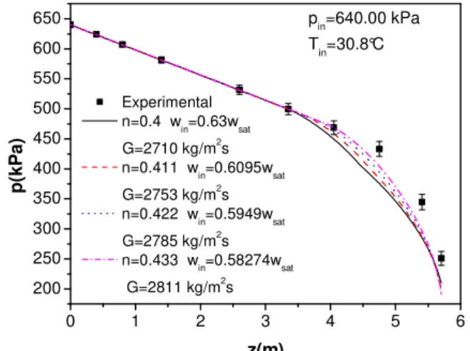
Parameter n varied from 0.4 to 0.433 and presented major influence for test 35, as shown in Figs. 17 and 18. It can be observed that the best agreement was obtained for n = 0.433.
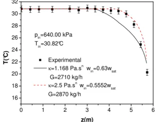
Parameter κ plays the most important role in all of them. Figures 19 and 20 depict pressure and temperature distributions for κ = 1.168 Pa sn and κ = 2.5 Pa sn. It can be noticed that the best agreement was obtained for the larger values.
0 1 2 3 4 5 6 200
250 300 350 400 450 500 550 600 650
pin=640.00 kPa Tin=30.8°C Experimental
αlim=0.5 win=0.64wsat G=2690 kg/m2s
αlim=0.6 win=0,63wsat G=2710 kg/m2s
αlim=0.7 win=0,615wsat G=2741 kg/m2s
αlim=0.8 win=0.589wsat G=2798 kg/m2s
p
(k
P
a
)
Figure 15. Influence of the αααlimα in the pressure distribution for test 35.
0 1 2 3 4 5 6
20 22 24 26 28 30 32
pin=640.00 kPa Tin=30.8°C
Experimental αlim=0.5 w
in=0.64wsat G=2690 kg/m2s
αlim=0.6 w in=0,63wsat G=2710 kg/m2
s αlim=0.7 win=0,615wsat G=2741 kg/m2s
αlim=0.8 win=0.589wsat G=2798 kg/m2s
T
(°
C
)
z(m)
Figure 16. Influence of the αααlimα in the temperature distribution for test 35.
0 1 2 3 4 5 6
200 250 300 350 400 450 500 550 600
650 pin=640.00 kPa
Tin=30.8°C
Experimental n=0.4 win=0.63wsat G=2710 kg/m2s
n=0.411 w
in=0.6095wsat G=2753 kg/m2s
n=0.422 win=0.5949wsat G=2785 kg/m2s
n=0.433 win=0.58274wsat G=2811 kg/m2s
p
(k
P
a
)
z(m)
Figure 17. Influence of the parameter n in the pressure distribution for test 35.
Conclusions
In this work, the mathematical model proposed by Grando and Prata (2003) was used to simulate the ester oil ISO VG10-refrigerant R134a mixture two-phase flow through a straight 3.22 mm internal diameter, 6 m long tube. Based on experimental flow visualization results, three flow patterns were considered to predict the flow: an inlet liquid single-phase region, an intermediary bubbly flow region, and a foam flow region at the end of the tube. In order to simulate the
single-phase flow region at the inlet of the flow, the metastability phenomenon was considered. The homogeneous flow model together with the viscosity correlation given by Dukler et al. (1964) was used to simulate the bubbly flow region. The foam flow model proposed by Calvert (1990), with aqueous foam parameters, was used to calculate the foam flow region.
Results for mass flow rate, pressure and temperature profiles along the flow were numerically obtained through the mathematical model and compared to experimental data from Castro, Gasche and Prata (2009), showing good agreement. The major discrepancy between the mass flow rate data was about 21%.
For lack of specific information about the foam parameters for the ester oil ISO VG10-refrigerant R134a mixture, aqueous foam parameters were employed in all tests. The parametric analysis performed in this work indicates that the parameters n and κ play the major roles in the simulations. Therefore, these parameters should be better known through experimental data in order to enhance the numerical results obtained by the proposed mathematical modeling for both oil-refrigerant mixtures studied in this work.
These results show that the mathematical modeling worked well for predicting the overall characteristics of the ester oil-refrigerant R134a mixture. As the same model has also been validated by Grando and Prata (2003) for another type of mixture, this is a good indication that it can be generalized for predicting the two-phase flow with foam formation for other oil-refrigerant mixtures, mainly if the actual values of the foam parameters are employed.
0 1 2 3 4 5 6
16 18 20 22 24 26 28 30 32
z(m)
pin=640.00 kPa
Tin=30.8°C
Experimental n=0.4 w
in=0.63wsat G=2710 kg/m2s
n=0.411 w
in=0.6095wsat G=2753 kg/m2
s n=0.422 win=0.5949wsat G=2785 kg/m2s
n=0.433 w
in=0.58274wsat G=2811 kg/m2sh
T
(°
C
)
Figure 18. Influence of the parameter n in the temperature distribution for
test 35.
0 1 2 3 4 5 6
200 250 300 350 400 450 500 550 600 650
p
(k
P
a
)
z(m)
pin=640.00 kPa
Tin=30.82°C
Experimental
κ=1.168 Pa.sn win=0.63wsat G=2710 kg/h
κ=2.5 Pa.sn w
in=0.5552wsat
G=2870 kg/h
J. of the Braz. Soc. of Mech. Sci. & Eng. Copyright 2011 by ABCM July-September 2011, Vol. XXXIII, No. 3 / 323
0 1 2 3 4 5 6
16 18 20 22 24 26 28 30 32
pin=640.00 kPa
Tin=30.82°C Experimental
κ=1.168 Pa.sn w
in=0.63wsat
G=2710 kg/h
κ=2.5 Pa.sn win=0.5552wsat G=2870 kg/h
T
(°
C
)
z(m)
Figure 20. Influence of the parameter κκκκin the temperature distribution for test 35.
Acknowledgements
The authors thank CAPES and FAPESP for the financial support of this work.
References
Bandarra Filho, E.P., Cheng, L. and Thome, J.R., 2009. “Flow Boiling Characteristics and Flow Pattern Visualization of Refrigerant/Lubricant Oil Mixture”, International Journal of Refrigeration, Vol. 32, pp. 185-202.
Barbosa Jr., J.R., Lacerda, V.T. and Prata, A.T., 2004, “Prediction of Pressure Drop in Refrigerant-Lubricant Oil Flows with High Contents of Oil and Refrigerant Outgassing in Small Diameter Tube”, International Journal of Refrigeration, No. 27, pp. 129-139.
Bassi, R. and Bansal, P.K., 2003, “In-Tube Condensation of Mixture of R134a and Ester Oil: Empirical Correlations”, International Journal of Refrigeration, Vol. 26, No. 4, pp. 402-409.
Calvert, J.R., 1990, “Pressure Drop for Foam Flow Through Pipes”,
International Journal of Heat and Fluid Flow, Vol. 11, No. 3, pp. 236-241. Castro, H.O.S., 2006, “Experimental Characterization of the Two-phase Flow with Foam Formation of the Oil-refrigerant R134a Mixture Through a Constant Circular Cross Section Tube” (in Portuguese), Ms. Dissertation, Unesp-Faculdade de Engenharia de Ilha Solteira, Ilha Solteira-SP, Brazil.
Castro, H.O.S. and Gasche, J.L., 2006, “Foam Flow of Oil-Refrigerant R134a Mixture in a Small Diameter Tube”, Proceedings of the 13th
International Heat Transfer Conference – IHTC13, Sydney, Australia, paper 359.
Castro, H.O.S., Gasche, J.L. and Prata, A.T., 2009, “Pressure Drop Correlation for Oil-Refrigerant R134a Mixture Flashing Flow in a Small Diameter Tube”, International Journal of Refrigeration, Vol. 32, pp. 421-429.
Chang, S.D. and Ro, S.T., 1996, “Pressure Drop of Pure HFC Refrigerants and their Mixtures Flowing in Capillary Tubes”, International Journal of Multiphase Flow, Vol. 22, No. 3, pp. 551-561.
Chen, I.Y., Won, C.L. and Wang, C.C., 2005, “Influence of Oil on R-410A Two-Phase Frictional Pressure Drop in a Small U Type Wavy”,
International Communications in Heat and Mass Transfer, Vol. 32, No. 6, pp. 797-808.
Cho, K. and Tae, S.J., 2000, “Evaporation Heat Transfer for R-22 and R-407C Refrigerant-Oil Mixture in a Microfin Tube with a U-Bend”,
International Journal of Refrigeration, Vol. 18, No. 2, pp. 219-231.
Cho, K. and Tae, S.J., 2001, “Condensation Heat Transfer for R-22 and R-407C Refrigerant-Oil Mixture in a Microfin Tube with a U-Bend”,
International Journal of Heat and Mass Transfer, Vol. 44, No. 11, pp. 2043-2051.
Chul Na, B., Chun, K.J. and Han, D.C., 1997, “A Tribological Study of Refrigeration Oils Under HFC-134a Environment”, Tribology International, Vol. 30, No. 9, pp. 707-716.
Churchill, S.W., 1977, “Friction-Factor Equation Spans all Fluid-Flow Regimes”, Chemical Engineering, No. 7, pp. 91-92.
Dias, J.P., 2006, “Computational Simulation of the Oil-refrigerant R134a Mixture Two-phase Flow with Foam Formation Through a Constant Circular Cross Section Tube” (in Portuguese), Ms. Dissertation, Unesp-Faculdade de Engenharia de Ilha Solteira, Ilha Solteira-SP, Brazil.
Eckels, S.J. and Pate, M.B., 1991, “In-Tube Evaporation and Condensation of Refrigerant-Lubricant Mixtures of HFC-134a and CFC-12”,
ASHRAE Transactions, Vol. 97, Part 2, pp. 62-70.
Fukuta, M., Yanagisawa, T., Omura M. and Ogi, Y., 2005, “Mixing and Separation Characteristics of Isobutane with Refrigeration Oil”,
International Journal of Refrigeration, Vol. 28, No. 7, pp. 997-1005. Gasche, J.L., 1996, “Oil and Refrigerant Flow through the Radial Clearance of Rolling Piston Compressors” (in Portuguese), Dr. Eng. Thesis, Federal University of Santa Catarina, Florianópolis-SC, Brazil.
Grando, F.P. and Prata, A.T., 2003, “Computational Modeling of Oil-Refrigerant Two-Phase Flow with Foam Formation in Straight Horizontal Pipes”, Proceedings of the 2nd International Conference on Heat Transfer,
Fluid Mechanics and Thermodynamics – HEFAT, Zambia, paper GF2. Grando, P., Priest, M. and Prata, A.T., 2005, “Lubrication in Refrigeration Systems: Performance of Journal Bearings Lubricated with Oil and Refrigerant Mixtures”, Life Cycle Tribology, Proc. 31st Leeds-Lyon
Symposium on Tribology, Leeds 2004, Tribology and Interface Engineering Series, Elsevier, Amsterdam, pp. 481-491.
Grando, F.P., Priest, M., Prata, A.T., 2006, “A Two-Phase Flow Approach to Cavitation Modeling in Journal Bearings”, Tribology Letters, Vol. 3, No. 21, pp. 233-244.
Hambraues, K., 1995, “Heat Transfer of Oil-Contaminated HFC-134a in a Horizontal Evaporator”, International Journal of Refrigeration, Vol. 18, No. 2, pp. 87-99.
Jonsson, U.J., 1999, “Lubrication of Rolling Element Bearings with HFC-Polyolester Mixtures”, WEAR, 232, pp. 185-191.
Lacerda, V.T., Prata, A.T. and Fagotti, F., 2000, “Experimental Characterization of Oil-refrigerant Two-phase Flow”, Proceedings of ASME – Advanced Energy System Division, San Francisco, pp. 101-109.
McLinden, M.O., Klein, S.A., Lemmon, E.W. and Peskin, A.P., 1998, “Thermodynamic and Transport Properties of Refrigerants and Refrigerant Mixtures”, NIST Standard Reference Database, REFPROP 6.01.
Poiate Jr., E. and Gasche, J.L., 2006, “Foam Flow of Oil-Refrigerant R12 Mixture in a Small Diameter Tube”. Journal of the Brazilian Society of Mechanical Sciences and Engineering,Vol. XXVIII, No. 4, pp. 391-399.
Prata, A.T. and Barbosa Jr., J.R., 2007, “The Thermodynamics, Heat Transfer and Fluid Mechanics Role of Lubricant Oil in Hermetic Reciprocating Compressors” (keynote paper), 5th International Conference
on Heat Transfer, Fluid Mechanics and Thermodynamics, CD-ROM, Sun City, South Africa, July 01-04.
Schlager, L.M., Pate, M.B. and Bergles, A.E., 1987, “A Survey of Refrigerant Heat Transfer and Pressure Drop Emphasizing and In-Tube Augmentation”, ASHRAE Transactions, Vol. 93, Part 1, pp. 392-416.
Silva, A. da, 2004, “Kinematics and Dynamics of Gas Absorption in Lubricant Oil” (in Portuguese), Dr. Eng. Thesis, Federal University of Santa Catarina, Florianópolis-SC, Brazil.
Whalley, P.B., 1987, “Boiling, Condensation and Gas-Liquid Flow”, Oxford: Clarendon.
Wongwises, S. and Pirompak, W., 2001, “Flow Characteristics of Pure and Refrigerant Mixtures in Adiabatic Capillary Tubes”, Applied Thermal Engineering, Vol. 21, No. 8, pp. 845-861.