ISSN 0104-6632 Printed in Brazil
www.abeq.org.br/bjche
Vol. 23, No. 04, pp. 539 - 553, October - December, 2006
Brazilian Journal
of Chemical
Engineering
NONEQUILIBRIUM MODELING OF AN
AMMONIA-WATER RECTIFYING COLUMN VIA
FUNDAMENTAL THERMODYNAMIC AND
TRANSPORT RELATIONS
J. R. Figueiredo, B. L. Fernandes and R. J. R. Silverio
UNICAMP, FEM, DE, Phone: +(55) (019) 3788-3277 Cx. P. 6122, Campinas - SP, Brazil.
E-mail: [email protected]
(Received: May 05, 2005 ; Accepted: August 23, 2006)
Abstract - A nonequilibrium heat and mass transfer model is presented for the steady-state operation of a rectifying column, employed in ammonia-water absorption refrigeration systems to dehumidify the ammonia vapor leaving the generator. The thermodynamic state relations of the mixture are derived from two equations representing the Gibbs free energy in terms of temperature, pressure and concentration for the liquid and the vapor phases. Two of the transport properties, surface tension and liquid diffusivity required original relations, as presented here in. The resulting nonlinear system of equations is solved by efficient use of the Newton-Raphson code that minimizes the order of the Jacobian matrix without losing any model information or the quadratic order of convergence of the numerical method. Accuracy tests are performed by grid refinement and by comparison with results in the literature. A sensitivity study is presented showing the influence of some alternative methods for estimation of the transport properties on the temperature and concentration profiles.
Keywords: Rectifier; Absorption refrigeration; Ammonia-water; Heat and mass transfer; Non-equilibrium model.
INTRODUCTION
This paper presents a nonequilibrium heat and mass transfer model for the steady-state operation of an adiabatic rectifying column, which is a distillation column used in ammonia-water absorption refrigeration systems to dehumidify the ammonia vapor produced by the generator, because except at very low concentrations, the water vapor may seriously affect operation of the system’s evaporator.
Design or modeling of similar processes necessarily employs the conservation equations for the energy and for each component, the thermodynamic state equations and some other equations or assumptions for closure of the system.
systems, where the efficiencies differ from one component to another and are unbound by any finite limit. (Krishnamurthy and Taylor, 1985-a, -c).
In the nonequilibrium stage models or rate-based models, the system is closed by the expressions of the rates of transfer of components and of energy between the phases in terms of differences in concentration and temperature, assuming equilibrium conditions to prevail only at the interface of the phases. This approach was possibly pioneered by the work of Treybal (1981, Chapter 6) with a graphic solution, extended to numerical solutions by Raal and Khurana (1972). Despite those previous developments, the community working with simulation of distillation columns was, in the words of Torres et al. (2000), “shaken” by the development of the elegant formulation of the “nonequilibrium stage model” as presented by Krishnamurthy and Taylor (1985-a, -b, -c) and Taylor and Krishna (1993), most aspects of which are followed here.
The thermodynamic state relations of the mixture are reproduced according to the method of Schulz (1972), modified by Ziegler and Trepp (1984), which is based on the Gibbs free energy expressed in terms of temperature, pressure and molar concentration. Two of the transport properties, surface tension and liquid diffusivity required original relations, as presented here in.
The resulting nonlinear system of equations is solved by the Substitution-Newton-Raphson method (Figueiredo et al., 2002), which is a strategy for the efficient use of a Newton-Raphson code that
minimizes the order of the Jacobian matrix without losing any model information or the quadratic order of convergence of the numerical method. Entirely based on fundamental relations, the computational program is self-contained, requiring no access to other programs.
The model is applied to the packed rectifier of Seara, Sieres and Vázques (2002), whose results are compared to the present ones. Accuracy tests are performed by grid refinement. Since the values of most properties vary significantly with the estimation method, a sensitivity study is performed to assess the influence of some methods for estimation of the thermophysical properties on the temperature and concentration profiles within the rectifier.
PHYSICAL MODEL
A general description of the nonequilibrium model for multicomponent distillation columns is presented by Krishnamurthy and Taylor (1985 a, b, c) and synthetically by Torres et al. (2000). In the sequel, it will be reduced for the two-component case.
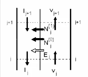
Figure 1 is a sketch of a stage or an elementary section j of an adiabatic rectifying column with vapor moving countercurrent to the falling liquid. The rates of exchange of ammonia N(1)j , water N(0)j
and energy Ej between the streams are considered
positive in the direction of vapor to liquid.
Nonequilibrium Modeling of an Ammonia-Water Rectifying Column 541
Whilst in the equilibrium stage models the balance equations are written for the whole stage or elementary section, in the nonequilibrium models the conservation equations are required for each phase within each elementary section, as presented below, starting with the molar balances for both constituents:
(1)
j 1 j 1 j j j
y+ v+ − y v + N =0 (1)
(0)
j 1 j 1 j j j
(1 y− + ) v+ − (1 y ) v− + N =0 (2)
(1)
j j j 1 j 1 j
x l − x + l+ − N =0 (3)
(0)
j j j 1 j 1 j
(1 x ) l− − (1 x− + ) l+ − N =0 (4)
The energy balances are also produced for each phase:
V V
j 1 j 1 j j j
v + h + − v h + E =0 (5)
L L
j j j 1 j j
l h − l+ h − E =0 (6)
At first sight, the equations for the mass transfer rates can be provided for both constituents in both phases, as written below:
j j 1
V
(1) I T I
j j j j
j
y y
N A y N y
2 + +
= κ ∆ − +
(7)
j j 1
L
(1) I T I
j j j j
j
x x
N A x N x
2 + +
= κ ∆ − +
(8)
j j 1
V
(0) I T I
j j j j
j
y y
N A y N (1 y )
2 + +
= κ ∆ − + −
(9)
j j 1
L
(0) I T I
j j j j
j
x x
N A x N (1 x )
2 + +
= κ ∆ − + −
(10)
The first terms on the right-hand side of equations (7) to (10) correspond to the finite difference approximation for the diffusive transport, and the last terms account for the bulk motion, which is influenced by condensation or evaporation. Either by adding equations (7) and (9) or by adding equations (8) and (10) one obtains
(0) (1) T
j
j j
N + N = N (11)
showing that equations (7) to (10) are linearly dependent. Equation (10) is not used to eliminate redundancy, and Eq. (9) is substituted by the simpler Eq. (11).
The energy balance for each phase yields
V V
j j 1
V I
j j j
(1) (1)V (0) (0)V
j j j j
T T
E A T
2
N h N h
+
+
= λ ∆ − +
+ +
(12)
L L
j j 1
L I
j j j
(1) (1)L (0) (0)L
j j j j
T T
E A T
2
N h N h
+
+
= λ ∆ − +
+ +
(13)
The first terms on the right-hand side of Eqs. (12) and (13) correspond to a finite difference approximation for the heat conduction at the interface. The other terms represent the partial enthalpy of each constituent in the mixture associated with the material fluxes through the interface.
A unique pressure pj in the elementary volume is assumed. Equilibrium conditions at the interface impose a unique temperature TjI as well as unique chemical potentials on each component in both phases:
I I
(1)L (1)V
j j
µ = µ (14)
I I
(0)L (0)V
j j
µ = µ (15)
Krishnamurthy and Taylor substitute Eqs. (14) and (15) by a relation of type I I
j j j
y =K x , obtaining
j
K by thermodynamic state equations such as
The system is completed with the relevant equations of state expressed in terms of pressure, temperature and concentration, yielding the following properties:
a) enthalpies of the liquid and the vapor bulk flows at the entrance and the exit of each elementary section:
L L L
j j j j j
h =h (T , p , x ) (16)
V V V
j j j j j
h =h (T , p , y ) (17)
b) enthalpies of each constituent in the mixture at the interface for each phase:
I
(1)L (1)L I I
j j j
j j
h =h (T , p , x ) (18)
I
(1)V (1)V I I
j j j
j j
h =h (T , p , y ) (19)
I
(0)L (0)L I I
j j j
j j
h =h (T , p , x ) (20)
I
(0)V (0)V I I
j j j
j j
h =h (T , p , y ) (21)
c) potential functions of each constituent in the mixture at the interface for each phase:
I
(1)L (1)L I I
j j j
j j (T , p , x )
µ = µ (22)
I
(1)V (1)V I I
j j j
j j (T , p , y )
µ = µ (23)
I
(0)L (0)L I I
j j j
j j (T , p , x )
µ = µ (24)
I
(0)V (0)V I I
j j j
j j (T , p , y )
µ = µ (25)
Thermodynamic Properties
The thermodynamic relations (16) to (25) are reproduced according to the method of Schulz (1972), modified by Ziegler and Trepp (1984). The method is based on two fundamental equations for Gibbs free energy in terms of temperature, pressure and concentration, one for the liquid phase,
L
g (T, p, x), and the other for the vapor, g (T, p, y)V , with the two results being equal under at saturation conditions. The liquid solution is taken to be a
nonideal mixture, so that the Gibbs free energy is the sum of the contributions of the pure components, the ideal free energy of mixing and the excess free energy:
[
]
L (0)L (1)L
E
g (1 x)g xg
RT (1 x) ln(1 x) x ln x g
= − + +
+ − − + +
(26)
The vapor mixture is assumed to be an ideal solution of non-ideal gases, so that no excess free energy is required:
[
]
V (0)V (1)V
g (1 y)g yg
RT (1 y) ln(1 y) y ln y
= − + +
+ − − +
(27)
The free energy for each component is expressed as a polynomial in terms of temperature, its inverse, and pressure, i.e., g(0)L =g (0)L(T, p) and so on
for g(1)L, g(0)V and g(1)V. The excess free energy is a polynomial on temperature, its inverse, pressure and concentration, gE = g (T, p, x)E . The relevant thermodynamic properties are obtained via the fundamental relations exemplified below for the case of the liquid.
The molar enthalpy of the mixture is given by
(
L)
L 2
p,x
g T
h T
T
∂
= −
∂
(28)
The molar chemical potential for water and ammonia in the mixture are respectively given by:
L
(0)L L
T,p g
g x
x
∂
µ = −
∂
(29)
L
(1)L L
T,p g
g (1 x)
x
∂
µ = + −
∂
(30)
The partial molar enthalpy for water and ammonia in the mixture are respectively given by (Ruiter, 1986)
L
(0)L L
T,p h
h h x
x
∂
= −
∂
Nonequilibrium Modeling of an Ammonia-Water Rectifying Column 543
L
(1)L L
T,p h
h h (1 x)
x
∂
= + −
∂
(32)
Equations analogous to (28) to (32) can be written for the vapor phase using y instead of
x
. Since the vapor mixture is considered ideal, the specific enthalpy of each component in the mixture coincides with its value as pure vapor.An alternative procedure for establishing the thermodynamic properties departs from the Helmholtz free energy put in terms of temperature, density and concentration, as presented for the ammonia-water mixture by Tillner-Roth and Friend (1998). This approach would be computationally more complex, as will be explained later.
Transport Properties
The packing surface area is computed according to Treybal (1981, Table 6.3); the mass transport coefficients and the effective transfer area employ the expression of Onda et al. (1968) and the heat transfer coefficients are calculated using above mass transfer coefficients and Chilton and Colburn’s (1934) analogy:
2 / 3 p
c . . Le
λ = β (33)
Both mass transport coefficients and the heat transfer coefficient on the vapor side use correction factors to cope with the nonvanishing mass flux at the interface (Taylor & Krishna, 1993, sections 8.2 and 11.4).
The mixture properties are generally calculated by some sort of interpolation between the respective properties of the pure substances. Reid et al. (1987) provide simple functions for the liquid viscosity and the vapor and the liquid conductivities (Tables 9-8, 10-3 and 10-5) in terms of temperature for several substances, including water and ammonia.
Most of the mixture properties were found according to estimation methods recorded by Poling et al. (2001), as follows. The viscosity of the pure vapors is given by the Chapman-Enskog relation (p.9.4) using Lennard-Jones potentials. The method of Reichenberg (pp.9.15-9.16) is used to calculate the viscosity of the vapor mixture. The diffusivity of ammonia and water vapor is estimated by Fuller and Giddings’ empirical relation (pp.11.10-11.12). In accordance with Poling et al. (p.10.32), the conductivity of the vapor mixture is estimated as the
mole fraction average of the conductivities of the pure vapors, since both their molecular sizes and their polarities are close.
The conductivity of the liquid mixture is presented in graphic form by Niebergall (1959, p.152) as the mass fraction average of the conductivities of the pure liquids.
The viscosity of the liquid mixture is also presented in graphic form by Niebergall (1959, p.151) and by the International Institute of Refrigeration, IIR (1994), for temperatures of 10o C or above. The interaction parameter Gij of the method of Grunberg and Nissan (Poling et al., 2001, pp.9.77-9.80) was adjusted to the IIR (1994) curve for viscosity against concentration for each temperature level according to the criteria of the minimum sum of the squares of the errors (Sant’ Anna, 2003), with an rms error of about 0.06 cP for the lowest temperatures, which decreases as the temperature increases. Subsequently, this parameter was expressed as a polynomial function of temperature, resulting in
2 ij
G =0.00011235 T −0.093324 T+21.459 (34)
for 283K< <T 422K. An analogous procedure for the parameter ψij of the method of Teja and Rice
(Poling et al., 2001, pp.9.85-9.87) produced higher errors for the lowest temperatures.
The surface tension was modeled according to the Macleod-Sugden correlation for the mixtures (Poling et al., 2001, p.12.12-12.16), gathering information from: a) tables 5.1 and 5.2 of the IIR (1994) publication, presenting the surface tension of each pure component for wide ranges of saturation conditions; b) graph 4.2 of the same publication, showing the surface tension of the mixture against the mass concentration for pressures 10 and 17 bar, including the pure substances as extreme cases; and c) graph 7 of ILKA Berechnungs katalog (1985), which is the most complete set of values for the mixture, plotting surface tension against mass concentration for temperatures between 20o and 140o C.
The almost parallel straight lines linking the points from tables 5.1 and 5.2 of IIR are obtained by fitting a power rule to the data relative to each fluid, resulting in
3
3.712
NH (71.85 )
σ = ∆ρ and
2
3.884
H O (53.67 )
σ = ∆ρ .
In order to use the Macleod-Sugden correlation for the mixtures, the intermediate power n=3.8 is adopted, so
that the parachors for pure ammonia and water became respectively 63.5 and 55.6 (N / m)1/ 3.8/(mol / cm )3 . The
binary interaction coefficient given by
ij 1.0 0.4x
λ = − was found to reproduce the data from ILKA between 20o C and 100o C with a relative rms error of 5%.
2 5
Difference of densities (0.01mol/cm3)
2 5 2 5
10.0
S
u
rf
ace T
ens
ion
(m
N/m)
Ammonia IIR (5.2)
Ammonia IIR (4.2)
Ammonia ILKA
Water IIR (5.1)
Water IIR (4.2)
Water ILKA
Figure 2: Correlation between surface tension and difference between liquid and vapor molar densities for ammonia and water
The theoretical basis for most of the existing prediction techniques for diffusivities in liquid mixtures is the Stokes-Einstein equation, derived from the hydrodynamics of a sphere, which yields
AB
A B
R T
D
6 r
=
π η (35)
where rA is the radius of the hypothetically spherical solute. Likewise dependence of DAB on T ηB is assumed in most empirical correlations for diffusion coefficients at infinite dilution and in the interpolating rule for the diffusivity at finite dilutions in accordance with Lefler and Cullinan (Poling et al., 2001). An analogous assumption is done in the present work.
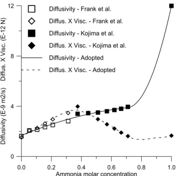
Existing experimental information on the mutual diffusivity of the liquids for different ammonia concentrations in water for 296 K is presented in Fig. 3 together with the corresponding curves for the product of diffusivity by viscosity (ηDAB). Kojima and Kashiwagi (1995) provided the diffusivity
coefficients at 296 K for seven points in the range 0.375≤ ≤x 0.71 and for the point x=1. Frank et al. (1996) gave data in the interval 0≤x≤0.312 for temperatures between 293 and 333 K ; the values used in Fig. 3 correspond to the linear interpolation between their data for 293 and 303 K after reduction to 296 K according to the dependence on viscosity and temperature indicated in (35), i.e.,
B AB
B AB
(x,T) D (x, T)
T
(x, 296)
D (x, 296)
296 η
=
η =
(36)
Almost identical results were obtained by an analogous procedure with the dependence on viscosity suggested by Frank et al. (1996) in accordance with Landolt Börnstein, i.e.,
AB B
AB B
D (x,T) (x, T)
D (x, 296) (x, 296)
η =
= η
Nonequilibrium Modeling of an Ammonia-Water Rectifying Column 545
0.0 0.2 0.4 0.6 0.8 1.0 Ammonia molar concentration
0 4 8 12
D
iffusi
vity (E
-9 m2/s) D
iffus.
X
V
is
c
. (E
-12 N
)
Diffusivity - Frank et al.
Diffus. X Visc. - Frank et al.
Diffusivity - Kojima et al.
Diffus. X Visc. - Kojima et al.
Diffusivity - Adopted
Diffus. X Visc. - Adopted
Figure 3: Diffusivity and product diffusivity by viscosity for ammonia-water mixtures at 296K.
There is a discontinuity between the two sets of results shown in Fig. 3, attributable to the different experimental methods: Kojima and Kashiwagi employed a holographic interferometric technique and Frank et al. used the Taylor-Aris dispersion method. Both results were fitted by a single second-degree polynomial with the minimum root mean square of the errors. The curve is extended to the high concentrations range by a second-degree polynomial with continuity and differentiability at x=0.71 fitted to the experimental value at x=1, resulting in the spline (38) for 296 K.
2 AB
0 x 0.71 D (x, 296) 2.565x
4.951x 1.670
≤ ≤ = − +
+ +
(38) 2
AB
0.71 x 1 D (x, 296) 91.894x
129.182x 49.2876481
≤ ≤ = −
− +
Unless otherwise stated, diffusivity is corrected for other temperatures according to (36).
Numerical Solution Method
A rectifying column composed of trays is divided into n stages, whilst a continuous contact column must be solved as a finite difference problem, as it is divided into a number of elementary volumes n
tending to infinity. The system to be solved is formed of the 23 equations (1) to (8) and (11) to (25), plus the equations for the heat and mass coefficients and for the transport properties for each elementary volume. In cocurrent devices, the equations for each volume are solved at each time, but for countercurrent devices all equations must be solved simultaneously.
The present work avoids matrices that are too huge by means of the Substitution-Newton-Raphson method (Figueiredo et al., 2002), which minimizes the order of the Newton-Raphson problem using the greatest possible number of equations in explicit or substitution fashion by choosing as effective variables those capable of fixing the greatest number of other variables. In the present problem, where the assumedly uniform pressure had been specified previously, only seven variables per elementary volume, namely vj 1+ , yj 1+ , xIj 1+ , yIj 1+ , Ti 1V+ , TiLand
I i
T , were required as effective variables The values
o
v , yo, ToV, ln, xn and TnLmust be given as boundary conditions.
The guessed or iterated values of the effective variables vj 1+ and yj 1+ allow N(1)j and ( 0 )
j
N to be
determined explicitly using Eqs. (1) and (2), and NTj using Eq. (11).
Adding Eq. (3) and (4) one obtains
(0) (1)
j j 1 j j
which allows lj to be determined sequentially from
n-1 to 0. Then the xj values are analogously determined through either Eq. (3) or (4).
In so doing, the pressure, the concentration and the temperature of each node are fixed, so that all other relevant thermodynamic properties can be computed explicitly through Eqs. (16) to (25) and
j
E , through Eq. (5). Finally, the transfer properties and coefficients are computed through the respective equations.
All the equations referred to so far – (1) to (5), (11) and (16) to (25) as well as those for the transfer properties and coefficients – were employed as substitution equations, being satisfied within the computer rounding precision and producing the substitution variables, which are not effective variables for the Newton-Raphson problem. Only the seven remaining equations for each elementary volume – (6) to (8) and (12) to (15) – constitute the residual equations to be satisfied through the Newton-Raphson procedure by varying the seven effective variables per control volume (vj 1+ , yj 1+ ,
I j 1
x + , yIj 1+ , Tj 1V+ , TjLand TjI).
The Substitution-Newton-Raphson method described above suits any Newton-Raphson algorithm, particularly those employing numerical computation of the derivatives, such as Stoecker’s Generalized System Simulation Program (1989).
Referring to the time spent on the numerical differentiation in the Newton-Raphson method, Taylor and Lucia (1995) advocated using analytical differentiation despite the complexity of the algebraic expressions of most physical properties, relying on computer algebra systems such as Mathematica or Maple. The analytical differentiation can be employed in the Substitution-Newton-Raphson method with extensive use of the chain rule to differentiate functions of functions of functions and so on. The automatic differentiation technique (Castro et al., 2000), which naturally relies on the chain rule, is another promising alternative due to its reduced computational costs and the possibility of implementation with the usual programming languages such as FORTRAN. However, the simplicity of the numerical differentiation is almost irresistible. Furthermore, by diminishing the order of the Jacobian matrix, the Substitution-Newton-Raphson method significantly reduces the computational time of the numerical differentiation in comparison with the blind Newton-Raphson method.
One can now explain the choice of computing the thermodynamic properties on the basis of the Gibbs free energy as a function of temperature, pressure and concentration, instead of using the Helmholtz free energy as a function of temperature, density and concentration. While the pressure is uniform, at least within each elementary volume, the density varies from node to node. The necessary specification of the density (or the specific volume) in the Helmholtz free energy method would increase the number of effective variables to 11 per control volume, transforming the relations between pressures at different nodes, even when equal, into residual equations.
The present code uses a residual control to minimize the risk of divergence when the initial estimates are far from the actual solution. If the total residual of an approximate solution, defined as the root mean square of the individual residuals, increases from one iteration to the next, the new solution is replaced by an intermediate estimate, which is submitted to a new residual test at most six times or until the residual diminishes; an eventual increase in the residual is accepted after six successive tests.
The physical dimensions of the effective variables are molar flow rates, temperatures and nondimensional quantities, and the dimensions of the residuals are molar flow rates, energy rates and chemical potentials. Because these dimensions are not homogeneous, the normalization of the variables and residuals is useful for adopting adequate increments in the numerical differentiation, for the stopping criteria and residual control. Estimated representative values were chosen as a normalization factor for each relevant physical dimension.
Solution of the linearized matrix employs the Gauss method with partial pivoting to minimize the risk of ill-conditioning. The Jacobian matrix of the Substitution-Newton-Raphson method is much denser than the huge matrices of the blind Newton-Raphson method, but it also becomes sparse as the number of elementary volumes n increases. To cope with that situation the present code avoids unnecessary multiplication by zero.
RESULTS
Nonequilibrium Modeling of an Ammonia-Water Rectifying Column 547
the refrigeration system and vapor emerging from the lower section of the rectifier. This lower section, called the stripping section, receives the vapor produced in the generator and the liquid that results from the mixture of the cold distillate from the upper section with the rich mixture coming from the absorber through a heat exchanger of the refrigerating system. The essential features of each section are presented at Table 1. In the present computations, the sections are treated separately.
The convergence criterium was that both the rms. of the last change in the normalized variables and the rms. of the normalized residuals should be less than
4
10− . Generally, the number of iterations required was only six for the stripping section and tem for the rectifying section, almost independently on the number of control volumes.
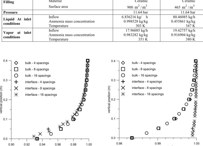
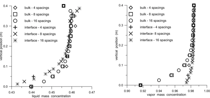
Figures 4 and 5 show the sensitivity of the bulk and interface mass concentrations for both liquid and vapor streams with respect to the grid refinement. Each section is divided into four, eight and sixteen spacings. In the rectifying section there is no noticeable difference between the results with the three levels of refinement. In the stripping section, the results with eight and sixteen spacings coincide, except for a minor difference in the liquid concentration upstream; even the results with four spacings show a small deviation from the more refined ones. There are even smaller relative differences between temperature profiles for different levels of refinement, not shown, present, so that the exit temperatures vary by only 0.1 or 0.2 K from the roughest to the finest computation.
Table 1: Rectifier specifications
Feature Rectifying
Section
Stripping Section
Length 0.4 m 0.4 m
Geometry
Diameter 0.06 m 0.1 m
Type Berl saddles ¼” Berl saddles ½”
Material Ceramic Ceramic
Filling
Surface area 900 m / m2 3 465 m / m2 3
Pressure 11.64 bar 11.64 bar
Inflow 6.836216 kg/ h 80.46085 kg/h
Ammonia mass concentration 0.998528 kg/kg 0.455861 kg/kg
Liquid At inlet conditions
Temperature 303 K 347 K
Inflow 17.96085 kg/h 19.42757 kg/h
Ammonia mass concentration 0.983282 kg/kg 0.916904 kg/kg
Vapor at inlet conditions
Temperature 351 K 380 K
0.90 0.92 0.94 0.96 0.98 1.00
liquid mass concentration
0.0 0.1 0.2 0.3 0.4
ve
rt
ica
l p
o
sitio
n
(
m
)
bulk - 4 spacings
bulk - 8 spacings
bulk - 16 spacings
interface - 4 spacings
interface - 8 spacings
interface - 16 spacings
0.98 0.99 1.00
vapor mass concentration
0.0 0.1 0.2 0.3 0.4
v
e
rt
ic
al
pos
it
ion (m)
bulk - 4 spacings
bulk - 8 spacings
bulk - 16 spacings
interface - 4 spacings
interface - 8 spacings
interface - 16 spacings
0.43 0.44 0.45 0.46 0.47 liquid mass concentration
0.0 0.1 0.2 0.3 0.4
ve
rti
c
a
l p
o
si
ti
o
n
(m)
bulk - 4 spacings
bulk - 8 spacings
bulk - 16 spacings
interface - 4 spacings
interface - 8 spacings
interface - 16 spacings
0.90 0.92 0.94 0.96 0.98 1.00 vapor mass concentration
0.0 0.1 0.2 0.3 0.4
v
e
rt
ic
al
pos
it
ion
(m
)
bulk - 4 spacings
bulk - 8 spacings
bulk - 16 spacings
interface - 4 spacings
interface- 8 spacings
interface - 16 spacings
Figure 5: Stripping section – sensitivity of concentration results to grid refinement
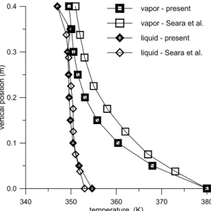
Figures 6 to 8 show comparison of the present results with those of Seara et al. (2002) and Sieves (2003) with respect to liquid and vapor mass concentrations and temperatures. The general aspects of the profiles are very similar. In both computations the interface temperature is visually coincident with the liquid temperature. The present results indicate more intensive heat and mass transfer than those of Seara et al.
They used the same representation for the thermodynamic properties of the mixture that were employed here. However, the thermodynamic modeling differed with respect to the enthalpy of the
ammonia and water crossing the interface: they employed the enthalpies and the heat of vaporization of the pure components, while the present work used the partial molar enthalpy for water and ammonia in the liquid and vapor mixtures.
The same fundamental correlations for the transport coefficients were employed in both studies except for the correction due to mass transfer through the interface: Seara et al. employed corrections for both heat transfer coefficients and for no mass transfer coefficient. The expressions for the effective transfer area differed, as well as many expressions for the transport properties.
0.92 0.94 0.96 0.98 1.00
liquid and vapor mass concentration 0.0
0.1 0.2 0.3 0.4
v
e
rt
ic
al
p
o
s
iti
on
(m
)
vapor bulk - present
vapor bulk - Seara et al.
liquid bulk - present
liquid bulk - Seara et al.
300 320 340 360
temperature (K) 0.0
0.1 0.2 0.3 0.4
v
er
ti
c
al
pos
it
io
n
(m
)
vapor - present
vapor - Seara et al.
liquid - present
liquid - Seara et al.
Nonequilibrium Modeling of an Ammonia-Water Rectifying Column 549
0.42 0.43 0.44 0.45 0.46 0.47 liquid mass concentration
0.0 0.1 0.2 0.3 0.4
v
e
rt
ic
al
pos
it
io
n
(m
)
bulk liquid - present
bulk liquid - Seara et al.
0.90 0.92 0.94 0.96 0.98 1.00 vapor mass concentration
0.0 0.1 0.2 0.3 0.4
ve
rt
ic
a
l
p
o
s
it
ion
(m
)
bulk vapor - present
bulk vapor - Seara et al.
Figure 7: Stripping section – comparison with Seara et al. results for concentrations
340 350 360 370 380
temperature (K) 0.0
0.1 0.2 0.3 0.4
v
e
rt
ic
al
po
s
it
ion
(
m
)
vapor - present
vapor - Seara et al.
liquid - present
liquid - Seara et al.
Figure 8: Stripping section – comparison with Seara et al. results for temperatures
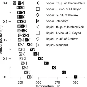
To assess the sensitivity of the results for alternative methods of computing various physical properties, one property at a time is subjected to a different calculation procedure, maintaining the remaining properties as reported previously.
In several cases no significant change in either temperature or concentration profiles was observed for both the rectifying and the stripping sections. This occurred when the gas mixture conductivity was computed in accordance with Mason and Saxena (Poling et al., 2001, p.10.31), when the gas mixture viscosity was computed in accordance with the method of Wilke (Poling et al., 2001, p.9.21-9.22) and when the liquid mixture conductivity was
computed by the method of El-Sayed as described by Thorin (2000).
No significant change was observed when the diffusivity of the liquid mixture was calculated either by extrapolation of Eq. (38) to different temperatures by means of Eq. (37) or by Nakanishi´s method for dilute solutions together with Leffler and Cullinan´s interpolation rule for finite concentrations (Poling et al., 2001, p.11.27-11.32, 11.36) and Heidemann and Rizvi´s method (1986) for thermodynamic correction.
diffusivity produced the most significant change in the concentration pattern of the rectifying section and a noticeable change in the stripping section. El-Sayed´s correlation for the viscosity of the liquid mixture, as described by Thorin (2000), produced some change in the liquid concentration profile and, primarily, in the vapor temperature profile for the rectifying section.
Ibrahim and Klein´s (1993) coefficients for the excess terms of the thermodynamic properties in Ziegler and Trepp´s method (1984) most heavily altered the liquid concentration and the temperature of the stripping section. It must be observed that in the rectifying section the ammonia concentrations are very high, so that pure ammonia properties dominate the excess terms of mixing.
0.92 0.94 0.96 0.98 1.00 liquid and vapor bulk mass concentration (kg/kg) 0.0
0.1 0.2 0.3 0.4
v
e
rt
ic
al po
s
ition
(m
)
liquid - therm. props. of Ibrahim/Klein liquid - liq. visc. of El-Sayed liquid - diffus. of Brokaw liquid - standard
vapor - therm. props. of Ibrahim/Klein vapor - liq. visc. of El-Sayed vapor - diffus. of Brokaw vapor - standard
300 320 340 360
temperature (K) 0.0
0.1 0.2 0.3 0.4
v
e
rt
ic
al
pos
it
io
n (
m
)
vapor - th. p. of Ibrahim/Klein vapor - liq. visc. of El-Sayed vapor - vap. diffus. of Brokaw vapor - standard
liquid - th. p. of Ibrahim/Klein liquid - liq. visc. of El-Sayed liquid - vap. diffus. of Brokaw liquid - standard
Figure 9: Rectifying section – sensitivity to some expressions for physical properties
0.90 0.92 0.94 0.96 0.98 1.00 bulk vapor mass concentration
0.0 0.1 0.2 0.3 0.4
v
e
rt
ic
al
pos
it
ion
(
m
)
therm. prop. of Ibrahim/Klein
liq. visc. of El-Sayed
vapor difffus. of Brokaw
standard.
0.43 0.44 0.45 0.46 0.47 bulk liquid mass concentration
0.0 0.1 0.2 0.3 0.4
v
e
rt
ic
al
pos
it
ion (
m
)
therm. p. of Ibrahim/Klein
liq. visc. of El-Sayed
vapor difffus. of Brokaw
standard.
Nonequilibrium Modeling of an Ammonia-Water Rectifying Column 551
350 360 370 380 temperature (K)
0.0 0.1 0.2 0.3 0.4
v
e
rt
ic
al
pos
it
io
n
(
m
)
vapor - th. p. of Ibrahim/Klein
vapor - l. visc. of El-Sayed
vapor - v. dif. of Brokaw
vapor - standard
liquid - th. p. of Ibrahim/Klein
liquid - l. visc. of El-Sayed
liquid - v. dif. of Brokaw
liquid - standard
Figure 11: Stripping section – sensitivity of temperature to some expressions for properties
CONCLUSION
A Newton-Raphson procedure was successfully applied to the solution of the system of equations representing the combined nonequilibrium heat and mass transfer in a packed bed rectifier. A moderate numerical grid refinement was sufficient to produce spatially converged solutions.
The uncertainties associated with the thermophysical properties were assessed by comparison between different alternative approaches. Liquid mixture viscosity and vapor diffusivity were the transport properties having the most influence on the results; important effects were also observed with an alternative procedure for the thermodynamic properties.
ACKNOWLEDGMENTS
The authors express their gratitude for the financial support provided by FINEP (Funding for Studies and Projects) under grant 21.01.04555.00.
NOMENCLATURE
Latin Symbols
A heat or mass transfer area (m2)
p
c specific heat at constant pressure
(J/kg/K)
D mass diffusivity (m2/s)
E energy flux ( W )
g molar Gibbs free energy ( J/mol )
ij
G non-dimensional parameter
in Grunberg-Nissan formula for mixture viscosity
(-)
h molar enthalpy ( J/mol )
j
K coefficient of
proportionality between the mole fractions of the liquid and the vapor in
equilibrium
(-)
l molar flux of liquid mixture ( mol/s )
Le Lewis number,
p
Le k/(= ρ c D), where k is thermal conductivity (W / m / K) and ρ is density
(kg / m3)
N component flux ( mol/s )
n number of control volumes
in distillation column
(-)
R ideal gas constant (8.314 J/(mol.K) )
A
r radius of the assumedly
spherical solute in Stokes-Einstein equation
(m)
T temperature ( K )
v molar flux of vapor mixture ( mol/s )
x ammonia molar
concentration in liquid mixture
( mol/mol )
X ammonia mass concentration
in liquid mixture
( kg/kg )
y ammonia molar concentration in vapor mixture
Greek Symbols
∆ρ difference between liquid
and vapor molar densities ( mol/ 3 cm )
η dynamic viscosity
(Ns/m2)
κ mass transfer coefficient ( mol/(sm2
mol/mol ) ) λ heat transfer coefficient ( W/(m2K) )
ij
λ binary interaction
coefficient in Macleod-Sugden correlation for mixture surface tension
(-)
µ molar chemical potential ( J/mol )
σ surface tension ( mN/m )
ij
ψ nondimensional parameter
in Teja and Rice formula for mixture viscosity
(-)
Subscripts
A relative to the solute in a mixture
(-)
B relative to the solvent in a mixture
(-)
j relative either to the j-th tray/control volume or to the boundary between (j-1)-th and j-(j-1)-th trays/control volumes in distillation column
(-)
E excess property of the mixture (increment with respect to ideal mixture)
(-)
Superscripts
(0) relative to water (-)
(1) relative to ammonia (-)
I relative to the interface (-)
L relative to the liquid phase (-)
T total (water plus ammonia) (-)
V relative to the vapor phase (-)
REFERENCES
Castro, M. C., Vieira, R. C. & Biscaia Jr., E. C. Automatic Differentiation Tools in the Dynamic Simulation of Chemical Engineering Processes Braz. J. Chem. Eng., v. 17, n. 4-7, pp. 373-382 (2000).
Chilton, T. H. & Colburn, A. P. Mass Transfer
(Absorption) Coefficients – Prediction from Data on Heat Transfer and Fluid Friction, Ind. Engng. Chem., v. 26, pp. 1183-1187 (1934).
Figueiredo, J. R., Santos, R. G., Favaro, C., Silva, A. F. S. & Sbravati, A., Substitution-Newton-Raphson Method Applied to the Modeling of a Vapour Compression Refrigeration System Using Different Representations of the Thermodynamic Properties of R-134a, J. of the Braz. Soc. Mechanical Sciences, v. XXIV, pp. 158-168 (2002).
Frank, M. J. W., Kuipers, J. A. M. & Swaaij, W. P. M. van, Diffusion Coefficients and Viscosities of
2 2
CO +H O, CO2+CH OH3 , NH3+H O2 , and
3 3
NH +CH OH Liquid Mixtures, J. Chem. Eng. Data, v. 41, pp. 297-302 (1996).
Heidemann, R. A. & Rizvi, S. S. H., Correlation of Ammonia-Water Equilibrium Data with Various Modified Peng-Robinson Equations of State, Fluid Phase Equilibria, pp. 439-446 (1986).
Ibrahim, O. M. & Klein, S. A., Thermodynamic Properties of Ammonia-Water
Mixtures, ASHRAE Transactions, 99, pp. 1495-1502 (1993).
IIR, Thermodynamic and physical properties NH3-H2O, Paris (1994).
ILKA, Berechnungs katalog, Dresden (1985).
Kojima, M. & Kashiwagi, T., Mass Diffusivity Measurements for Ammonia-Vapour Absorption Processes, 19th Int. Congress of Refrigeration, The Hague, v. IV-a, pp. 353-360 (1995).
Krishnamurthy, R. & Taylor, R., A Nonequilibrium Stage Model of Multicomponent Separation Processes – Part I: Model Description and Method of Solution, AIChE Journal, v. 31, n. 3, pp. 449-456 (1985-a).
Krishnamurthy, R. & Taylor, R., A Nonequilibrium Stage Model of Multicomponent Separation Processes – Part II: Comparison with Experiment, AIChE Journal, v. 31, n. 3, pp. 456-465 (1985-b). Krishnamurthy, R. & Taylor, R., A Nonequilibrium
Stage Model of Multicomponent Separation Processes – Part III: The Influence of Unequal Component-Efficiencies in Process Design Problems, AIChE Journal, v. 31, n. 12, pp. 1973-1985 (1973-1985-c).
Niebergall, W., Handbuch der Kaltetechnik - v. 7 Sorptions-Kältemaschinen, Springer-Verlag, Berlin (1959).
Nonequilibrium Modeling of an Ammonia-Water Rectifying Column 553
Perry, R. H. & Green, D. W., Perry´s Chemical Engineers Handbook, McGraw-Hill, New York, p. 5-75 (1997).
Poling, B. E., Prausnitz, J. M. & O’Connell, J. P., The Properties of Gases and Liquids, McGraw-Hill, New York (2001).
Raal, J. D. & Khurana, M. K., Gas Absorption with Large Heat Effects in Packed Columns, Canadian J. Chem. Eng. v. 51, pp. 162-167 (1972).
Reid, R. C., Prausnitz, J. M & Poling, B. E., The Properties of Gases and Liquids, McGraw-Hill, New York (1987).
Ruiter, J. P., Thermodynamic Description of Mixtures and Solutions, Kema Scientific & Technical Report, v. 4, n. 9 (1986).
Sant’ Anna, F. C., Experimental Evaluation of an Ammonia-Water Absorption Refrigeration/Heat Pump System (in Portuguese), Scientific Initiation Report, UNICAMP, Campinas (2003).
Schulz, S. C. G., Equations of State for the System Ammonia-Water for Use with Computers, International Congress of Refrigeration Proceedings, v. 2 pp. 431-436 (1972).
Seara, J. F., Sieres, J. & Vázques, M., Simultaneous Heat and Mass Transfer of a Packed Distillation Column for Ammonia-Water Absorption Refrigeration Systems, Intern. J. Thermal Sciences, v. 41 pp. 927-935 (2002).
Sieres, J., Escuela Técnica Superior de Ingenieros Industriales de Vigo, Spain, private communication (2003).
Stoecker, W. F., Design of Thermal Systems, Mc-Graw-Hill, New York (1989).
Taylor, R. & Krishna, R., Multicomponent Mass Transfer, John Wiley & Sons, New York (1993). Taylor, R. & Lucia, A. Modeling and Analysis of
Multicomponent Separation Processes, AIChE Symposium Series 304, v. 91, pp. 19-28 (1995). Thorin, E., On Thermophysical Properties of
Ammonia-Water Mixtures for Prediction of Heat Transfer Areas in Power Cycles, Symposium on Thermophysical Properties, June 25-30, Boulder, Colorado (2000)
Tillner-Roth, R. & Friend, D. G., A Helmholtz Free Energy Formulation of the Thermodynamic Properties of the Mixture {Water + Ammonia}, J. Phys. Chem. Ref. Data, v. 27, n. 1, pp. 63-96 (1998). Torres, L. G., Martins, F. J. D. & Bogle, I. D. L.,
Comparison of a Reduced Order Model for Packed Separation Processes and a Rigorous Non-equilibrium Stage Model, Braz. J. Chem. Eng., v. 17, n. 4-7, pp. 915-924 (2000).
Treybal, R. E., Mass Transfer Operations, McGraw-Hill, Auckland, pp. 204-205 (1981).