Geosci. Model Dev., 6, 345–352, 2013 www.geosci-model-dev.net/6/345/2013/ doi:10.5194/gmd-6-345-2013
© Author(s) 2013. CC Attribution 3.0 License.
Geoscientiic
Model Development
Open Access
Geoscientiic
Using model reduction to predict the soil-surface C
18
OO flux: an
example of representing complex biogeochemical dynamics in a
computationally efficient manner
W. J. Riley
Earth Sciences Division, Lawrence Berkeley National Laboratory, Bldg 84-1134, 1 Cyclotron Road, Berkeley, California 94720, USA
Correspondence to:W. J. Riley ([email protected])
Received: 11 September 2012 – Published in Geosci. Model Dev. Discuss.: 2 November 2012 Revised: 9 February 2013 – Accepted: 25 February 2013 – Published: 12 March 2013
Abstract.Earth system models (ESMs) must calculate large-scale interactions between the land and atmosphere while accurately characterizing fine-scale spatial heterogeneity in water, carbon, and other nutrient dynamics. We present here a high-dimension model representation (HDMR) approach that allows detailed process representation of a coupled car-bon and water tracer (theδ18O value of the soil-surface CO2 flux (δFs)) in a computationally tractable manner. δFs de-pends on theδ18O value of soil water, soil moisture and tem-perature, and soil CO2 production (all of which are depth dependent), and theδ18O value of above-surface CO2. We tested the HDMR approach over a growing season in a C4-dominated pasture using two vertical soil discretizations. The difference between the HDMR approach and the full model solution in the three-month integrated isoflux was less than 0.2 % (0.5 mol m−2‰), and the approach is up to 100 times faster than the full numerical solution. This type of model reduction approach allows representation of complex cou-pled biogeochemical processes in regional and global cli-mate models and can be extended to characterize subgrid-scale spatial heterogeneity.
1 Introduction
Atmospheric CO2 has substantial impacts on global cli-mate, both over the long term and, as we have witnessed since the beginning of the industrial revolution, much shorter timescales (Watson et al., 2001). As a result, the impacts of anthropogenic CO2emissions and climate system feedbacks
on the long-term state and stability of the climate are cur-rently the focus of much research. Since interactions with the terrestrial biosphere dominate spatial and inter- and intra-annual variations in atmospheric CO2concentrations (Tans et al., 1990), developing reliable models of ecosystem CO2 exchanges is necessary to predict future climate.
Terrestrial carbon cycle models used at the site and re-gional scales and in Earth system models (ESMs; e.g., Bo-nan et al., 2002; Denning et al., 1996; Parton et al., 1988) are based on representations of varying complexity of the biological, chemical, and physical processes governing car-bon exchanges between the atmosphere, soils, and plants. In ESMs, however, the level of process representation pos-sible is often a trade-off between the desire to mechanis-tically represent the process, ability to characterize surface and subsurface properties, and computational constraints. It is also now recognized that land models must represent some of the subgrid-scale heterogeneity known to exist at scales substantially finer than those represented in current ESMs (∼100 km resolution; King et al., 2010; Thompson et al., 2011), either explicitly or by integrating scaling rules based on mechanistic process representation.
the gross CO2fluxes comprising the net flux, i.e., the assim-ilated (photosynthetic) and respired fluxes. This partitioning is necessary since the processes controlling these fluxes spond differently to environmental forcings and therefore re-quire separate model formulations and parameterizations.
Measurements of the stable isotope18O in CO2have been proposed as a tracer to partition measured net CO2fluxes into component gross fluxes (Yakir and Wang, 1996), identify re-gional distributions of CO2 exchanges (Ciais et al., 1997a, b; Cuntz et al., 2003; Francey and Tans, 1987; Peylin et al., 1999), and investigate interactions between the C and water cycles (Buenning et al., 2012; Wingate et al., 2009). How-ever, using measurements of18O in CO2for these methods requires accurate estimation of theδ18O value of the soil-surface CO2 flux (δFs (‰)), which depends on a complex suite of interactions between the C and water cycles (Riley et al., 2002; Tans, 1998). Using this example, we illustrate here a computationally efficient approach to represent these dynamics in a manner appropriate for inclusion in regional and global models.
CO2is produced in soils by heterotrophic respiration and autotrophic root respiration. The depth distribution and mag-nitude of the soil CO2source depends on soil moisture and temperature, microbial substrate and nitrogen availability and quality, and root activity (e.g., Grant et al., 2001). Once produced, the dominant CO2transport pathway to the atmo-sphere is via diffusion through open soil pores. Although not impacting the gross CO2flux, hydration and subsequent par-titioning back into the gas phase can substantially change the δ18O value of the soil-gas CO2. Upon dissolution, CO2can exchange 18O atoms with the water, thereby acquiring the 18O composition of the water. The impact of this exchange on theδ18O value of soil water (δsw(‰)) is small, since there are orders of magnitude more H2O than CO2molecules in soil moisture. The competition between CO2 diffusion through the open pore space and dissolution into the soil water can substantially impactδFs(Miller et al., 1999; Riley, 2005).
Three classes of methods to estimate δFs have been re-ported. Several authors have hypothesized that a depth-integratedδ18O value of soil water and a constant effective kinetic fractionation factor can be used (Ciais et al., 1997a, b; Miller et al., 1999; Yakir and Wang, 1996). Tans (1998) de-veloped steady-state analytical solutions forδFs, which Stern et al. (2001) applied to study the impact of invasion fluxes on the net surface C18OO exchange. Finally, numerical mod-eling approaches have been developed to account for tran-sient conditions and gradients in theδ18O value of the vari-ous water pools impactingδFs (e.g., ISOLSM from Riley et al., 2002; and Stern et al. , 1999).
ISOLSM has been integrated into the general circulation model CCM3 (Buenning et al., 2012) to investigate the im-pact of ecosystems on theδ18O value of atmospheric CO2 (δa). However, the soil-gas diffusion and reaction submod-els in ISOLSM are computationally expensive. The high-dimension model representation (HDMR) method applied
here allows reduction of the full model to a series of look-up tables, while still characterizing second order interactions between variables important in the system. This approach substantially reduces simulation runtime (by up to a factor of 100), while still generating accurateδFspredictions.
The following sections describe the methods used in ISOLSM to predictδFs, the HDMR approach, and the spe-cific application of HDMR to estimating δFs. The HDMR model is then applied to a C4-dominated grass ecosystem as a test of the approach in a dynamic simulation. Finally, we discuss potential applications of this type of approach to representing complex biogeochemical processes and spatial heterogeneity in ESMs.
2 Methods
2.1 EstimatingδFsusing ISOLSM
ISOLSM integrates modules that simulate18O ecosystem ex-changes in H2O and CO2with the land-surface model LSM1 (Bonan, 1996). LSM1 is a “big-leaf” model that calculates internally consistent ecosystem energy, CO2, and H2O ex-changes with the atmosphere. Soil moisture, advective wa-ter fluxes, and temperature, all of which impact δsw, are calculated at user-defined depths in the soil.
The isotopic mechanisms integrated in ISOLSM are de-scribed in detail by Riley et al. (2002); the model has been ap-plied in a number of other studies of isotope and bulk C and water dynamics (Aranibar et al., 2006; Cooley et al., 2005; Henderson-Sellers et al., 2006; Lai et al., 2006; McDowell et al., 2008; Riley et al., 2003, 2008, 2009; Riley, 2005; Still et al., 2009; Torn et al., 2011). A brief description of the model follows to illustrate the nature of the interactions impacting δFs. ISOLSM solves forδswusing an explicit method with boundary conditions specified for theδ18O values of precip-itation and above-canopy vapor. Surface evaporation is cal-culated in LSM1 using a laminar soil-surface boundary layer resistance and the gradient between vapor concentrations at the soil surface and canopy air. A similar approach is taken in ISOLSM to compute the soil-surface H218O flux. In this case, though, the additional effects of an equilibrium parti-tioning factor and a different laminar boundary layer resis-tance for the heavier isotopologue are included. Root wa-ter withdrawal from the soil profile (driven by transpiration) is calculated using modules from LSM1; root H218O with-drawal occurs without isotopic fractionation. In this paper, δsw is presented relative to Vienna Standard Mean Ocean Water (V-SMOW).
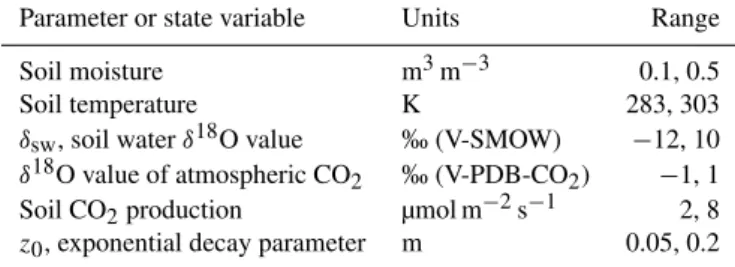
Table 1.Parameters and state variables used to generate the expan-sion functions. Spatial discretization scenarios D1 and D2 corre-spond to eight 2.5 cm and four 5 cm control volumes, respectively, in the top 20 cm of soil. All HDMR simulations are performed by dividing each parameter range into 100 equal spaces (i.e.,N=100).
Parameter or state variable Units Range
Soil moisture m3m−3 0.1, 0.5
Soil temperature K 283, 303
δsw, soil waterδ18O value ‰ (V-SMOW) −12, 10
δ18O value of atmospheric CO2 ‰ (V-PDB-CO2) −1, 1 Soil CO2production µmol m−2s−1 2, 8 z0, exponential decay parameter m 0.05, 0.2
Fs18, respectively (µmol m−2s−1)) are computed from the concentration gradients and diffusivities at the soil surface. Finally, theδ18O value of the soil-surface CO2flux is calcu-lated as
δFs18= F
18 s /Fs
rpdb
−1
!
1000, (1)
whererpdbis the Vienna Pee Dee Belemnite (V-PDB-CO2) standard. As applied here, ISOLSM uses 2.5 cm control vol-umes to solve forδsw and twenty unevenly spaced control volumes down to 1 m depth for the soil-gas calculations. Model testing is described in Riley et al. (2003), and an ap-plication of ISOLSM to analyze the impact of near-surface δswonδFsis presented in Riley (2005).
2.2 High-dimensional model reduction
The HDMR technique described here (termed the cut-HDMR) is a special application of a group of tools de-signed to represent high-dimensional models (Alis and Rab-itz, 2001; Rabitz and Alis, 1999; Rabitz et al., 1999). HDMR was developed to substantially decrease simulation runtime while retaining nonlinear interactions between state variables and model parameters. Besides cut-HDMR, other versions of the HDMR approach have been applied to environmen-tal modeling problems, e.g., random sampling HDMR (Li et al., 2006; Wang et al., 2003). The method has also been integrated with neural network approaches for high dimen-sionality problems (e.g., Manzhos and Carrington, 2008). The HDMR method has been used, for example, to study global atmospheric chemistry (Wang et al., 1999), strato-spheric chemistry (Shorter et al., 1999), and atmostrato-spheric ra-diation transport (Shorter et al., 2000).
The HDMR approach maps a set of n input variables x=(x1, x2, . . ., xn) onto the desired output g (x). In the
case of estimatingδFs, the full set of input variablesxi are
soil moisture, temperature, CO2production, andδsw(all of which are depth dependent), and the δ18O value of atmo-spheric CO2 (Table 1).g (x)representsδFs at a particular
x and is expressed as an expansion of correlated functions (f0, fi(xi) , fij xi, xj, etc.):
g (x)=f0+
n X
i=1
fi(xi)+ n X
1≤i<j≤n
fij xi, xj+. . .
+f12,...,n(x1, x2, . . ., xn) . (2)
Here,f0is a constant that represents the system response ata (i.e.,g (a)), whereais the reference point (the central point of the n-dimensional hypercube defined byx);fi(xi)
char-acterizes the impact ong (x)of a change inxi, while other
inputs are taken from the reference pointa;fij xi, xj
char-acterizes the impact ong (x)of simultaneous changes inxi
andxj; andf12...n(x1, x2, . . ., xn)gives the residual impact
ong (x)of all the variables simultaneously. The cut-HDMR approach ignores functions with greater than two variable in-teractions under the hypothesis that first and second order interactions dominateδFs. The three expansion functions are calculated as
f0=g (a) , (3)
fi(xi)=g (xi,a)−g (a) , (4)
and
fij xi, xj=g xi, xj,a−fi(xi)−fj xj−f0. (5)
The nomenclature forgindicates that it is evaluated assum-ing all variables are at the reference pointaexcept the spe-cific value(s) of x contained in the parentheses. Subtract-ing off the lower-order expansion functions when calculatSubtract-ing fij xi, xjensures a unique addition fromg xi, xj,a. 2.3 Applying HDMR to calculateδFs
For this work the HDMR expansion functions were gener-ated using ISOLSM to evaluateδFsat steady state for a suite of input variables. In general, the soil-gas system will not be in steady state, but as demonstrated below, excursions from the steady-state solution do not appreciably impact the pre-dicted cumulative isoflux in this system. The impact and ap-plicability of the steady-state assumption in different ecosys-tems and under different meteorological forcing will be eval-uated in future work. Note that the HDMR method has also been used to propagate transient solutions of complex mod-els (e.g., Shorter et al., 2000).
16
Fig. 1.Simulatedδswin four soil layers over a twenty-day period in June 2000. Spikes inδswin the top 2.5 cm result from soil evapora-tion, precipitaevapora-tion, and wicking from lower soil layers.
To develop the HDMR expansion functions, ISOLSM is run to steady state for each set of conditions (i.e., eachx). δFsis then evaluated, and the expansion functions are calcu-lated with Eqs. (3)–(5) and stored as look-up tables. Comput-ing the expansion functions for each discretization took about seven days on a 2 GHz Atherton PC with 512 MB of RAM. During the HDMR simulation, first and second order inter-polation routines are used to calculate the expansion func-tions for a specific input setx. The advantage to the HDMR approach is the ability to rapidly evaluate Eq. (2) once the expansion functions have been computed.
In ISOLSM the soil CO2source term is calculated as the sum of autotrophic and heterotrophic respiration, each with their own exponentially decaying depth profile defined by the parametersza0andzh0(m), respectively.za0andzh0are sensi-tive to soil moisture, becoming larger as the soil dries (i.e., the relative distribution of soil CO2production moves deeper as the soil dries). To save computational time, the HDMR ex-pansion functions were generated with a single exponential parameter,z0. Therefore, in the simulations presented here, the HDMR model applies a parameter weighted by the pre-dicted autotrophic,Fa(µmol m−2s−1), and heterotrophic,Fh (µmol m−2s−1), CO2sources to approximate the depth dis-tribution of CO2production:
z0=z
a 0Fa+z
h 0Fvh Fa+Fh
. (6)
2.4 HDMR testing
The HDMR approach was tested using meteorological data from May–July 2000 in a C4-dominated tallgrass prairie pas-ture in Oklahoma (36◦56′N, 96◦41′W). This dataset was
used previously to develop and test ISOLSM (Riley et al., 2002, 2003). The site is in a region with various land uses, in-cluding crops, sparse trees, and other grasslands, has not been grazed since 1996, and is burned every spring. Maximum leaf area index is about 3, and maximum net ecosystem exchange during the growing season is about 35 µmol m−2s−1. The site
17
Fig. 2.SimulatedδFsover the growing season from ISOLSM and the HDMR approach using discretization scenarios D1 and D2. Variability inδFs is large when δsw variability in the top 2.5 or 5 cm is large.
and collection of meteorological forcing and flux data are de-scribed in detail in Suyker and Verma (2001) and Colello et al. (1998).
3 Results and discussion
The magnitude and vertical distribution ofδswis an impor-tant determinant ofδFs(Riley, 2005). In this system, low hu-midity, high air temperatures, and high soil evaporation rates generate strongδswgradients in the top 5 cm of soil, making accurate prediction ofδswcritical for predictingδFs. For ex-ample, Fig. 1 shows predictedδswfor four soil layers over a twenty-day period in June 2000.
The spikes inδswin the first soil layer occur for a num-ber of reasons. Rapid increases inδsw are typically driven by large soil evaporative fluxes, which occur when the vapor gradient between the soil surface and canopy air is large. The δ18O value of above-canopy vapor (δv)is impacted by sur-face evaporative fluxes, resulting in a feedback betweenδv and near-surfaceδsw. Because we lack continuous measure-ments ofδv, we estimated it using a constant offset (7 ‰) from the estimated stem waterδ18O value. In reality,δvcan change more rapidly than this approach allows, as shown in Helliker et al. (2002). Rapid decreases inδsw are caused by precipitation inputs; wicking of more depleted soil water from lower soil layers drives more gradual decreases.
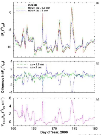
The HDMR approach using both vertical discretizations (D1 and D2) accurately simulated δFs over the growing season (Fig. 2). Figure 3 again compares the HDMR and ISOLSM predictions, but over a twenty-day period so that details inδFscan be more easily seen. Also shown in Fig. 3 is the gradient inδswover the top 5 cm of soil (∇0−5 cmδsw (‰ cm−1)).
18
Fig. 3. (a)Same as in Fig. 2, but for a 20-day period. Also shown are(b)differences between the full ISOLSM model results and the HDMR predictions for1z=2.5 and 5 cm and(c)∇0−5cmδsw, the predicted gradient inδswover the top 5 cm of soil. Differences be-tween scenarios D1and D2are largest when near-surfaceδsw gradi-ents are large. Discretization scenario D1more accurately predicts the impact of these gradients onδFssince this HDMR solution is based on the identical spatial discretization as that of the ISOLSM simulation (i.e., 2.5 cm in the top 20 cm of soil).
δswgradients between 0 and 5 cm depth. We have previously shown that these gradients can substantially impactδFs (Ri-ley, 2005). Following precipitation (e.g., days 162, 163, 164, 167, 172, and 174; Fig. 3), the enhanced soil-surface evapo-ration leads to∇0−5 cmδswof up to 5 ‰ cm−1. We have
ob-served gradients of this magnitude in a sorghum field in Ok-lahoma (unpublished data), as have Miller et al. (1999) in their soil column experiments. The impact of these gradients onδFs is better captured in scenario D1since this HDMR solution is based on the identical spatial discretization as that of the ISOLSM simulation (i.e., eight 2.5 cm control volumes in the top 20 cm of soil). Second, even in the absence of ver-tical spatial gradients inδsw, rapid changes inδswwill lead to errors in the HDMR predictions since the HDMR solution is based on the steady-state full model solution. However, the errors between the D1discretization scenario predictions and the ISOLSM solution are small during these periods of rapid change. These results imply that errors associated with
19
Fig. 4.Cumulative soil-surface isoflux calculated with ISOLSM and the HDMR approach using discretization scenarios D1and D2. The error in cumulative isoflux over the season for each HDMR scenario is about 0.2 % (0.5 mol m−2‰).
the steady-state assumption are relatively small for the con-ditions simulated here. Third, using an approximation forz0 (Eq. 2.4) will lead to errors in the depth distribution of CO2 production, although the total production will be correct. Fi-nally, the HDMR solution is linearly interpolated between the forcing values shown in Table 1; this interpolation will lead to some error. I have attempted to minimize this type of error by using relatively small increments between succes-sive values at which the expansion functions were evaluated (i.e.,N=100).
The net impact of soil-surface CO2 fluxes on the δ18O value of atmospheric CO2is described by the instantaneous isoflux,I (µmol m−2s−1‰), calculated as
I=(δFs−δa) Fs. (7)
The cumulative isoflux,Ic(mol m−2‰), is calculated as the time integral ofI over the three-month period. Ic is accu-rately simulated by the HDMR approach for both discretiza-tion scenarios (Fig. 4). Differences in the HDMR model predictions from the full model solution during periods of large near-surfaceδswgradients did not substantially impact predictions of the cumulative isoflux over the three-month period. The error in cumulative isoflux after three months is about 0.2 % (0.5 mol m−2‰) for both discretization sce-narios. The HDMR solution was computed ∼50 and 100 times faster than the full ISOLSM numerical solution for dis-cretization scenarios D1and D2, respectively. This increased computational efficiency makes it practical to include the ISOLSM-based HDMR solution for δFs in regional- and global-scale models.
others (Kleber et al., 2011). The microbial community acting at these scales is incredibly diverse (Goldfarb et al., 2011) as are the range of organic molecules being transformed and consumed (Kogel-Knabner, 2002; Sutton and Sposito, 2005). At the mm to cm scale, aggregation, macropores, plant roots, and other soil structural properties impact distributions of mi-crobes and resources (Six et al., 2001). Vertical structure of hydrology and C inputs can vary on horizontal scales as small as a few meters and vertical scales on the order of 10 cm. Ac-counting for these types of heterogeneity across 10s of km in an ESM is a substantial challenge that high-dimensional model reduction techniques such as that presented here may help address.
4 Conclusions
Representing complex coupled hydrological and biogeo-chemical processes in an Earth system model may, depend-ing on the level of mechanistic detail desired, require some level of model reduction to make the problem computation-ally feasible. We described here a high-dimensional model reduction approach to address one example of such a prob-lem – estimating the δ18O value of the soil-surface CO2 flux. This flux is a complex function of the depth-dependent (a)δ18O value of soil water, (b) soil moisture, (c) soil temper-ature, and (d) soil CO2production, as well as theδ18O value of above-surface CO2. Mechanistic models that include these interactions (e.g., ISOLSM) may be too computationally ex-pensive to integrate in regional and global models at their native spatial scale. The results presented here demonstrate that the HDMR technique accurately predictsδFs up to 100 times faster than the full numerical solution.
Under rapidly changing soil moisture conditions, such as immediately after a precipitation event, the full numerical so-lution of the C18OO surface flux differs slightly from the HDMR solution. Errors in the HDMR solution arise from the steady-state assumption, approximation of the depth de-pendence of soil CO2 production, and linear interpolation. However, these errors have a small impact on the predicted cumulative isoflux. The error in the cumulative isoflux over the growing season calculated with HDMR (compared to that calculated with the full model) was less than 0.2 %.
Applying measurements of theδ18O value of atmospheric CO2 to partition measured net ecosystem fluxes into gross fluxes and, at the regional and global scale, to estimate spa-tially explicit CO2exchanges requires accurate prediction of theδ18O value of the soil-surface CO2flux. Further, for re-gional and global simulations such a method must be compu-tationally efficient. The HDMR method applied here shows great promise as a tool for addressing the need for mechanis-tic representation of processes across a wide range of scales and spatial heterogeneity.
Nomenclature
a HDMR reference point
f0 System response ata
fi(xi) Impact ong (x)of a change inxi
fij xi, xj Impact on g (x) of simultaneous
changes inxi andxj
f12...n
(x1, x2, . . ., xn)
Residual impact ong (x)of all the variables simultaneously
Fa,Fh Autotrophic and heterotrophic CO2 sources (µmol m−2s−1)
Fs18, Fs Net soil-surface C18OO and CO2 fluxes (µmol m−2s−1)
g (x) Calculated HDMR result I Isoflux (µmol m−2s−1‰ ) Ic Cumulative isoflux (mol m−2‰ ) n Number of input variables in the
HDMR solution
N Number of intervals in the HDMR
solution for each input variable
rpdb V-PDB-CO2standard
x Vector of variables for the HDMR solution
xi Input variables for the HDMR
solution
z0 Single exponential depth profile parameter (m)
za0, zh0 Autotrophic and heterotrophic depth profile parameters (m) Greek letters
δFs δ18O value of the soil-surface CO2 flux (‰)
δsw δ18O value of soil water (‰)
∇0−5cmδsw Gradient inδswover the top 5 cm of
soil (‰ cm1)
Acknowledgements. This research was supported by the Director, Office of Science, Office of Biological and Environmental Research of the US Department of Energy under Contract No. DE-AC02-05CH11231 as part of their NGEE Arctic and ARM Programs.
References
Alis, O. F. and Rabitz, H.: Efficient implementation of high di-mensional model representations, J. Math. Chem., 29, 127–142, 2001.
Aranibar, J. N., Berry, J. A., Riley, W. J., Pataki, D. E., Law, B. E., and Ehleringer, J. R.: Combining meteorology, eddy fluxes, isotope measurements, and modeling to understand environmen-tal controls of carbon isotope discrimination at the canopy scale, Global Change Biol., 12, 710–730, 2006.
Aubinet, M., Grelle, A., Ibrom, A., Rannik, U., Moncrieff, J., Fo-ken, T., Kowalski, A. S., Martin, P. H., Berbigier, P., Bernhofer, C., Clement, R., Elbers, J., Granier, A., Grunwald, T., Morgen-stern, K., Pilegaard, K., Rebmann, C., Snijders, W., Valentini, R., Vesala, T., and Figures, P.: Estimates of the annual net carbon and water exchange of forests: The EUROFLUX methodology, Adv. Ecol. Res., 30, 113–175, 2000.
Baldocchi, D. D.: Assessing the eddy covariance technique for evaluating carbon dioxide exchange rates of ecosystems: past, present and future, Global Change Biol., 9, 479–492, 2003. Baldocchi, D., Falge, E., Gu, L. H., Olson, R., Hollinger, D.,
Running, S., Anthoni, P., Bernhofer, C., Davis, K., Evans, R., Fuentes, J., Goldstein, A., Katul, G., Law, B., Lee, X. H., Malhi, Y., Meyers, T., Munger, W., Oechel, W., Paw U, K. T., Pilegaard, K., Schmid, H. P., Valentini, R., Verma, S., Vesala, T., Wilson, K., and Wofsy, S.: FLUXNET: A new tool to study the tempo-ral and spatial variability of ecosystem-scale carbon dioxide, wa-ter vapor, and energy flux densities, B. Am. Meteorol. Soc., 82, 2415–2434, 2001.
Bonan, G. B.: A land surface model (LSM version 1.0) for ecologi-cal, hydrologiecologi-cal, and atmospheric studies: Technical description and user’s guide, 150 pp., NCAR, Boulder, CO, 1996.
Bonan, G. B., Oleson, K. W., Vertenstein, M., Levis, S., Zeng, X. B., Dai, Y. J., Dickinson, R. E., and Yang, Z. L.: The land surface climatology of the community land model coupled to the NCAR community climate model, J. Climate, 15, 3123–3149, 2002. Buenning, N., Noone, D. C., Randerson, J. T., Riley, W. J., and
Still, C. J.: The response of the 18O content of atmospheric CO2to changes in environmental conditions, J. Geophys. Res.-Biogeosci., in review, 2012.
Ciais, P., Denning, A. S., Tans, P. P., Berry, J. A., Randall, D. A., Collatz, G. J., Sellers, P. J., White, J. W. C., Trolier, M., Meijer, H. A. J., Francey, R. J., Monfray, P., and Heimann, M.: A three-dimensional synthesis study of delta O−18 in atmospheric CO2 .1. Surface fluxes, J. Geophys. Res.-Atmos., 102, 5857–5872, 1997a.
Ciais, P., Tans, P. P., Denning, A. S., Francey, R. J., Trolier, M., Meijer, H. A. J., White, J. W. C., Berry, J. A., Randall, D. A., Collatz, G. J., Sellers, P. J., Monfray, P., and Heimann, M.: A three-dimensional synthesis study of delta O−18in atmospheric CO2.2. Simulations with the TM2 transport model, J. Geophys. Res.-Atmos., 102, 5873–5883, 1997b.
Colello, G. D., Grivet, C., Sellers, P. J., and Berry, J. A.: Modeling of energy, water, and CO2flux in a temperate grassland ecosystem with SiB2: May–October 1987, J. Atmos. Sci., 55, 1141–1169, 1998.
Cooley, H. S., Riley, W. J., Torn, M. S., and He, Y.: Impact of agricultural practice on regional climate in a coupled land sur-face mesoscale model, J. Geophys. Res.-Atmos., 110, D03113, doi:10.1029/2004jd005160, 2005.
Cuntz, M., Ciais, P., Hoffmann, G., Allison, C. E., Francey, R. J., Knorr, W., Tans, P. P., White, J. W. C., and Levin, I.: A com-prehensive global three-dimensional model of delta O−18in at-mospheric CO2: 2. Mapping the atmospheric signal, J. Geophys. Res.-Atmos., 108, 2003.
Denning, A. S., Collatz, G. J., Zhang, C. G., Randall, D. A., Berry, J. A., Sellers, P. J., Colello, G. D., and Dazlich, D. A.: Simula-tions of Terrestrial Carbon Metabolism and Atmospheric CO2in a General Circulation Model .1. Surface Carbon Fluxes, Tellus B, 48, 521–542, 1996.
Francey, R. J. and Tans, P. P.: Latitudinal variation in oxygen-18 of atmospheric CO2, Nature, 327, 495–497, 1987.
Goldfarb, K. C., Karaoz, U., Hanson, C. A., Santee, C. A., Brad-ford, M. A., Treseder, K. K., Wallenstein, M. D., and Brodie, E. L.: Differential growth responses of soil bacterial taxa to carbon substrates of varying chemical recalcitrance, Frontiers in Micro-biology, 2, 94, doi:10.3389/fmicb.2011.00094, 2011.
Goulden, M. L., Munger, J. W., Fan, S. M., Daube, B. C., and Wofsy, S. C.: Measurements of Carbon Sequestration by Long-Term Eddy Covariance – Methods and a Critical Evaluation of Accuracy, Global Change Biol., 2, 169–182, 1996.
Grant, R. F., Jarvis, P. G., Massheder, J. M., Hale, S. E., Moncrieff, J. B., Rayment, M., Scott, S. L., and Berry, J. A.: Controls on carbon and energy exchange by a black spruce – moss ecosys-tem: Testing the mathematical model Ecosys with data from the BOREAS experiment, Global Biogeochem. Cy., 15, 129–147, 2001.
Helliker, B. R., Roden, J. S., Cook, C., and Ehleringer, J. R.: A rapid and precise method for sampling and determining the oxy-gen isotope ratio of atmospheric water vapor, Rapid Commun. Mass. Sp., 16, 929–932, 2002.
Henderson-Sellers, A., Fischer, M., Aleinov, I., McGuffie, K., Ri-ley, W. J., Schmidt, G. A., Sturm, K., Yoshimura, K., and Iran-nejad, P.: Stable water isotope simulation by current land-surface schemes: Results of iPILPS Phase 1, Global Planet. Change, 51, 34–58, 2006.
King, A. J., Freeman, K. R., McCormick, K. F., Lynch, R. C., Lozupone, C., Knight, R., and Schmidt, S. K.: Biogeography and habitat modelling of high-alpine bacteria, Nat. Commun., 1, 53, doi:10.1038/Ncomms1055, 2010.
Kleber, M., Nico, P. S., Plante, A. F., Filley, T., Kramer, M., Swanston, C., and Sollins, P.: Old and stable soil organic matter is not necessarily chemically recalcitrant: implications for mod-eling concepts and temperature sensitivity, Global Change Biol., 17, 1097–1107, 2011.
Kogel-Knabner, I.: The macromolecular organic composition of plant and microbial residues as inputs to soil organic matter, Soil Biol. Biochem., 34, 139–162, 2002.
Lai, C. T., Riley, W., Owensby, C., Ham, J., Schauer, A., and Ehleringer, J. R.: Seasonal and interannual variations of car-bon and oxygen isotopes of respired CO2in a tallgrass prairie: Measurements and modeling results from 3 years with contrast-ing water availability, J. Geophys. Res.-Atmos., 111, D08s06, doi:10.1029/2005jd006436, 2006.
Manzhos, S. and Carrington, T.: Using neural networks, optimized coordinates, and high-dimensional model representations to ob-tain a vinyl bromide potential surface, J. Chem. Phys., 129, 224104, doi:10.1063/1.3021471, 2008.
McDowell, N., Baldocchi, D., Barbour, M., Bickford, C., Cuntz, M., Hanson, D., Knohl, A., Powers, H., Rahn, T., Randerson, J., Riley, W., Still, C., Tu, K., and Walcroft, A.: Understand-ing the stable isotope composition of biosphere atmosphere CO2 exchange, EOS Transactions American Geophysical Union, 89, 94–95, 2008.
Miller, J. B., Yakir, D., White, J. W. C., and Tans, P. P.: Measure-ment of O−18/O−16 in the soil-atmosphere CO2 flux, Global Biogeochem. Cy., 13, 761–774, 1999.
Parton, W. J., Mosier, A. R., and Schimel, D. S.: Dynamics of C, N, P, and S in grassland soils: a model, Biogeochemistry, 5, 109– 131, 1988.
Peylin, P., Ciais, P., Denning, A. S., Tans, P. P., Berry, J. A., and White, J. W. C.: A 3-dimensional study of delta O−18in atmo-spheric CO2: contribution of different land ecosystems, Tellus B, 51, 642–667, 1999.
Rabitz, H. and Alis, O. F.: General foundations of high-dimensional model representations, J. Math. Chem., 25, 197–233, 1999. Rabitz, H., Alis, O. F., Shorter, J., and Shim, K.: Efficient
input-output model representations, Comput. Phys. Commun., 117, 11–20, 1999.
Riley, W. J.: A modeling study of the impact of the delta O−18value of near-surface soil water on the delta O−18 value of the soil-surface CO2flux, Geochim. Cosmochim. Ac., 69, 1939–1946, 2005.
Riley, W., Still, C., Torn, M., and Berry, J.: A mechanistic model of H182 O and C18OO fluxes between ecosystems and the atmo-sphere: Model description and sensitivity analyses, Global Bio-geochem. Cy., 16, 1095–1109, 2002.
Riley, W. J., Still, C. J., Helliker, B. R., Ribas-Carbo, M., and Berry, J. A.:18O composition of CO2and H2O ecosystem pools and fluxes in a tallgrass prairie: Simulations and comparisons to mea-surements, Global Change Biol., 9, 1567–1581, 2003.
Riley, W. J., Hsueh, D. Y., Randerson, J. T., Fischer, M. L., Hatch, J. G., Pataki, D. E., Wang, W., and Goulden, M. L.: Where do fossil fuel carbon dioxide emissions from California go? An analysis based on radiocarbon observations and an atmospheric transport model, J. Geophys. Res.-Biogeosci., 113, G04002, doi:10.1029/2007jg000625, 2008.
Riley, W. J., Biraud, S. C., Torn, M. S., Fischer, M. L., Billes-bach, D. P., and Berry, J. A.: Regional CO2and latent heat sur-face fluxes in the Southern Great Plains: Measurements, mod-eling, and scaling, J. Geophys. Res.-Biogeosci., 114, G04009, doi:10.1029/2009jg001003, 2009.
Shorter, J. A., Ip, P. C., and Rabitz, H. A.: An efficient chemical kinetics solver using high dimensional model representation, J. Phys. Chem., 103, 7192–7198, 1999.
Shorter, J., Ip, P., and Rabitz, H.: Radiation transport simulation by means of a fully equivalent operational model, Geophys. Res. Lett., 27, 3485–3488, 2000.
Six, J., Guggenberger, G., Paustian, K., Haumaier, L., Elliott, E. T., and Zech, W.: Sources and composition of soil organic matter fractions between and within soil aggregates, Eur. J. Soil Sci., 52, 607–618, 2001.
Stern, L. A., Baisden, W. T., and Amundson, R.: Processes control-ling the oxygen isotope ratio of soil CO2: Analytic and numerical modeling, Geochim. Cosmochim. Ac., 63, 799–814, 1999. Stern, L. A., Amundson, R., and Baisden, W. T.: Influence of
soils on oxygen isotope ratio of atmospheric CO2, Global Bio-geochem. Cy., 15, 753–759, 2001.
Still, C. J., Riley, W. J., Biraud, S. C., Noone, D. C., Buenning, N. H., Randerson, J. T., Torn, M. S., Welker, J., White, J. W. C., Vachon, R., Farquhar, G. D., and Berry, J. A.: Influence of clouds and diffuse radiation on ecosystem-atmosphere CO2 and (COO)-O−18exchanges, J. Geophys. Res.-Biogeosci., 114, G01018, doi:10.1029/2007jg000675, 2009.
Sutton, R. and Sposito, G.: Molecular structure in soil humic sub-stances: The new view, Environ. Sci. Technol., 39, 9009–9015, 2005.
Suyker, A. E. and Verma, S. B.: Year-round observations of the net ecosystem exchange of carbon dioxide in a native tallgrass prairie, Global Change Biol., 7, 279–289, 2001.
Tans, P. P.: Oxygen isotopic equilibrium between carbon dioxide and water in soils, Tellus B, 50, 163–178, 1998.
Tans, P., Fung, I., and Takahashi, T.: Observational constraints on the global atmospheric carbon dioxide budget, Science, 247, 1431–1443, 1990.
Thompson, S. E., Harman, C. J., Troch, P. A., Brooks, P. D., and Sivapalan, M.: Spatial scale dependence of ecohydrologically mediated water balance partitioning: A synthesis framework for catchment ecohydrology, Water Resour. Res., 47, W00j03, doi:10.1029/2010wr009998, 2011.
Torn, M. S., Biraud, S. C., Still, C. J., Riley, W. J., and Berry, J. A.: Seasonal and interannual variability in C−13composition of ecosystem carbon fluxes in the US Southern Great Plains, Tellus B, 63, 181–195, 2011.
Wang, S. W., Levy, H., Li, G., and Rabitz, H.: Fully equivalent operational models for atmospheric chemical kinetics within global chemistry-transport models, J. Geophys. Res.-Atmos., 104, 30417–30426, 1999.
Wang, S. W., Georgopoulos, P. G., Li, G. Y., and Rabitz, H.: Random sampling-high dimensional model representation (RS-HDMR) with nonuniformly distributed variables: Application to an integrated multimedia/multipathway exposure and dose model for trichloroethylene, J. Phys. Chem. A, 107, 4707–4716, 2003.
Watson, R. T. and Albritton, D. L.: Intergovernmental Panel on mate Change. Working Group I, Intergovernmental Panel on Cli-mate Change. Working Group II, and Intergovernmental Panel on Climate Change. Working Group III, Climate Change 2001: synthesis report, x, 397 pp., Cambridge University Press, Cam-bridge, New York, 2001.
Wingate, L., Ogee, J., Cuntz, M., Genty, B., Reiter, I., Seibt, U., Yakir, D., Maseyk, K., Pendall, E. G., Barbour, M. M., Mor-tazavi, B., Burlett, R., Peylin, P., Miller, J., Mencuccini, M., Shim, J. H., Hunt, J., and Grace, J.: The impact of soil microor-ganisms on the global budget of delta O−18in atmospheric CO2, Proc. Natl. Acad. Sci. USA, 106, 22411–22415, 2009.