www.atmos-chem-phys.net/6/4867/2006/ © Author(s) 2006. This work is licensed under a Creative Commons License.
Chemistry
and Physics
Implementation of a Markov Chain Monte Carlo method to
inorganic aerosol modeling of observations from the MCMA-2003
campaign – Part I: Model description and application to the La
Merced site
F. M. San Martini1,*, E. J. Dunlea1,**, M. Grutter2, T. B. Onasch3, J. T. Jayne3, M. R. Canagaratna3, D. R. Worsnop3, C. E. Kolb3, J. H. Shorter3, S. C. Herndon3, M. S. Zahniser3, J. M. Ortega1,***, G. J. McRae4, L. T. Molina1,5, and M. J. Molina1,6
1Department of Earth, Atmospheric, and Planetary Sciences, Massachusetts Institute of Technology, Cambridge, MA, USA 2Centro de Ciencias de la Atm´osfera, Universidad Nacional Aut´onoma de M´exico, Mexico City, Mexico
3Aerodyne Research Inc., Billerica, MA, USA
4Department of Chemical Engineering, Massachusetts Institute of Technology, Cambridge, MA, USA 5Molina Center on Energy and the Environment, La Jolla, CA, USA
6Department of Chemistry and Biochemistry, University of California, San Diego, CA, USA
*now at: the Board on Chemical Sciences and Technology, National Academies, Washington, D.C., USA
**Cooperative Institute for Research in the Environmental Sciences (CIRES), Univ. of Colorado at Boulder, Boulder, CO,
USA
***now at: Sandia National Laboratory, Livermore, CA, USA
Received: 9 May 2006 – Published in Atmos. Chem. Phys. Discuss.: 10 July 2006 Revised: 16 October 2006 – Accepted: 24 October 2006 – Published: 30 October 2006
Abstract. The equilibrium inorganic aerosol model
ISOR-ROPIA was embedded in a Markov Chain Monte Carlo al-gorithm to develop a powerful tool to analyze aerosol data and predict gas phase concentrations where these are unavail-able. The method directly incorporates measurement uncer-tainty, prior knowledge, and provides a formal framework to combine measurements of different quality. The method was applied to particle- and gas-phase precursor observations taken at La Merced during the Mexico City Metropolitan Area (MCMA) 2003 Field Campaign and served to discrim-inate between diverging gas-phase observations of ammonia and predict gas-phase concentrations of hydrochloric acid. The model reproduced observations of particle-phase ammo-nium, nitrate, and sulfate well. The most likely concentra-tions of ammonia were found to vary between 4 and 26 ppbv, while the range for nitric acid was 0.1 to 55 ppbv. During periods where the aerosol chloride observations were consis-tently above the detection limit, the model was able to repro-duce the aerosol chloride observations well and predicted the most likely gas-phase hydrochloric acid concentration var-ied between 0.4 and 5 ppbv. Despite the high ammonia con-Correspondence to:F. M. San Martini
centrations observed and predicted by the model, when the aerosols were assumed to be in the efflorescence branch they are predicted to be acidic (pH∼3).
1 Introduction
Mexico City has long been well-known for its poor air quality (Molina and Molina, 2002). The 2003 Mexico City Metropolitan Area (MCMA) field campaign was an inten-sive 5-week campaign focused on providing a scientific base for devising emissions control strategies to reduce exposure to harmful pollutants in the MCMA, as well as insights to air pollution problems in other megacities. In this paper we use data from the MCMA-2003 campaign to illustrate the application of a Bayesian method to infer missing and un-certain measurements, focusing on the inorganic aerosol sys-tem. We focus on the inorganic aerosols because the health risk of air pollution in the MCMA is dominated by the ef-fect of particles (Evans et al., 2002), and, although organic aerosols comprise a majority of the fine particle mass in the MCMA, uncertainties in both modeling (Ansari and Pandis, 2000b; Clegg et al., 2001, 2003) and measurements (Mc-Murry, 2000) of organic aerosols and gas phase precursors remain large relative to the inorganic aerosols.
The Bayesian method introduced here combines available measurements with knowledge of aerosol thermodynamics to infer missing variables, and allows for the direct incor-poration of measurement uncertainty, provides a framework for combining measurements of different quality, and the use of prior knowledge. The prior knowledge incorporated here are previous observations of gas- and particle- phase concentrations to construct lognormal probability distribu-tions. The method is applied here to observations taken at the La Merced site to discriminate between differing observa-tions of phase ammonia and to predict (unobserved) gas-phase concentrations of hydrochloric acid. The La Merced site was chosen due to the availability of direct observations of gas-phase nitric acid as well as two co-located instru-ments to measure gas-phase concentrations of ammonia; this dataset provides a unique opportunity to demonstrate how the method can be used to discriminate between diverging observations. The need to better understand ammonia emis-sions and concentrations was highlighted by San Martini et al. (2005), who showed that reductions in ammonia concen-trations are likely to be less effective at reducing PM2.5 in
Mexico City than expected, while reductions in nitrate and sulfate are expected to be effective. A companion paper (San Martini et al., 2006) will discuss the application of the Bayesian method to three other fixed sites in the MCMA-2003 campaign, the National Center for Environmental Re-search and Training (Centro Nacional de Investigaci´on y Ca-pacitati´on Ambiental, abbreviated as CENICA), Pedregal, and Santa Ana.
2 Experimental
La Merced (19◦24′N, 99◦07′W, 2250 m a.s.l.) is an area in downtown MCMA that includes both commercial and resi-dential buildings and has heavy traffic. A major bus station (known as TAPO) is located∼500 m northeast of the site,
and the Mexico City international airport is∼2–3 km east of the site (Moya et al., 2004). The routine monitoring network in Mexico City (Red Autom´atica de Monitoreo Atmosf´erico, RAMA) operates a site at La Merced. The RAMA station measures temperature and relative humidity, as well as other meteorological observations (wind speed and direction, UV, etc.) and criteria pollutant concentrations (e.g., ozone, NOx,
SO2, PM101), on a per-minute basis. In addition, hourly
av-eraged observations, based on the per-minute data, are avail-able from RAMA if the data logger fails.
During MCMA-2003 gas-phase measurements of ammo-nia and nitric acid were taken at La Merced using an open-path Fourier Transform Infrared (FTIR) spectrometer. A full description of the experiment and location is presented in Grutter et al. (2003). The FTIR instrument used a bistatic telescope system installed on top of two four-story build-ings along the 426-m lightpath, approximately 20 m above the surface. The RAMA monitoring station is located∼30 m away to the north from the west end of the optical trajec-tories and is only ∼8 m above the surface (Grutter et al., 2005). The IR radiation is modulated with a Nicolet inter-ferometer and captured with a HgCdTe detector at 77 K. Ap-proximately 180 interferograms are co-added during 5 min to produce an infrared transmission spectrum with 0.5 cm−1 resolution. The concentrations are retrieved by performing a classical least squares regression using a synthetic back-ground and references generated from the HITRAN spectro-scopic database (Rothman et al., 1998). For the quantitative analysis of NH3and HNO3, the regions 920–1090 and 875–
900 cm−1are used, respectively.
The Aerodyne Mobile Laboratory (AML) was parked at the La Merced site from 25 April to 27 April 2003. The AML contains a suite of fast-response instruments capa-ble of measuring trace gas concentrations at sub ppb levels, an aerosol mass spectrometer (AMS) to measure the non-refractory chemical components of fine airborne particles, as well as selected commercial fast response instruments (Hern-don et al., 2005; Kolb et al., 2004). Included in the suite of instruments on the AML was a quantum cascade tunable in-frared laser differential absorption spectroscopy (TILDAS) instrument capable of measuring NH3 concentrations with
one second time resolution. The TILDAS instrument is a closed path system where the laser output is coupled into a multiple pass absorption cell with a 56 m pathlength. The laser (Alpes Lasers) operated in the 967.35 cm−1 region, overlapping a strong ammonia feature. The laser linewidth was 0.014 cm−1 (hwhm), and the laser tuning rate was de-termined from a Germanium etalon. Concentrations were calculated based on the HITRAN database (Rothman et al., 2003) and measured sample pressure and temperature.
The AML did not include an instrument to directly mea-sure gas-phase HNO3. However, an estimate of the HNO3
1Monitoring of PM
2.5 by RAMA started in 2004, after the
concentration can be derived based on observations of NO, NO2, and total NOy. The AML included a commercial total
NOy instrument, which measures both NOy and NO using
the chemiluminescence (CL) technique, but configured dif-ferently than a standard CL NOx monitor so as to exploit
the molybdenum converter’s ability to detect more gas phase reactive nitrogen species. NO2was measured with two
in-struments on board the AML: a fast-response TILDAS and a commercial NOx instrument. The operation of the NO2
TILDAS is described in Li et al. (2004). Dunlea et al. (2006)2 compared observations of NO2from the AML and other
in-struments at three sites during MCMA-2003 and showed that the TILDAS observations are the most reliable. From the to-tal NOyand NO measurements, along with the TILDAS NO2
measurement, we calculate the non-NOxfraction of NOy,
re-ferred to as NOz:
NOz=NOy−NO−NO2 (1)
NOz provides an (approximate) upper bound to the HNO3
concentration since NOzmay comprise HNO3, RNO3, PAN,
HONO, NO.3, N2O5 and particulate NO−3. Section 3.2
dis-cusses the uncertainties in this measure of HNO3.
The AMS has been described in detail in Jayne et al. (2000), and an overview of its application during the MCMA-2003 campaign is provided by Salcedo et al. (2006). The AMS measures non-refractory (NR) species, opera-tionally defined to include all species that evaporate in a few microseconds after a sampled aerosol particle impinges on the AMS heated vaporization surface, in particles smaller than about 1µm (NR-PM1) (Salcedo et al., 2006). NR
species internally mixed with refractory species can be de-tected quantitatively (Katrib et al., 2005; Slowik et al., 2004). Therefore, all inorganic aerosol species of interest are ob-served except for crustal materials and sea salt. The AMS observations used here are 4-min averages. All other ob-servations were averaged to the AMS timestamp, with the exception of the 5-min averaged FTIR observations, which were interpolated to the AMS timestamp.
In sum, observations of gas-phase precursors and inor-ganic aerosol species, as well as temperature and relative hu-midity, are required in order to model the inorganic aerosol system. Thus, although CENICA was considered to be the supersite for MCMA-2003, La Merced can be considered the inorganic aerosol system supersite because it was the only lo-cation during the MCMA-2003 campaign where co-located NH3and HNO3observations were both available. The only
species relevant to the inorganic aerosol system that were not directly measured at La Merced are crustal species and gas-phase hydrochloric acid. The method used to estimate these species is presented in Sect. 3.3.
2Dunlea, E. J., Herndon, S. C., Nelson, D. D., Volkamer, R. M.,
San Martini, F. M., Zahniser, M. S., Shorter, J. H., et al.: Evalua-tion of Standard Measurement Techniques for Nitrogen Dioxide in a Polluted Urban Environment, in preparation, 2006.
3 The Bayesian approach
Uncertainty can be divided into two categories: aleatory and epistemic uncertainty (Pate-Cornell, 1996). Aleatory uncer-tainty (also known as inherent or stochastic unceruncer-tainty) rep-resents randomness or variability in nature, and in general cannot be completely eliminated. Epistemic uncertainties represent a lack of knowledge of the system, which may be due to statistical uncertainty (due to lack of sufficient data) and model uncertainty (due to lack of understanding of the physics or chemistry). In principle, epistemic uncertainties can be reduced as knowledge increases and more data be-comes available. The inorganic aerosol system modeled here is characterized by uncertain observations, missing variables, and stochastic processes; therefore, we require a tool that treats both types of uncertainty. The statistical theory that allows the measurement and combination of aleatory and epistemic uncertainties is Bayesian statistics (Pate-Cornell, 1996). The tool we will use for the Bayesian analysis is the Markov Chain Monte Carlo (MCMC) method.
Bayes’ Theorem describes conditional probability:
p (θ|Data)= p (Data|θ ) p (θ )
p (Data) (2)
where “Data” andθare the observations and unknown vari-ables. In Eq. (2),p (θ|Data)is the posterior,p (Data|θ )is the likelihood function,p (θ )the prior, andp(Data)is a normal-izing constant (equal to the probability of the observations). Determining the posterior is the object of all Bayesian infer-ence (Gilks et al., 1996). The vector of unknown variablesθ
may be composed of observables that have not yet been ob-served and parameters, which are inherently unobservable. From a Bayesian perspective, there is no fundamental dis-tinction between observables and parameters: all are consid-ered random quantities. Bayes’ Theorem provides a power-ful tool to predict observables and infer parameters based on observations.
A variety of methods are available to solve Eq. (2), in-cluding conjugate analysis, asymptotic analysis, the use of closed-form approximations, and sampling based approxi-mations. MCMC is an example of the sampling based ap-proach, where the key idea is that while it would be nice to calculatep(θ|Data), we are just as happy to simulate a large number of random draws from p(θ|Data) (Draper, 20063). Thus, rather than calculate the posterior, which in dimensional problems involves computing expensive multi-dimensional integrals, the posterior is estimated by directly drawing random samples from the distribution. These ran-dom samples are then used to generate the descriptive char-acteristics of the posterior distribution.
The question of how to implement a stochastic simulation from which random draws can be obtained and that is de-scribed by the posterior distributionp(θ|Data) was originally
3Draper, D.: Bayesian Hierarchical Modeling, New York,
answered by Metropolis et al. (1953) and subsequently gen-eralized by Hastings (1970). Metropolis proposed generat-ing a Markov chain, a stochastic process whose next state depends on the past only through the value of the present state (Bertsekas and Tsitsiklis, 2002), that has the same state space asθ and whose equilibrium distribution isp(θ|Data). Algorithms to generate the Markov chain include Gibbs sam-pling, the independence sampler, Metropolis-Hastings, and others. The algorithm used in this work, and probably the most widely used algorithm, is the Metropolis-Hastings al-gorithm (Chib and Greenberg, 1995). First, an initial guess
θ0must be specified. Then, the algorithm is as follows:
– Current position isθ – Generate proposed newθ∗
– Calculate the acceptance probabilityα(see below) CompareαtoU, whereUis a random number generated on the interval [0,1]. Ifα>U, the proposed step is accepted.The acceptance probabilityαis given by:
α=min
1,p(θ
∗|Data)
p(θ|Data)
P D(θ|θ∗) P D(θ∗|θ )
(3) where PD(θ ) is termed the probing distribution (see Sect. 3.4).
The two key components of the MCMC method are a model relating the unknown variables to the observations and a probability model describing the likelihood of the observa-tions. These will be discussed in turn. Next, Sect. 3.3 de-scribes how prior information was included in the analysis. Section 3.4 describes how the probing distribution is used to generate the Markov steps. Appendix A briefly discusses convergence monitoring strategies. A list of abbreviations can be found in Appendix B.
3.1 Inorganic aerosol model
The assumption that local equilibrium exists for volatile species between the gas and aerosol phases has been fre-quently invoked, and equilibrium models have been under development for over twenty years (for example, see Ansari and Pandis, 1999b; Bassett and Seinfeld, 1983, 1984; Nenes et al., 1998; Pilinis and Seinfeld, 1987; Wexler and Seinfeld, 1991). A variety of researchers have shown generally good agreement between equilibrium predictions and field obser-vations (for example, see Allen et al., 1989; Hildemann et al., 1984; Pilinis and Seinfeld, 1988; Russel et al., 1988), though under certain conditions the equilibrium time scale is too long to justify the equilibrium assumption (Wexler and Sein-feld, 1990, 1992). Factors that favor equilibrium are small particle size, high particle number concentrations, and higher temperatures. Conversely, low aerosol mass concentrations, low temperatures, and large particle sizes will increase the equilibrium time scale. Given the size of the particles sam-pled by the AMS (<1µm), their high concentrations, and
the high temperatures and low relative humidities observed at La Merced, we expect that the equilibrium assumption is reasonable for the period of study.
Two excellent reviews of available inorganic aerosol mod-els are provided by Zhang et al. (2000) and Ansari and Pan-dis (1999a). Zhang et al. (2000) compared predictions of MARS-A, SEQUILIB, SCAPE2, EQUISOLV II, and AIM2 under a variety of conditions and found that PM composi-tions are generally comparable for most ambient gas-phase compositions. These findings were confirmed by Ansari and Pandis (1999a), who compared the predictions of GFEMN, ISORROPIA, SCAPE2 and SEQUILIB both for a series of theoretical cases and against observations taken during the Southern California Air Quality Study (SCAQS). Applying the models to SCAQS, Ansari and Pandis (1999a) found mi-nor discrepancies in predictions between the models and gen-eral agreement with the SCAQS observations, though nitrate is underpredicted. Observations of crustal species were not available, however, and likely contributed to this underpre-diction.
Overall, Ansari and Pandis found small discrepancies in the overall prediction of aerosol behavior of the four mod-els, where GFEMN was used as a reference aerosol. For ammonia rich environments, the mean predictions of the four models of aerosol nitrate and total dry inorganic PM agreed within 3%; ISORROPIA’s aerosol nitrate predic-tions showed better agreement with GFEMN than SEQUI-LIB and SCAPE2 (Ansari and Pandis, 1999a). Although ISORROPIA tended to predict lower aerosol water than GFEMN, SCAPE2, and SEQUILIB, relative to the predic-tions of GFEMN, the mean normalized bias and error of ISORROPIA’s aerosol water were approximately an order of magnitude smaller than for SCAPE2 and SEQUILIB. Pre-vious observations indicate that Mexico City is an ammonia rich environment (Chow et al., 2002b; Moya et al., 2004), suggesting that ISORROPIA is a particularly suitable choice of model.
The model treatment of chloride species is worth particular mention (see Sect. 4). GFEMN, SCAPE2 and ISORROPIA predict that sodium will preferentially bind with available HNO3to form sodium nitrate (NaNO3). If sufficient HNO3
is not available, the excess sodium is predicted to bind with available HCl (forming NaCl). EQUISOLV II and SEQUI-LIB, however, assume that the partitioning of sodium be-tween NaNO3and NaCl (in the presence of HNO3and HCl)
is governed by:
NaCl(s)+HNO3(g)↔NaNO3(s)+HCl(g) (4)
Moya et al. (2001) confirmed the finding of minor dis-crepancies between the four models examined by Ansari and Pandis by applying the models to data from the 1997 IMADA-AVER field campaign in Mexico City. Using the same dataset, San Martini (2004) compared predictions from ISORROPIA and a new equilibrium model that directly min-imizes the Gibbs free energy and includes complex and hy-drate species. Only small differences in model predictions were found (San Martini, 2004).
Nenes et al. (1999) incorporated ISORROPIA into the three-dimensional airshed model UAM-AERO and com-pared it with predictions of UAM-AERO with SEQUILIB; they found good agreement between model predictions as well as experimental results. These researchers also point out that ISORROPIA is significantly faster than other inor-ganic aerosol models; this characteristic makes ISORROPIA an attractive model for use in a sampling based technique.
Based on its agreement with other models, computational speed and the high ammonia concentrations previously ob-served in the MCMA, the model selected to relate the un-known variables to the observations is a modified version of the inorganic equilibrium model ISORROPIA. The ma-jor reactive inorganic atmospheric aerosol components are ammonia, sulfate, nitrate, sodium, and chloride; water is the most important solvent for constituents of atmospheric par-ticles and drops (Ansari and Pandis, 1999b). ISORROPIA predicts the equilibrium partitioning of inorganic species be-tween the gas and particle phase given inputs of temperature, relative humidity, and total pollutant concentrations (Nenes et al., 1998). For sulfate and sodium, the total concentration is the particle phase concentration, while for ammonia, ni-trate, and chloride the total concentration is the sum of the particle and gas phase:
NHt3=NH+4 (particle) +NH3(g) (5)
NOt3=NO−3 (particle) +HNO3(g) (6)
Clt =Cl−(particle) +HCl (g) (7)
One modification made to ISORROPIA was the value of the equilibrium constantKp(ppb2)for the dissociation of solid ammonium nitrate:
NH4NO3(s)↔NH3(g) +HNO3(g) (8)
The value ofKp at a temperatureT is evaluated according to:
KP (T )=K To
exp
a
To
T −1
+b
1+ln
To T
−T
o
T
(9) ISORROPIA, like SCAPE2 (Kim et al., 1993) and EQUI-SOLV II (Jacobson, 1999; Jacobson et al., 1996), used the NBS Thermodynamic Tables (Wagman et al., 1982) to de-termineKpfor Eq. (8). Mozurkewich (1993) has conducted
the most comprehensive review to date of available thermo-dynamic data to determine the equilibrium constant of am-monium nitrate; therefore, the thermodynamic parameters of Mozurkewich were substituted for those used in the origi-nal formulation of ISORROPIA. Table 1 shows the values of
K(To), a, andb used by different models. Note that nei-ther AIM2 nor GFEMN use equilibrium constants, ranei-ther they directly minimize the Gibbs free energy to determine equilibrium. The thermodynamic parameters used by these two models can be used to calculate a value of K(To) of 43.6 ppb2for AIM2 and 42.5 ppb2 for GFEMN. These val-ues compare well with the value of 41.99 (±12%) ppb2 sug-gested by Mozurkewich.
3.2 Likelihood of the observations
Uncertainty associated with a measurement can be parti-tioned into two components: random noise and measurement bias (or systematic error) (Ferson and Ginzburg, 1996). The observed and “true” variables can be related by:
Xtrue=Xobs+ε (10)
where ε is the difference between the “true” and observed values of X. For the case where the variation is due to a combination of many small errors, with each of the errors being equally likely of being positive or negative, ε will be described by a normal distribution. Indeed, the central limit theorem tells us that even if some of the error sources have non-Gaussian distributions,εwill still be normally dis-tributed as long as the number of error sources is large. The Gaussian distribution has been found to describe more real cases of experimental and instrument variability than any other distribution (Coleman and Steele, 1999). For an unbi-ased observationεis described by a normal distribution with zero mean and varianceσ2:
ε∼N (0, σ ) (11)
Xtrue now is a normally distributed random variable with
meanXobsand varianceσ2.
For the case where the measurement uncertainty is propor-tional to the observation
σ ∝Xobs (12)
σ =s×Xobs (13)
Combining Eqs. (11) and (13) gives the likelihood model for an unbiased observation whose uncertainty is proportional to the observation:
X∼N (Xobs, s×Xobs) (14)
Equation (14) describes the likelihood function of an unbi-ased measurement with Gaussian error whose uncertainty is proportional to the measurement, i.e.,
p (Xobs|x)=
1
√
2π sXobs
exp −1
2 x
−Xobs
sXobs
2!
Table 1.Thermodynamic parameters for Eq. (9) for the dissociation of ammonium nitrate used by different models (To=298.15 K).
Model K(To)(ppb2) a b
MIT-IAM, MARS-A 41.99 −74.7351 6.025
ISORROPIA∗, EQUISOLV II, SCAPE2 57.46 −74.38 6.12
SEQUILIB 29.86 −75.108 13.456
∗Earlier versions of ISORROPIA used the same parameters as SEQUILIB. ISORROPIA was modified for use in this work by changing
the values ofK(To),a, andbfor the dissociation of solid ammonium nitrate to the values suggested by Mozurkewich (1993), also used by MIT-IAM and MARS-A.
60
50
40
30
20
10
0
NH
3
(ppbv)
12:00 AM 4/26/2003
12:00 PM 12:00 AM
4/27/2003
12:00 PM
Date/Time (CDT) FTIR (5-min)
TILDAS (1-min)
Fig. 1.Ammonia observations at La Merced between 25 April and 27 April 2003 taken with a TILDAS instrument onboard the AML and with a long-path FTIR instrument located on a building rooftop. The uncertainty in both time series is±9%.
Table 2.Measurement uncertainties for NH3, HNO3and NOz.
Species Instrument s ±%
NH3 FTIR and TILDAS 0.15 29
HNO3 FTIR 0.25 49
NOz NOy, NO2TILDAS 0.25 49
3.2.1 Likelihood function for ammonia observations
Figure 1 shows the FTIR and TILDAS NH3
observa-tions taken at La Merced. Between approximately mid-night (CDT) and 11:00 a.m. these two observations diverge markedly. In theory, the error associated with the FTIR NH3
concentrations is between 15% and 20% (Moya et al., 2004). The estimated uncertainty for the TILDAS ammonia concen-trations is 20%. However, given the discrepancies in ob-served concentrations, a more conservative error estimate of
±29% (at the 95% confidence level) was used for both NH3
instruments (see Table 2). Combining the likelihood expres-sion given by Eq. (15) with the parameters in Table 2 yields
the likelihood for the FTIR or TILDAS measurement:
p (FTIR|NH3)=
1
√
2π 0.15(NH3)FTIRrmobs exp
−1 2
NH3−(NH3)FTIRobs
0.15(NH3)FTIRobs
!2
(16)
p (TILDAS|NH3)=
1
√
2π 0.15(NH3)TILDASobs
exp
−1 2
NH3−(NH3)TILDASobs
0.15(NH3)TILDASobs
!2
(17)
The goal of this work, however, is not to determine likeli-hood for the FTIR or TILDAS measurement. Rather, given the “true” ammonia concentration, we wish to determine the likelihood of both the FTIR and TILDAS observations, i.e., we wish to determine p(Data|NH3), where Data = (FTIR,
TILDAS).
Given the evident discrepancies in the two NH3
obser-vations, great care was taken to ensure quality assurance and control of these observations. We therefore have a high degree of confidence in both observations. To in-corporate both observations into the likelihood function we now define an augmented model space where, in addition to temperature, relative humidity, and inorganic gas- and particle-phase concentrations, θ includes the variable M, where M≡(MFTIR, MTILDAS), i.e., θ is defined as θ≡(T,
RH, NH3, HNO3, HCl, NH4, Na, NO4, SO4, Cl, H2O, M).
M is a binary variable, wherep(MTILDAS)and p(MFTIR)
are the probabilities that the TILDAS and FTIR instru-ment reflect the true state of nature, and we assume that
p(MTILDAS)+p(MFTIR)=1. We have a high degree of
con-fidence in both observations and hence no a priori reason to believe one observation is more likely than the other, i.e.,
The augmented likelihood function is thus given by:
p (Data|NH3, M)=
1 √
2π0.15(NH3)FTIRobs
exp −12
NH3−(NH3)FTIRobs
0.15(NH3) FTIR obs
2!
ifM= MFTIR 1 √
2π0.15(NH3) TILDAS obs
exp −12
NH3−(NH3)TILDASobs
0.15(NH3)TILDASobs 2!
ifM=MTILDAS
(19)
Note that with an augmented model spaceθ≡(NH3, M), the
expression for the acceptance probability now is:
α=min
(
1,p(Data|NH
∗
3, M∗)p NH∗3|M∗
p (M∗)
p(Data|NH3, M)p (NH3|M) p(M)
P D(NH3|NH∗3, M∗)P D (M)
P D(NH∗3|NH3, M)P D (M∗)
(20) The ammonia prior is obtained from observations taken be-fore the experiment is begun; it is therebe-fore independent of
M:
p (NH3|M)=p (NH3) (21)
Similarly, the ammonia probing distribution is independent ofM:
P D NH∗3|M,NH3
=P D NH∗3|N H3 (22)
Combining Eqs. (20–22):
α=min
(
1,p(Data|NH
∗
3, M∗)p NH∗3
p (M∗) p(Data|NH,3M)p (NH3) p (M)
P D(NH3|NH∗3)P D (M)
P D(NH∗3|N H3)P D (M∗)
(23)
3.2.2 Likelihood function for nitric acid observations The nominal error associated with the FTIR HNO3
concen-trations is approximately 40% (Moya et al., 2004). The higher uncertainty in the HNO3determination relative to that
for NH3is due to the small HNO3 infrared fingerprint and
the strong water interference in the spectral window. A more conservative estimate of±49% is used here (see Table 2).
The uncertainty in the estimate of HNO3 based on the
NOzobservations is large. In theory, NOzprovides an upper
bound to the HNO3concentration since NOzmay comprise
HNO3, RNO3, PAN, HONO, NO.3and N2O5. However, the
uncertainties in the NOzconcentrations are large because the
concentrations were derived from three measurements (see Eq. 1). The measurement errors are therefore additive. The average concentration of NOyand (NO+NO2)measured by
the AML at La Merced were 100 and 90 ppb, respectively.
30
25
20
15
10
5
0
HNO
3
(ppbv)
12:00 AM 4/26/2003
12:00 PM 12:00 AM 4/27/2003
12:00 PM
Date/Time (CDT)
80
60
40
20
0
-20
NO
z (ppbv)
FTIR (5-min) NOz (1-min)
Fig. 2.Nitric acid and NOzobservations at La Merced between 25
April and 27 April 2003 taken with a NOyand TILDAS instruments
onboard the AML and with a long-path FTIR instrument located on a building rooftop. The uncertainty in both time series is assumed to be±9%.
Typical urban concentrations of HNO3range from sub-ppb
to 10’s of ppb; the average NOz observation at La Merced
was 4 ppb, and the mode of the distribution was 3 ppb. For reference, a 10% uncertainty in the NO, NO2, and NOy
ob-servations results in an uncertainty that is approximately a factor of five larger than the most frequently reported value of NOz. Figure 2 compares the FTIR HNO3observations with
the determined NOzvalues. Despite the large uncertainties
in the NOzvalues, the diurnal variations of HNO3evident in
the FTIR observations can be seen in the NOztime series.
Due to the high uncertainty associated with the NOz
val-ues, the likelihood function for HNO3is based only on the
FTIR HNO3 observation when it is available, i.e., we
ne-glect the NOzobservation if the FTIR HNO3observation is
available. Out of a total of 612 data points analyzed, there are three points where either the FTIR HNO3 observation
is missing or negative. For these three points only the NOz observation is used in the likelihood function, where the un-certainty is assumed to be±49% (see Table 2).
3.2.3 Likelihood function for AMS observations
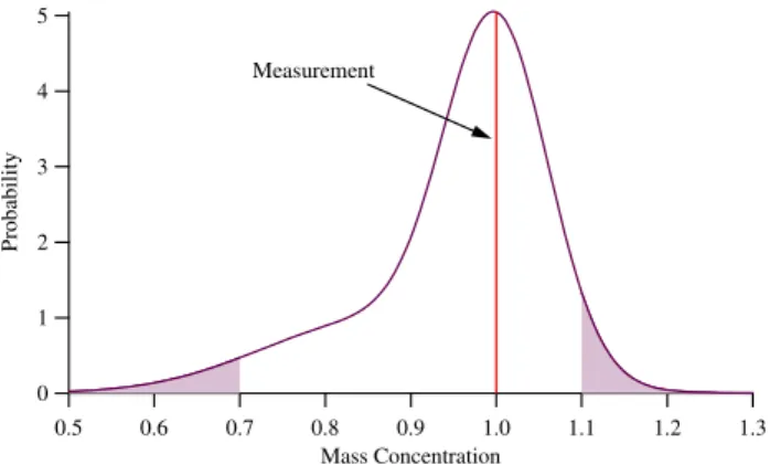
The mass concentrations measured with the Aerodyne AMS during the MCMA-2003 campaign have a range of uncer-tainty of approximately −30% and +10% (Salcedo et al., 2006). This asymmetric likelihood distribution is due to the uncertainty in particle collection efficiency. The mode of the likelihood function will therefore be the observation (i.e., the most likely value is the observation itself), with the probabil-ity densprobabil-ity decreasing from the observation.
5
4
3
2
1
0
Probability
1.3 1.2 1.1 1.0 0.9 0.8 0.7 0.6 0.5
Mass Concentration Measurement
Fig. 3. Asymmetric likelihood function for a hypothetical AMS observation (see Eq. 25) above the detection limit. The observation is 1 (arbitrary units) and has an uncertainty of−30% and +10%. The area of the shaded region is 8%.
p (Xobs|X)=m×N1(µ1, σ1)+(1−m)×N2(µ2, σ2)(24)
where:
m= mixing proportion = 0.7
µ1= the AMS observation =Xobs
σ1=0.061×Xobs
µ2=0.85×Xobs
σ2=0.15*µ2=0.1275×Xobs
Substituting the parameters into the likelihood function yields
p (Xobs|X)=0.7×N (Xobs,0.061Xobs)
+0.3×N (0.85Xobs,0.1275Xobs) (25)
Figure 3 shows the likelihood pdf for an observation of unity (arbitrary units). The most likely concentration is the obser-vation, and the probability that the “true” concentration is greater than 1.1 is 4.3% and less than 0.7 is 3.6% (i.e., there is an 8% chance that the “true” concentration is either below 0.7 or above 1.1).
The AMS observations were measured in 4-min intervals with a 50% duty cycle. The first two minutes of each in-terval were used to characterize the internal particle beam shape and are not included in the averaged data presented here. The detection limits for ammonium, nitrate, and sul-fate were 0.37, 0.05, 0.11µg/m3, respectively. Although the nominal detection limit for chloride is 0.05µg/m3, a higher detection limit was used. The higher detection limit for chlo-ride was selected because on average the chlochlo-ride observa-tions are between one and two orders of magnitude smaller (on a molar basis) than the other inorganic aerosol species, and due to the negative observations reported (see Fig. 12d and Part II). The detection limit used for chloride observa-tions was 0.15µg/m3. Moreover, given the uncertainty of the
55
50
45
40
35
30
25
RH (%)
12:00 AM 4/26/2003
12:00 PM 12:00 AM
4/27/2003
12:00 PM
Date/Time (CDT) 30
25
20
15
T (
o C)
RAMA, hourly averaged RAMA, per minute Averaged temperature (4-min)
RAMA, hourly averaged RAMA, per minute Averaged RH (4-min)
Fig. 4.Temperature and relative humidity profiles from RAMA for La Merced. Where available, we use the per minute data to calcu-late 4-min averages. For periods when the data logger failed, only hourly averaged data was available. For these periods we interpo-lated the hourly averaged data to determine the 4-min averages.
small chloride mass concentrations evidenced by the nega-tive observations, the standard deviation for the chloride like-lihood was doubled for observations between one and two times the detection limit, i.e., for chloride observations be-tween 0.15 and 0.30µg/m3the likelihood function is:
p (Xobs|X)=0.7×N (Xobs,0.122Xobs)
+0.3×N (0.85Xobs,0.255Xobs) (26)
The chloride observations and predictions are discussed fur-ther in Results section and in Part II.
the detection limit, 115 were above 0.30µg/m3and 117 were between 0.15 and 0.30µg/m3.
3.2.4 Likelihood function for temperature and relative hu-midity
Figure 4 shows the observed temperature and relative humid-ity at La Merced. Both the per-minute and per-hour RAMA observations are shown. As can be seen from the gaps in the per-minute data, the data logger failed for extended pe-riods of time. For the pepe-riods where the per-minute data is not available, the hourly averaged data was interpolated. The uncertainty in the averaged temperature and relative humid-ity measurements was assumed to be±0.6◦C and±1.4%, re-spectively, at the 95% confidence level. The likelihood func-tions are:
p (Tobs|T )∼N (Tobs,0.3) (27)
p (RHobs|RH)∼N (RHobs,0.7) (28)
3.3 Selecting the prior
The priorp(θ)represents the uncertainty ofθbefore the data arrives: the prior thus contains all the information available about the unknown variables before the experiment begins. Two desirable characteristics of a prior are that it be well-centered near the actual value of the unknown variables and the uncertainty bands should correspond well to the realized discrepancies between actual and predicted values (Draper, 20063).
Information for the prior may come from previous exper-iments, the scientific literature, expert opinion, constraints provided by knowledge of the physics and chemistry of the system, and so on. For example, if all that is known about a parameter is that it must be greater than zero and below an upper bound, by Laplace’s Principle of Insufficient Reason (Ferson and Ginzburg, 1996) an appropriate prior would be a uniform probability density function:
X∼U[lower bound, upper bound] (29)
In general, some information is almost always available, and one of the advantages of the Bayesian approach is that it pro-vides a formal and intuitive mechanism to utilize this infor-mation.
A natural selection for random variables that must be pos-itive is the lognormal distribution. Kahn provides an elegant explanation for the applicability of the lognormal distribu-tion to air polludistribu-tion concentradistribu-tions (Kahn, 1973). More re-cently, Ott (1990) proposed the theory of successive random dilutions as a physical explanation for the lognormality of pollutant concentrations. The use of lognormal pdf’s to de-scribe pollutant concentrations has been used by a wide vari-ety of researchers (e.g., Beier, 1999; Georgiadis et al., 1998; Hadley and Toumi, 2003; Kan and Chen, 2004; Kao and
Friedlander, 1995; Lorenzini et al., 1994; Lu, 2002; Murphy, 1998; Tripathi, 1994).
The lognormal pdf ofXis given by
p (X)= √ 1
2π σ Xexp −
1 2
ln(X)−µ σ
2!
(30)
Care must be exercised in the notation used: X is the mean of the random variableXwhileµis the mean of the natural logarithm ofX(i.e.,µ=ln(X)).These two size parameters are related by
µ=ln(X)−1
2σ
2
(31) The standard deviation of the natural logarithm ofX is σ. The standard deviation ofX,denoted byσX, is given by
σX= r
e2µ+σ2 eσ2
−1 (32)
Finally, the mode (X)e of the lognormal distribution, which is the most likely value of the distribution, is given by
e
X=eµ−σ2 (33)
Since we are often interested in the most likely value of a variable, ifXis lognormally distributed, this will be denoted as
X∼logN(X, σ )e (34)
3.3.1 Prior for particle phase species
A uniform prior was used for the inorganic AMS species. The maximum concentration observed for ammonium, ni-trate, sulfate, and chloride was 9, 21, 12, and 3µg/m3, re-spectively. None of these maxima is above what one would expect in a polluted atmosphere like Mexico City.
The only inorganic aerosol species for which observations are not available are crustal species. Numerous researchers have highlighted the importance of including crustal species in predicting aerosol behavior (e.g., Ansari and Pandis, 1999a; Jacobson, 1999; Koloutsou-Vakakis and Rood, 1994; Moya et al., 2001). Common crustal elements include Al, Si, Fe, Ca, Mg, K, and Na. Since Al, Si, and Fe are present in the form of stable oxides, they do not participate in reac-tions and do not significantly affect the partitioning of species (Moya et al., 2001). Ca, Mg, K, and Na compounds gener-ally exist as oxides and/or carbonates and can be transformed to water-soluble species, and can affect the distribution of species (Kim and Seinfeld, 1995).
Previous observations have found that geologic material comprises a significant fraction of PM2.5 in Mexico City
25
20
15
10
5
Frequency
50x10-3 40
30 20
10 0
Na (µmol/m3)
80
60
40
20
0
Probability
Observation Frequency Prior Fit for Observations
Prior for Naequiv
Observations ~ logN(12 x 10-3, 0.33)
Naequiv ~ logN(6 x 10⁻³, 0.65)
Fig. 5. Distribution of equivalent sodium concentrations (in µmol/m3)based on PIXE observations (red circles) taken at the CENICA site during MCMA-2003. A lognormal fit (red line) of these observations was fit using the method of moments (Observa-tions∼logN(12×10−3, 0.33)). The lognormal prior for Naequiv
used here (heavy purple line) halved the mode of the fitted dis-tribution and doubled the standard deviation to account for the fact that the PIXE observations provide an upper limit to Naequiv
(Naequiv∼logN(6×10⁻³, 0.65)).
is∼15 km northeast of the site, covers∼12 km2 (Moya et al., 2004) and is a likely source of crustal species. We there-fore need to allow for the presence of crustal material in our calculations.
While crustal material was not measured at La Merced during MCMA-2003, impactor aerosol collection followed by PIXE analysis was conducted at the CENICA site. The experimental setup and results are described in Johnson et al. (2006). Here we use the 6-h averaged concentrations of elemental Na, K, Mg, and Ca from the two smallest stages (0.07–0.34µm and 0.34–1.15µm) to estimate a lognormal prior for equivalent Na, defined as
Naequiv≡Na+K+2Mg+2Ca (35)
where all the concentrations are in molar units (µmol/m3). Moya et al. (2001) found good agreement between the pre-dictions of SCAPE2, which explicitly includes K, Mg, and Ca, with those of ISORROPIA, where crustal species are in-cluded as equivalent Na, when the models were applied to data from the 1997 IMADA-AVER campaign.
The PIXE observations provide an upper limit to the equivalent sodium concentration for two reasons. First, a relatively small critical orifice was selected for the AMS onboard the AML to better sample smaller particles from fresh vehicle exhaust during chase experiments. Thus, the AML AMS size-dependent collection efficiency was shifted to smaller sizes with a 50% cutoff for large particles of
∼0.8µm. On average, approximately half of the
equiva-0.5
0.4
0.3
0.2
0.1
0.0
Probability
0.01 0.1 1 10
NH3 (µmol/m 3
)
20
15
10
5
0
Frequency 6-hour NH
3, La Merced (1997) 100
80
60
40
20
0
Frequency 24-hour NH
3, MCMA (1997)
600
500
400
300
200
100
0
Frequency 6-minute NH
3
, La Merced (2002)
Frequency 6-minuter NH3 (Grutter)
Frequency 6-hour NH3 (IMADA)
Frequency 24-hour NH3 (IMADA)
Prior NH3
NH3 ~ logN(0.5, 0.9)
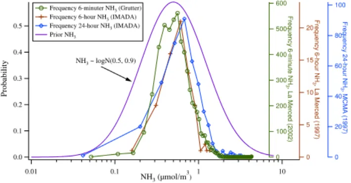
Fig. 6. Distribution of ammonia observations (inµmol/m3)from the 1997 IMADA-AVER campaign and an exploratory campaign held at La Merced during February 2002. The lognormal prior is NH3∼logN(0.5, 0.9).
lent Na is from the smallest stage (0.07–0.34µm) of the im-pactor. Second, the PIXE observations are elemental con-centrations, while we are only interested in the concentration of crustal species that can interact with the other inorganic aerosol species.
Since the PIXE observations provide an upper limit for
Naequivfor our system, we halved the mode and doubled the
standard deviation of the lognormal fit to the PIXE measure-ments found using the method of momeasure-ments (e.g., see p. 1270 in Seinfeld and Pandis, 1998). Figure 5 shows the frequency distribution of the equivalent sodium concentration and the fitted lognormal prior (Observations ∼logN(12×10−3,
0.33), as well as the lognormal prior selected for Naequiv
(Naequiv∼logN(6×10⁻³, 0.65)). Finally, we additionally
im-posed an upper-limit cut-off of Naequiv=80×10−3µmol/m3.
3.3.2 Lognormal prior for NH3and HNO3
The lognormal prior distributions for NH3 and HNO3used
in this work are described in detail by San Martini (2004). Briefly, two sources are used to determine the prior dis-tribution for ammonia: the 1997 IMADA-AVER campaign (Edgerton et al., 1999) and an exploratory campaign under-taken at La Merced during February 2002 (Grutter, 2002). The IMADA-AVER campaign provides 6-h averaged mea-surements at La Merced (only), and 24-h averaged measure-ments at 25 different sites throughout the MCMA (Chow et al., 2002a), while the 2002 exploratory campaign yields 6-min NH3concentrations measured using the same FTIR
sys-tem used here. Figure 6 shows the frequency distribution of the 6-h and 24-h averaged IMADA-AVER observations, the 6-min averaged observations from February 2002, and the fitted lognormal prior (NH3∼logN(0.5, 0.9)).
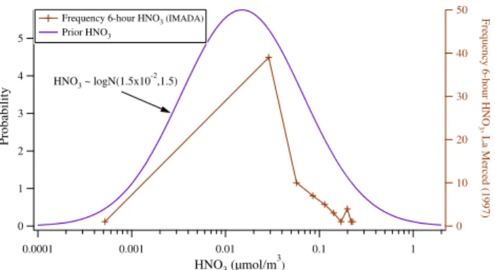
During the IMADA-AVER campaign nitric acid measure-ments were taken as 6-h averages at the La Merced site only. No observations of nitric acid are available from the 2002 exploratory campaign. Given the scarcity of the HNO3
3.3.3 Prior for HCl (g)
To the authors’ knowledge no direct observations of HCl (g) are available for the MCMA. Previous work, however, in-dicates that concentrations of HCl (g) may be appreciable (San Martini et al., 2005). Typical sources of HCl (g) in-clude volatilization of chloride from sea salt particles and other primary particulate matter emissions from natural (e.g., soil dust) and anthropogenic sources. While Mexico City is hundreds of kilometers from the ocean, the dry salt-lake in the northeast of the city is a source of salt particles. Previous work has shown a clear gradient in PM2.5and PM10chloride
concentrations, with decreasing concentrations further from the dry lakebed (San Martini, 2004; San Martini et al., 2005). In addition to the dry lakebed, other sources of (direct or indirect) HCl may be present in the MCMA. The combustion of chlorine- or chloride-containing fossil fuels and the incin-erations of chlorine- or chloride-containing refuse are the two major anthropogenic sources of HCl (Saxena et al., 1993). In the U.S., most of the HCl emissions are believed to be due to (bituminous) coal combustion (Saxena et al., 1993); this will not be the case for Mexico City as there is negligible coal combustion in the MCMA. In general, large anthropogenic sources of molecular chlorine (Cl2)include chemical
pro-duction facilities, water treatment plants, smelters, and paper production operations (Tanaka et al., 2000). Other anthro-pogenic sources that commonly contribute to the chlorine budget include dry cleaning operations and solvent use.
The emissions inventory for chlorine sources in the MCMA is sparse. The 2000 emissions inventory for the MCMA reports usage of chlorine in the production of alu-minum, as well as evaporative emissions of methyl chloro-form and perchloroethylene (Secretar´ıa del Medio Ambiente, 2000). Most emitted organic chloride is expected to be con-verted to HCl given the high level of photochemical activ-ity generally present in the MCMA. Despite the sparseness of the chlorine emissions inventory, the presence of the dry lakebed and the variety of industry in the MCMA suggests appreciable atmospheric emissions of chlorine- and chloride-containing compounds in the MCMA.
In addition to anthropogenic sources, an additional source of chlorine relevant to the MCMA may be the volcano Popocat´epetl located southeast of the MCMA. Volcanoes are a major source of HCl to the atmosphere. Allen et al. (2002) measured emissions from the Masaya Volcano, Nicaragua, and observed concentrations of HCl up to 1300µg/m3. Given the predominant winds, the relatively low volcanic activity, and the distance of the volcano from the city (ap-proximately∼60 km from the center of Mexico City), it is unlikely that emissions from the volcano will significantly impact concentrations in the MCMA. However, there may be episodes of higher than normal volcanic activity that co-incide with winds from the southeast that contradict this as-sumption. Raga et al. (1999) found that aerosol composition in Mexico City is affected by emissions from Popocat´epetl.
5
4
3
2
1
0
Probability
0.0001 0.001 0.01 0.1 1
HNO3 (µmol/m
3 )
50
40
30
20
10
0
Frequency 6-hour HNO
3, La Merced (1997)
Frequency 6-hour HNO3 (IMADA)
Prior HNO3
HNO3 ~ logN(1.5x10
-2
,1.5)
Fig. 7. Distribution of nitric acid observations (in µmol/m3) from the 1997 IMADA-AVER campaign. The lognormal prior is HNO3∼logN(1.5×10⁻², 1.5).
They suggest that recirculating flows as observed by Fast and Zhong (1998) would provide the mechanism to trans-port pollutants from aloft into the city. In addition, Moya et al. (2003) examined size-differentiated aerosol particles dur-ing December 2000–October 2001 and found significantly higher sulfate concentrations during April and June. The authors attribute this observation to an increase in volcanic activity and predominantly easterly winds (i.e., from the vol-cano to the city) during this period, as well as ambient con-ditions that favor sulfate production (high humidity). Thus, given appropriate meteorological conditions and volcanic ac-tivity, Popocat´epetl may contribute to HCl concentrations in the MCMA.
Finally, a characteristic of the air pollution in the MCMA that is of particular relevance in the question of HCl con-centrations is the high concon-centrations of alkanes (Blake and Rowland, 1995). Chlorine radicals react rapidly with alka-nes via hydrogen abstraction to form HCl (g). Therefore, an urban atmosphere with high concentrations of alkanes and a source of chlorine radicals is likely to have appreciable con-centrations of HCl (g).
With no measurements of HCl (g) available for the MCMA, we turn to observations of HCl in other locations to estimate the likely range of HCl (g) concentrations. San Mar-tini (2004) reviewed ambient HCl concentrations in urban lo-cations worldwide, including lolo-cations close and far from the coast. Figure 8 summarizes this review, where for each litera-ture source the minimum and maximum observed concentra-tion are shown; the units of the ordinate are arbitrary. Also shown is the assumed prior (HCl∼logN(0.02, 1.4)), which allows for HCl concentrations an order of magnitude greater and smaller than the largest and smallest observation. 3.4 Selecting the probing distribution
5
4
3
2
1
0
Probability
0.0001 0.001 0.01 0.1 1 10
HCl (µmol/m3)
Prior HCl Saxena et al., 1993 Sturges and Harrison, 1989 Sturges and Harrison, 1989 Matusca et al., 1984 Harrison and Allen, 1990 Harrison and Allen, 1990 DaRoche et al., 2003 Cofer et al., 1985 Grossjean, 1990 Solomon et al., 1988 Solomon et al., 1988 Okita and Ohta, 1979 Farmer and Dawson, 1982 Walker et al., 2004 Matsumot and Okita, 1998 Zimmerling et al., 1996
Fig. 8. Observed urban HCl concentrations (in µmol/m3) in the literature and the proposed lognormal prior distribution, HCl∼logN(0.02, 1.4). The units of the literature data for the ordi-nate are arbitrary. For each literature source the minimum and max-imum reported concentration are shown. The Sturges and Harrison (1989) data are 7-day and 24-h samples; the Harrison and Allen (1990) data are 24-h and 3-h samples; the Solomon et al. (1988) data are annual and 24-h maximum samples. San Martini (2004) provides a review of the literature sources.
Markov steps. The question of what is the “best” probing dis-tribution for a particular problem is a question that has bedev-iled MCMC practitioners from the inception of the method to this day. In part, this is because essentially any probing distri-bution will (eventually) work: the stationary distridistri-bution for just about any probing distribution is the desiredp(θ|Data) (Gilks et al., 1996). To date, no one has established a general method of choosing a probing distribution that always leads to a well-mixed chain. Given this caveat, two suggested char-acteristics of a successful probing distribution are (Draper, 20063):
1. Choose a probing distribution that approximates an overdispersed (i.e., with a larger variance) version of the posterior distribution that is being sampled from Gel-man and Rubin (1992);
2. Choose a probing distribution whose expected value for each proposed move is to stay put, i.e., E(θ∗|θt)=θt, whereθ∗andθt, are the proposed and current states. A symmetric probing distribution, as originally suggested by Metropolis et al. (1953), fulfills the second characteristic. A symmetric probing distribution (i.e.,PD(θ∗|θ)=PD(θ |θ∗))
facilitates the exploration of the entire solution space by as-signing equal probability to left and right moves from the current position.
θis a ten-dimensional vector comprising 9 continuous (T, RH, NH3, HNO3, HCl, NH4, Na, NO4, SO4, Cl, H2O) and
one binary(M)variable. The initial guess used to determine the first Markov step are the observations themselves, where the FTIR rather than the TILDAS and NOzobservations were
used for the ammonia and nitric acid concentrations. The
60
40
20
NH
3
(ppbv)
12:00 AM 4/26/2003
12:00 PM 12:00 AM 4/27/2003
12:00 PM
Date/Time (CDT) 60
50
40
30
20
10
0
NH
3
(ppbv)
(a)
(b)
FTIR (4-min) TILDAS (4-min) Mode 95% CI
0.6 0.4 0.2 0.0
Probability
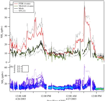
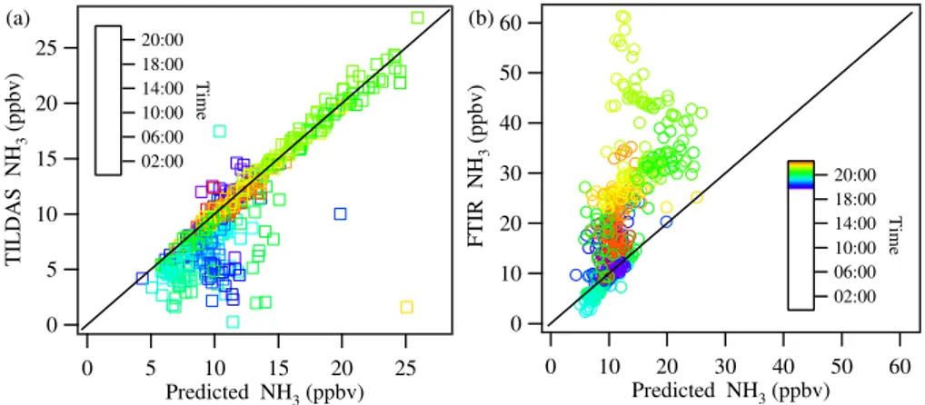
Fig. 9. (a)4-min averaged ammonia observations at La Merced between 25 April and 27 April 2003 taken with the FTIR (red) and TILDAS (green) instruments, and the predicted mode (black) and 95% confidence intervals (dashed black) of the ammonia posterior distribution. (b)Predicted ammonia posterior probability density surface. The model was not run if both ammonia observations were not available; model runs where the Markov Chain did not converge are also not shown (see text).
initial guess for the unobserved concentrations, HCl and Na, were set to 0 ppbv and the concentration required to ensure electroneutrality based on the AMS measurements, respec-tively. The initial guess forMwas zero.
25
20
15
10
5
0
TILDAS NH
3
(ppbv)
25 20 15 10 5 0
Predicted NH3 (ppbv)
02:00 06:00 10:00 14:00 18:00 20:00
Time
60 50
40
30 20
10
0
FTIR NH
3
(ppbv)
60 50 40 30 20 10 0
Predicted NH3 (ppbv)
02:00 06:00 10:00 14:00 18:00 20:00
Time
(a) (b)
Fig. 10.Comparison between the predicted NH3concentration and that observed using the TILDAS(a)and FTIR(b). Only the mode of the
posterior NH3distribution is shown. The points are shaded are shaded by time of day.
M=
MFTIRif 0≤u≤0.5
MTILDASif 0.5< u≤1.0 (36)
A well-chosen probing distribution will favor convergence. We want a Markov chain that mixes well, or, in the words of Draper, “that moves around freely, happily jumping all over the place” (Draper, 20063). A MCMC simulation with either too high or low an acceptance probability is sus-picious: a high acceptance probability indicates that the Markov steps are too small so that the simulation moves very slowly through the target distribution, while a small accep-tance probability may lead the Markov chain to stand still most of the time. Adaptive Metropolis sampling (Gelman et al., 1996) was used in this work to ensure an optimal accep-tance probability (∼20%).
In sum, the MCMC method was applied independently to each set of observations, which comprise temperature, rela-tive humidity, both ammonia observations, nitric acid, and the particle concentrations of ammonium, nitrate, sulfate, and chloride. Each set of observations is a 4-min average, and a total of 612 sets of observations were analyzed.
4 Results
Figure 9a shows the observed and predicted ammonia con-centrations for the period of study. Shown are both the long-path and point observations, as well the mode (black) and 95% confidence interval (dashed black) of the NH3
poste-rior distribution. The NH3posterior probability density
sur-face is shown in Fig. 9b. The model is able to reproduce the observations well when the two ammonia time series agree. The most significant discrepancies between the two ammo-nia time series are evident at night and in the morning hours; during these times, the NH3posterior probability density is
centered on the TILDAS observations. This means that dur-ing these periods, given our understanddur-ing of aerosol
ther-modynamics, the TILDAS observations are more consistent with the temperature, relative humidity, AMS, and gas-phase observations. As will be discussed later, the open-path instru-ment apparently detected a source of ammonia that was not seen in the point measurement. Note that the predicted 95% confidence interval encompasses the long-path FTIR obser-vations, indicating that the FTIR observations are plausible, and that the Markov Chain has explored the entire solution space.
During the afternoon of 26 April 2003, the NH3
poste-rior probability density is more closely centered on the FTIR than TILDAS observations. In this period the FTIR observa-tions are∼3 ppbv larger than the TILDAS observations; this discrepancy is within the uncertainty of the two time series. Figures 10a and b compare the mode of the NH3posterior
distribution with the FTIR and TILDAS observations, where the points are colored by the time of day.
Figure 11 shows the observed and predicted nitric acid concentrations. The observed nitric acid concentrations are low (∼5 ppbv) at night and in the early morning. At approx-imately 11:00 a.m. the concentrations of nitric acid start to increase: this increase occurs despite the rise in the bound-ary layer, clearly pointing to photochemical production of HNO3from rush-hour NOxemissions. The maximum nitric
acid concentration is at∼03:00 p.m. The model captures this diurnal profile well on 26 April 2003. On 27 April 2003 the model appears to over-predict afternoon nitric acid concen-trations. Moreover, nitric acid concentrations at night and during the morning (before∼11:00 a.m.) are predicted to be significantly below the observations. It is during these peri-ods when the concentrations of HNO3are lowest and closest
or below the minimum detection limit.
40
30
20
10
0
HNO
3
(ppbv)
12:00 AM 4/26/2003
12:00 PM 12:00 AM 4/27/2003
12:00 PM
Date/Time (CDT)
40
30
20
10
0
-10
NO
z (ppbv)
40
30
20
10
0
HNO
3
(ppbv)
(a)
(b)
FTIR (4-min) NOz (4-min)
Mode 95% CI
4 2 0
Probability
Fig. 11. (a)4-min averaged nitric acid (red) and NOz(green)
ob-servations at La Merced between 25 April and 27 April 2003, and mode (black) and 95% confidence intervals (dashed black) of the nitric acid posterior distribution.(b)Predicted nitric acid posterior probability density surface.
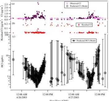
the model has no such difficulties here. The chloride concen-trations deserve particular mention. The top panel of Fig. 14 shows the chloride observations, where only those observa-tions above the detection limit (0.15µg/m3)are shown, as well as the mode of the predicted chloride posterior dis-tribution (black squares). The model accurately predicts the chloride observations when the chloride observations are consistently above the detection limit (∼01:00 a.m. to
∼11:00 a.m.). The HCl (g) concentrations are well con-strained in this period, with concentrations generally on the order of ppbv, though higher concentrations are predicted on the 27th (on the order of 10 ppbv). In particular, the concentration of HCl (g) is predicted to go from sub-ppbv in the early morning hours to ∼1 ppbv at 09:30 a.m. (see Fig. 14c). The concentration of HCl (g) is predicted to in-crease to ∼5 ppbv until ∼10:30 a.m., at which point the predicted aerosol chloride continues to match the observa-tions well. After this the HCl (g) concentraobserva-tions increase to
∼10 ppbv and higher; however, despite these high gas-phase concentrations, the chloride is predicted to partition mostly to the gas-phase, and the aerosol chloride predictions and ob-servations no longer match well. This behavior is also seen in the afternoon periods, where occasionally the AMS chloride observation is above the detection limit. During these peri-ods the Markov Chain will search in extremely high HCl (g) concentration solution space (∼100 ppbv), and still the most likely aerosol phase chloride concentration is negligible. The FTIR setup has not been optimized for detection of HCl (g);
8
6
4
2
NH
4
(µg/m
3 )
12:00 AM 4/26/2003
12:00 PM 12:00 AM
4/27/2003
12:00 PM
Date/Time (CDT) 25
20
15
10
5
0
NO
3
(µg/m
3 )
10 8 6
4 2
SO
4
(µg/m
3 )
3.0
2.0
1.0
0.0
Cl (µg/m
3 )
Detection Limit
AMS NH4
AMS NO3
AMS SO4
AMS Cl
Mode 95% CI
Fig. 12.Predicted (black) and observed (colored) concentrations of ammonium, nitrate, sulfate and chloride at La Merced. The black dashed lines are the predicted 95% confidence intervals; the mea-surement uncertainty is +10%,−30%. The model was not run if both ammonia observations were not available; model runs where the Markov Chain did not converge are not shown (see text).
however, it is expected that it would detect concentrations above 5 ppbv, and certainly concentrations of∼100 ppbv. No such signal was detected.
In sum, when the aerosol chloride concentration is con-sistently above the 0.15µg/m3detection limit, the model is able to accurately reproduce the aerosol chloride concentra-tions. During these periods predicted HCl (g) concentrations are well constrained and on the order of a couple ppbv. Con-versely, when the aerosol chloride signal only occasionally goes above the detection limit, the model either fails to match the aerosol phase concentrations or predicts gas phase con-centrations that are unreasonably high.
4.1 Deliquescence versus efflorescence
12 10 8 6 4 2 0
Predicted SO
4
(µg/m
3 )
12 10 8 6 4 2 0
Observed SO4 (µg/m3)
20
15
10
5
0
Predicted NO
3
(µg/m
3 )
20 15 10 5 0
Observed NO3 (µg/m3) 10
8
6
4
2
0
Predicted NH
4
(µg/m
3 )
10 8 6 4 2 0
Observed NH4 (µg/m3)
3.0 2.5 2.0 1.5 1.0 0.5 0.0
Predicted Cl (µg/m
3 )
3.0 2.0
1.0 0.0
Observed Cl (µg/m3)
Detection Limit
(a) (b)
(c) (d)
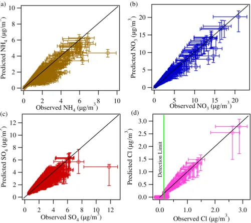
Fig. 13. Correlation plots for(a)ammonium,(b)nitrate,(c)sulphate, and(d)chloride for La Merced. The error bars for the predictions represent the 95% confidence interval; the measurement uncertainty is +10%,−30%. The detection limit for chloride is 0.15µg/m3.
metastable behavior (San Martini, 2004). We therefore inves-tigated the effect of assuming the aerosols were metastable (wet) for the period (04:42 a.m.–11:22 a.m.) on 26 April 2003. During this period the RH started at 49%, reached a maximum of 56%, and then decreased to 34%. The chlo-ride concentration was consistently above the detection limit between 04:42 a.m. and 10:06 a.m. Subsequent to this, the chloride signal varied between being above and below the detection limit until∼11:00 a.m., after which the signal re-mained below the detection limit. We examined the effect of assuming the aerosols were in the metastable branch for this period only because the activity coefficient model used by ISORROPIA breaks down at high ionic strengths.
Differences between the predicted aerosol phase concen-trations for the stable versus metastable case were found to be negligible (see Fig. 15). Similarly, the predicted ammo-nia concentrations for the two cases are very similar (see Fig. 16). Conversely, differences between the predicted gas phase nitric and hydrochloric acid are evident (see Figs. 17 and 18), where in both cases the acid concentrations are slightly higher for the metastable case. The available data are insufficient to discriminate between stable and metastable behavior in this case given the excellent agreement between the ammonia and aerosol phase predictions for the two cases, as well as the uncertainties in the nitric acid observations.
Finally, it is interesting to note that despite the high con-centrations of ammonia observed at La Merced, when the aerosols are assumed to be metastable they are predicted to be acidic. The mode of the pH posterior distribution varies between 2.5 and 4.0 pH units during this period. Note, how-ever, that after∼10:00 a.m. the ionic strength of the aerosols is predicted to be higher than 60 mol/kg. The errors associ-ated with the activity coefficient model used by ISORROPIA are significant at these high ionic strengths. Excluding these points yields an average ionic strength of 41 mol/kg. 4.2 Equilibrium constant KP(NH4NO3)
As discussed in Sect. 3.1, the value of the equilibrium con-stant used by ISORROPIA for the dissociation of solid ammonium nitrate was changed based on the work of Mozurkewich (1993). Figures 19 and 20 compare the ob-servations with the model predictions of NH3 and HNO3,
and Fig. 21 compares the mode of the NH3, HNO3, and
HCl distribution, respectively, predicted using the origi-nal Kp(NH4NO3) based on the thermodynamic tables of
Wagman et al. (1982) and the modified Kp(NH4NO3) of
Mozurkewich (1993). Differences between the NH3 and
HCl concentration for the two cases are small; for HNO3
4 6 8
1
2 4 6 8
10
2 4 6 8
100
HCl (ppbv)
12:00 AM 4/26/2003
12:00 PM 12:00 AM 4/27/2003
12:00 PM
Date/Time (CDT) 2.5
2.0 1.5 1.0 0.5 0.0
Cl (µg/m
3)
0.2 0.1 0.0
Residual Cl (µg/m
3)
(a)
(b)
(c)
Predicted HCl (Mode) Observed Cl Predicted Cl (Mode)
Residual Cl
Fig. 14. (a)Predicted (mode) and observed aerosol chloride con-centrations above the detection limit,(b)residual (observed – pre-dicted) aerosol chloride concentrations.(c)Posterior distribution of HCl (g) concentrations, where the points represent the mode of the probability density function and the error bars are the 95% confi-dence intervals.
formulation of ISORROPIA results in HNO3concentrations
that are∼20% higher. At night and during the early morning hours the model predictions of HNO3are below the
observa-tions regardless of which equilibrium constant is used. The over-prediction of HNO3 for the afternoon of the 27th
dis-cussed previously is exacerbated by the use ofKp(NH4NO3)
based on Wagman’s data (see Fig. 20). We wish to em-phasize, however, that carefully controlled laboratory rather than field conditions are a more appropriate means to deter-mine and validate thermodynamic parameters. Regardless of which value ofKp(NH4NO3)is used, the NH3TILDAS
point observations are more consistent with all the available measurements and our knowledge of thermodynamics.
5 Conclusions
ISORROPIA was embedded in a Markov Chain Monte Carlo algorithm to produce a powerful tool to analyze concentra-tions of inorganic aerosol and gas-phase precursors. The method allows for the direct incorporation of measurement uncertainty, provides a formal framework for including prior knowledge and datasets of different quality. The method was successfully applied to data taken at La Merced during the MCMA-2003 field campaign. The model was able to repro-duce observed aerosol concentrations extremely well, as well as provide an excellent constraint for gas-phase concentra-tions.
2.0
1.0
0.0
Cl (µg/m
3 )
6:00 AM 4/26/2003
8:00 AM 10:00 AM
Date/Time (CDT) 6
5 4 3 2 1
SO
4
(µg/m
3 )
20
15
10
5
0
NO
3
(µg/m
3 )
8
6
4
2
0
NH
4
(µg/m
3 )
Stable Metastable
AMS NH4
AMS NO3
AMS SO4
AMS Cl
Fig. 15. Observed and predicted aerosol ammonium, nitrate, sul-fate, and chloride concentrations. The predicted concentrations are assuming the aerosols are in the deliquescence (black) and efflores-cence (light blue) branch. Only the mode of the aerosol posterior probability function is shown.
5 6 7 8 9
10
2 3 4 5
NH
3
(ppbv)
6:00 AM 4/26/2003
8:00 AM 10:00 AM
Date/Time (CDT)
Stable (Mode) Stable 95% CI Metastable (Mode) Metastable 95% CI
Fig. 16. Predicted ammonia concentrations for the stable (black) and metastable (light blue) case. The solid lines are the mode of the distribution and the dashed lines represent the 95% confidence interval.