www.geosci-model-dev.net/3/391/2010/ doi:10.5194/gmd-3-391-2010
© Author(s) 2010. CC Attribution 3.0 License.
Geoscientific
Model Development
Description and evaluation of GMXe: a new aerosol submodel
for global simulations (v1)
K. J. Pringle1,2, H. Tost1, S. Message1, B. Steil1, D. Giannadaki1, A. Nenes3, C. Fountoukis4, P. Stier5, E. Vignati6, and J. Lelieveld1,7
1Max Planck Institute for Chemistry, Mainz, Germany
2School of Earth and Environment, University of Leeds, Leeds, UK
3Schools of Earth & Atmospheric Sciences and Chemical & Biomolecular Engineering, Georgia Institute of Technology,
Atlanta, GA, USA
4Institute of Chemical Engineering and High Temperature Chemical Processes, Foundation for Research and Technology –
Hellas, Patras, Greece
5Atmospheric, Oceanic and Planetary Physics, Department of Physics, University of Oxford, Oxford, UK 6Joint Research Centre, Institute for Environment and Sustainability, Climate Change Unit, Ispra, Italy 7The Cyprus Institute, Energy, Environment and Water Research Centre, Nicosia, Cyprus
Received: 19 April 2010 – Published in Geosci. Model Dev. Discuss.: 20 May 2010 Revised: 30 August 2010 – Accepted: 2 September 2010 – Published: 10 September 2010
Abstract. We present a new aerosol microphysics and gas aerosol partitioning submodel (Global Modal-aerosol eXten-sion, GMXe) implemented within the ECHAM/MESSy At-mospheric Chemistry model (EMAC, version 1.8). The sub-model is computationally efficient and is suitable for medium to long term simulations with global and regional models. The aerosol size distribution is treated using 7 log-normal modes and has the same microphysical core as the M7 sub-model (Vignati et al., 2004).
The main developments in this work are: (i) the extension of the aerosol emission routines and the M7 microphysics, so that an increased (and variable) number of aerosol species can be treated (new species include sodium and chloride, and potentially magnesium, calcium, and potassium), (ii) the coupling of the aerosol microphysics to a choice of treat-ments of gas/aerosol partitioning to allow the treatment of semi-volatile aerosol, and, (iii) the implementation and eval-uation of the developed submodel within the EMAC model of atmospheric chemistry.
Simulated concentrations of black carbon, particulate or-ganic matter, dust, sea spray, sulfate and ammonium aerosol are shown to be in good agreement with observations (for all species at least 40% of modeled values are within a factor of 2 of the observations). The distribution of nitrate aerosol is compared to observations in both clean and polluted regions.
Correspondence to: K. J. Pringle
Concentrations in polluted continental regions are simulated quite well, but there is a general tendency to overestimate nitrate, particularly in coastal regions (geometric mean of modelled values/geometric mean of observed data≈2). In all regions considered more than 40% of nitrate concentra-tions are within a factor of two of the observaconcentra-tions. Marine nitrate concentrations are well captured with 96% of mode-led values within a factor of 2 of the observations.
1 Introduction
The importance of aerosol for climate and atmospheric pro-cesses has driven the development of global aerosol models with a wide range of complexities. The majority of these schemes treat 5 key aerosol species: black carbon, particu-late organic carbon, sulfate, mineral dust and sea spray (for a review see Textor et al., 2006). Aerosol nitrate has received less attention despite it being a potentially important contri-butor to aerosol burden, particularly in highly industrialised regions (e.g. Malm et al., 2004; Zhang et al., 2007).
aerosol) and is a function of temperature, pressure and the aerosol chemical composition. A number of global aerosol models that can treat nitrate aerosol exist, and studies pre-dict nitrate to be an important aerosol component under both present day (e.g., Adams et al., 1999, 2001; Metzger et al., 2002; Bauer and Koch, 2005; Myhre et al., 2006; Feng and Penner, 2007) and future conditions (e.g. Derwent et al., 2003; Bauer et al., 2007; Pye et al., 2009). The Fourth As-sessment Report from the Intergovernmental Panel on
Cli-mate Change (Forster et al., 2007) estiCli-mated the radiative
forcing of nitrate aerosols to be−0.1±0.1 W m−2, but noted that the number of model studies which have calculated this parameter is “insufficient for accurate characterisation of the magnitude and uncertainty of the radiative forcing”. There is therefore a continued need to develop aerosol models that can treat nitrate aerosol and can be used for climate and radi-ation studies.
Including the partitioning of nitrate between the gas and aerosol phases in models has an additional benefit in that it also allows the more detailed treatment of ammonium aerosol. Models that do not consider the partitioning typ-ically assume that all sulfate is in the form of ammonium sulfate, thus the concentration of ammonium in the aerosol is simply implied from the concentration of sulfate. Treat-ment of the partition of the sulfate/nitrate/ammonium system allows the on-line calculation of ammonium concentrations, rather than assuming a fixed sulfate to ammonium ratio.
The purpose of the present paper is to introduce and doc-ument a new aerosol microphysics submodel called GMXe. The model is based on the M7 aerosol microphysics model (Wilson et al., 2000; Vignati et al., 2004; Stier et al., 2005) but it has a number of new features which make it a useful development for air quality and climate modelling studies. Firstly, GMXe can treat a wider range of species than tra-ditional aerosol models; in addition to the standard species (black carbon, particulate organic matter, dust and sea spray), GMXe can also treat sodium, chloride, magnesium, potas-sium and calcium. The model also includes treatment of semi-volatile inorganic partitioning (e.g., nitrate and chlo-ride). The model is introduced in Sects. 2 and 3 and com-pared against observations in Sect. 4.
2 Host model description
2.1 The ECHAM/MESSy Atmospheric Chemistry (EMAC) model
The Global Modal-aerosol eXtension (GMXe) submodel is implemented within the ECHAM/MESSy Atmospheric Chemistry model (EMAC, Version 1.8) – a combination of the ECHAM5 general circulation model (Roeckner et al., 2006, version 5.3.0.1) and the Modular Earth Submodel Sys-tem (J¨ockel et al., 2005, 2006). For a full description of the EMAC model and evaluation see J¨ockel et al. (2005, 2006)
or http://www.messy-interface.org. The MESSy system is modular and all submodels (including GMXe) follow strict coding standards to allow portability and modularity.
Various resolutions are possible in EMAC; in this study a spectral resolution of T42 degrees and 19 vertical levels was used. The model was “nudged” towards actual meteorology using ECWMF reanalysis data. In the simulations used in this work, the model was run for two years (2001 and 2002) with a spin-up period of six months.
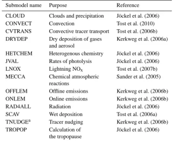
A summary of the EMAC sub-modules used in this study is presented in Table 1. Gas-phase chemistry is simulated in EMAC with the MECCA submodel (Sander et al., 2005, Sect. 2.2). The wet deposition of gases and aerosols (initi-ated by both nucleation and impaction scavenging) is tre(initi-ated within the SCAV submodel (Tost et al., 2006b, 2007a), which describes scavenging due to convective and large-scale rain, snow and ice. Dry deposition is treated using the big leaf approach within the DRYDEP submodel (Ganzeveld and Lelieveld, 1995; Kerkweg et al., 2006a). Sedimentation of all aerosol types is treated within the SEDI submodel (Kerk-weg et al., 2006a). Emission of gas and aerosols is treated by the ONLEM and OFFLEM routines (Kerkweg et al., 2006a). The other submodels used in this study are CONVECT (Tost et al., 2006b), LNOX (Tost et al., 2007b), TNUDGE (Kerk-weg et al., 2006b), as well as CLOUD, CVTRANS, JVAL, RAD4ALL, and TROPOP (J¨ockel et al., 2006).
2.2 Gas phase chemistry
The EMAC model calculates fields of gas phase species on-line through the MECCA submodel (via the Module Effi-ciently Calculating the Chemistry of the Atmosphere Sander et al., 2005). MECCA calculates the concentration of a range of gas phase species, including aerosol precursor species such as SO2, NH3, HNO3, DMS, H2SO4and DMSO. The
concentrations of the major oxidant species (OH, H2O2,
NO2, and O3) are also calculated online (see Sander et al.,
2005; J¨ockel et al., 2006).
In GMXe the loss of gas phase species to the aerosol through heterogeneous reactions (e.g., N2O5to form HNO3)
is treated using the HETCHEM submodel (e.g. J¨ockel et al., 2006).
2.3 Aqueous phase chemistry
The aqueous phase oxidation of SO2and the uptake of HNO3
and NH3in cloud droplets is an important source of aerosol
growth, the particles can be re-partitioned into other modes within GMXe (using the mode merging algorithm of Vignati et al., 2004).
2.4 Wet scavenging of aerosol
Wet removal of aerosol particles occurs via both nucleation and impaction scavenging. Whereas impaction scavenging is caused by the physical process of falling droplets and crystals and affects both hydrophobic and hydrophilic particles, nu-cleation scavenging (removal of activated aerosol particles) is only calculated for the hydrophilic modes. To determine the scavenged fraction of the particles per mode an empirical formula (see Tost et al., 2006a) is applied.
The material incorporated in cloud droplets via nucleation scavenging can either be (i) removed from the atmosphere based on the precipitation formation rate or (ii) released back into the aerosol phase after cloud evaporation. Furthermore, it can participate in chemical reactions in the aqueous phase (see above).
Due to the assumed internal mixing of the particles within the hydrophilic modes when hydrophillic aerosol are scav-enged any coated hydrophobic cores, e.g. OC, BC are also scavenged. At present, the information of the nucleation scavenged particles is not used for determining the cloud droplet number concentration, which is in the current sim-ulations a climatological value only.
2.5 Bulk emissions
Throughout this manuscript we make the distinction between aerosol species where the chemical composition is resolved and the individual ions that make up the compound are known (e.g. sodium or chloride) and species where the chem-ical composition is unresolved (here termed “bulk” species). Bulk species are generic aerosol species such as “dust” or “black carbon” which (in the atmosphere) are known to con-tain a range of different species, but which are treated as chemically inert within the model. With bulk species there is no resolution of the individual species that comprise the aerosol type.
In the model setup used in this study all primary (bulk) aerosol emissions are taken from the AEROCOM (an AEROsol module inter-COMparison in global models, http:// nansen.ipsl.jussieu.fr/AEROCOM/) recommendations com-piled by Dentener et al. (2006). These emissions are all re-presentative of the year 2000. The division of bulk emission streams to speciated emissions is treated within GMXe, and is described in Sect. 3.5.
2.5.1 Dust and sea spray
The mass flux of sea spray and mineral dust are treated us-ing monthly mean emission files (Dentener et al., 2006), thus emissions are “offline” and not dependent on the sim-ulated meteorology. Offline emission fields are used in this
Table 1. Summary of the EMAC submodels used in this study.
HETCHEM is used to calculate stratospheric reaction rates (and the rate of conversion of N205in the troposphere). TNUDGE nudges
concentrations of long lived species (e.g. CH4and N2O) at the
sur-face.
Submodel name Purpose Reference
CLOUD Clouds and precipitation J¨ockel et al. (2006)
CONVECT Convection Tost et al. (2010)
CVTRANS Convective tracer transport Tost et al. (2006b) DRYDEP Dry deposition of gases Kerkweg et al. (2006a)
and aerosol
HETCHEM Heterogenous chemistry J¨ockel et al. (2006) JVAL Rates of photolysis J¨ockel et al. (2006) LNOX Lightning NOx Tost et al. (2007b) MECCA Chemical atmospheric Sander et al. (2005)
reactions
OFFLEM Offline emissions Kerkweg et al. (2006b) ONLEM Online emissions Kerkweg et al. (2006b) RAD4ALL Radiation J¨ockel et al. (2006) SCAV Wet deposition Tost et al. (2006a) TNUDGEa Tracer nudging Kerkweg et al. (2006b) TROPOP Calculation of J¨ockel et al. (2006)
the tropopause
study given their extensive use and evaluation in a number of aerosol model frameworks (e.g. Textor et al., 2007). In tak-ing this approach we acknowledge that the model will likely underestimate the inter-seasonal variability of dust and sea spray aerosol.
For sea spray we convert the mass flux to a number flux assuming a radius on emission of 0.156 and 0.85 µm for the accumulation and coarse modes, respectively. This flux was calculated for AEROCOM using the sea spray flux parametrisation of Gong (2003). Mineral dust fields were calculated using the parametrisation of Ginoux et al. (2001) as used by Ginoux et al. (2003). We split the total dust mass flux between the coarse (98.6%) and the accumulation (1.4%) modes and emit with a number mean radius of 0.21 and 0.65 µm, respectively (Dentener et al., 2006). EMAC also has the option to calculate the emission of sea spray and mineral dust aerosol on-line (Kerkweg et al., 2006b), but in the simulations presented in this work this option was not used.
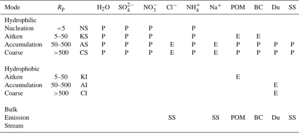
Table 2. Example setup of the GMXe submodel, as used in this work (other combinations/setups are possible). Aerosol species are distributed
between the 4 hydrophilic and 3 hydrophobic aerosol modes. E = Emitted into the mode, P = Permitted in the mode. BC = black carbon, POM = particulate organic matter, SS = sea spray, Du = dust.Rp=radius (nm).
Mode Rp H2O SO24− NO3− Cl− NH+4 Na+ POM BC Du SS
Hydrophilic
Nucleation <5 NS P P P P
Aitken 5–50 KS P P P P E E
Accumulation 50–500 AS P P P E P E P P P P
Coarse >500 CS P P P E P E P P P P
Hydrophobic
Aitken 5–50 KI E
Accumulation 50–500 AI E
Coarse >500 CI E
Bulk
Emission SS SS POM BC Du SS
Stream
this work we do not treat the partitioning of secondary or-ganic aerosol between the gas and particulate phase; SOA is emitted and transported as a bulk aerosol species (POM).
3 GMXe model description 3.1 Model formulation
The GMXe submodel comprises two parts:
– Microphysics: aerosol microphysics are treated using an extended version of the M7 modal aerosol scheme (Wil-son et al., 2000; Vignati et al., 2004; Stier et al., 2005), which describes the aerosol distribution using 7 inter-acting lognormal aerosol modes; 4 hydrophilic modes and 3 hydrophobic modes. See Table 2 and Sect. 3.2.1.
– Gas/aerosol partitioning: a full thermodynamic treat-ment of gas/aerosol partitioning is prohibitively expen-sive for inclusion in global models, and even simpli-fied thermodynamic models normally require iteration and thus can add significantly to the computational bur-den. In GMXe we have chosen to offer a choice of complexities: partitioning can be treated using either the ISORROPIA-II thermodynamic equilibrium model (Fountoukis and Nenes, 2007), or the EQSAM3 model (Metzger and Lelieveld, 2007).
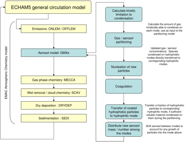
A schematic overview of the GMXe model and how it is im-plemented in EMAC is shown in Fig. 1.
3.2 The aerosol microphysics 3.2.1 The aerosol size distribution
The aerosol size distribution is described by the supposition of 7 interacting lognormal modes (4 hydrophilic and 3 hy-drophobic modes):
n(lnr)= 7 X
i=1 Ni √
2πlnσi
exp −(lnr−lnr¯i)
2
2ln2σi !
(1) where each mode (i) is defined in terms of the number con-centration (Ni), the number mean radius (r¯i) and the
geomet-ric standard deviation (σi).
The aerosol number and mass (the latter of each com-ponent) are calculated prognostically, but following Vignati et al. (2004) and Stier et al. (2005) the geometric standard deviation of the mode is fixed (σ= 2.0 for the coarse hy-drophobic mode, σ= 2.2 for coarse hydrophilic mode and 1.69 for the other modes). The choice ofσ= 2.2 for coarse hydrophilic mode is different to previous implementations of the M7 (Stier et al., 2005; Kerkweg et al., 2007), who use σ= 2.0 (discussed in Sect. 4.2.1).
The 4 hydrophilic modes are arranged to cover the aerosol size spectrum (nucleation to coarse modes) from particles <5 nm radius to those>500 nm (Table 2). Each size range has a fixed size boundary but a variable mean radius. The 3 hydrophobic modes have the same size range, but no hy-drophobic nucleation mode is required (Stier et al., 2005). The aerosol composition within each mode is uniform with size, but the composition can vary between modes.
ECHAM5 general circulation model
Calculate kinetic limitation to condensation
Gas / aerosol partitioning Emissions: ONLEM / OFFLEM
Gas phase chemistry: MECCA
Wet removal / cloud chemistry: SCAV
Dry deposition : DRYDEP
Sedimentation : SEDI Aerosol model: GMXe
E
M
A
C
A
tm
o
s
p
h
e
ri
c
C
h
e
m
is
tr
y
m
o
d
e
l
Nucleation of new particles
Coagulation
Transfer of coated hydrophobic particles
to hydrophilic mode Distribute new aerosol mass / number among
the modes
Calculate the amount of gas kinetically able to condense on each mode, use as input to the
partitioning model
Updated gas / aerosol concentrations. Species condensed on hydrophobic modes directly transferred to
corresponding hydrophilic modes.
Shift aerosol between modes to account for any growth of particles into the mode above Transfer a fraction of hydrophobic
particles to corresponding hydrophilic mode, if sufficient soluble material condensed on
them during the partitioning.
Fig. 1. Graphic summarising the calling sequence of the processes in the GMXe model, implemented within the ECHAM/MESSy
Atmo-spheric Chemistry model.
or type of species – GMXe can treat an increased number of aerosol species compared to the M7 (which simulates 5 aerosol species) and the number of species simulated can be varied to suit the setup required (so ensemble runs of dif-fering complexities can be done).
Table 2 shows the setup of the aerosol model used in this introductory paper. In this work we consider the major ions present within sea spray (sodium and chloride) but neglect more minor marine species (e.g. magnesium) and we also neglect the cations present within mineral dust aerosol or BC (e.g. calcium and potassium). Treatment of these species is also possible in GMXe (Sect. 3.5) but these species will be the focus of future work.
3.2.2 Nucleation of new particles
Nucleation of new particles is calculated as a function of the temperature, relative humidity and the concentration of sulfuric acid (H2SO4). Two binary nucleation schemes are
available in GMXe; the scheme of Vehkamaki et al. (2002) and that of Kulmala et al. (1998). In this work we use the Vehkamaki et al. (2002) scheme, this parametrisation is valid over the range 0.01%<RH<100% and 190 K< T <305.15 K.
3.2.3 Coagulation
Coagulation is treated following Vignati et al. (2004); coagu-lation coefficients are calculated for Brownian motion using Fuchs (1964). In GMXe the coagulation matrix has been generalised to handle a variable number of species per mode. Coagulation can potentially move aerosol from smaller to larger modes and from hydrophobic to hydrophilic modes. As in M7, GMXe assumes that the coagulation of two par-ticles from the same mode will form a new particle in that mode (e.g. KS + KS = KS), and two particles from differ-ent modes will form a new particle in the larger mode (e.g. KS + AS = AS). Coagulation between hydrophilic and hy-drophobic modes produces a new particle in the larger of the hydrophilic modes (e.g. AI + KS = AS) (where KS = Aitken soluble (hydrophilic) and AS = accumulation soluble (hy-drophilic) and AI = Aitken insoluble (hydrophobic)). 3.3 Gas/aerosol partitioning
3.3.1 The ISORROPIA-II model
ISORROPIA-II is an inorganic equilibrium model that is able to calculate the gas/aerosol/solid equilibrium partitioning of the main atmospherically relevant inorganic semi-volatile species (Fountoukis and Nenes, 2007). It is an extension of the ISORROPIA model (Nenes et al., 1998a,b) and is able to treat the interaction of K, Ca, Mg, NH4, Na, SO4, NO3,
Cl, H2O aerosols. Gas-phase species considered are NH3,
HCl, HNO3, H2O; aerosol phase species include all major
ionic and solid salts formed by K, Ca, Mg, NH4, Na, SO4,
NO3, Cl. In cases where aqueous solutions are present, H+,
OH−and undissociated forms of HNO3, NH3, HCl are also considered.
ISORROPIA-II solves for the equilibrium state by con-sidering the chemical potential of the species (Nenes et al., 1998a,b). By considering specific compositional “regimes”, it minimises the number of equations and iterations required. Because of this, it is considered one of the most computation-ally efficient thermodynamic equilibrium models available. In ISORROPIA-II, the aerosol can be in either a thermody-namically stable state (where salts precipitate once the aque-ous phase becomes saturated) or in a metastable state (where the aerosol is composed only of a supersaturated aqueous phase). The model can solve for either: (i) “forward” prob-lems where the total (i.e., gas + aerosol) concentrations are known and the gas/aerosol concentrations are predicted, or (ii) “reverse” problems where the aerosol concentration is known and the gas concentrations are predicted. In this work we use ISORROPIA-II in the “forward” mode.
ISORROPIA-II also offers the options to (i) calculate ac-tivity coefficients on-line or (ii) use pre-calculated look up tables (the latter of which is used in this study). Since its release, ISORROPIA-II has been used in a number of global (Pye et al., 2009) and urban-scale (Fountoukis et al., 2009; Karydis et al., 2010) model studies.
3.3.2 The EQSAM3 model
The EQSAM3 model is a simplified, non-iterative, treatment of gas/aerosol partitioning that uses analytical expressions based on species solubility (Metzger and Lelieveld, 2007). Compared to other treatments of partitioning, EQSAM3 is more flexible as it is easily expandable to treat additional in-organic ions and speciated in-organics. The model can be run in a range of complexities, in this work we consider the same cations as treated by ISORROPIA-II and no speciated organ-ics. Sensitivity to increased complexity will be considered in future work.
EQSAM3 calculates the amount of species partitioning to the aerosol phase through the use of a “neutralisation order”, this order is used to rank the ions in terms of their ability to form a neutral salt. There are two options available to calculate the neutralisation order in EQSAM3:
1. Order calculated online by EQSAM3 (see Metzger and Lelieveld, 2007), based on the deliquescence relative humidity of the species present.
2. Order prescribed according to the Hofmeister series (Hofmeister, 1888; Metzger and Lelieveld, 2007):
(a) Anions: SO42−, HSO4−, NO3−, Cl−, OH−.
(b) Cations: Na+, NH4+, H+.
In this work we use the order prescribed by the Hofmeister series.
The neutralisation order determines which ions are paired to form a salt first; ions are paired by taking the first cation (Na+) and looping over all anions and then then moving to the next cation (NH4+), and so on. In this way neutral
com-pounds are formed using ions at the top of the order first. Pairing is only permitted if there are sufficient cations and an-ions in the solution. Once no more neutral solute can form, any un-paired cations or anions are assumed to stay in the aqueous phase, and un-neutralised gases (NH3, HNO3 and
HCl) are assumed to partition to the gas phase. For semi-volatile species (NH4NO3and NH4Cl), a further loss (from
the aerosol phase) is calculated using a relation based on ac-tivity coefficients (Metzger and Lelieveld, 2007).
EQSAM3 is developed and maintained as part of the ECHAM/MESSy group, and will be further developed to in-clude additional aerosol compounds e.g. sugars.
3.3.3 The aerosol water content
Water is an important parameter as it often constitutes the bulk of the particle volume, and changes in the aerosol wa-ter loading can alwa-ter the aerosol wet radius and thus affect the interaction of the particle with condensable gases and ra-diation. The parametrisation of ambient water uptake varies greatly between aerosol models; ranging from simplified em-pirical parametrisation (e.g. that of Gerber, 1991) to treat-ments that take the activity of multi-component aerosols into account. Textor et al. (2006) found that there was a broad range in aerosol water contents predicted by the AEROCOM models, partly due to the range of parametrisations used. In the setup used in this work, ISORROPIA-II (or EQSAM) is used to calculate water uptake on inorganic species, water uptake onto organic species is not permitted. As the calcula-tion of aerosol water is valid for subsaturated condicalcula-tions only, the relative humidity used within GMXe is set to be<98%. 3.3.4 Non-equilibrium considerations
Meng and Seinfeld, 1996; Wexler and Seinfeld, 1992; Ca-paldo et al., 2000). Non-equilibrium can occur in large parti-cles as they are subject to mass transfer limitations. Assum-ing the whole aerosol size distribution to be in equilibrium will bias the calculation of the amount of aerosol in fine and coarse modes (e.g. Capaldo et al., 2000; Feng and Penner, 2007; Karydis et al., 2010).
Some models account for non-equilibrium conditions by only considering the gas/aerosol partitioning on the fine modes and excluding the formation of sulfate-nitrate-ammonium on coarse mode aerosol (e.g. Pye et al., 2009) or by neglecting the coarse mode aerosol either (i) entirely (e.g. Lauer et al., 2005; Lauer and Hendricks, 2006), or, (ii) par-tially (e.g. Bauer et al., 2007, who neglect nitrate formation on sea salt). But the above approach is at odds with field observations which have shown that a significant amount of nitrate aerosol can be present in the coarse mode (e.g. Pakka-nen, 1996; Zhuang et al., 1999). For example in a field study in two polluted coastal regions Yeatman et al. (2001) found that between 40 to 81% of the total nitrate present in the aerosol phase was found in the coarse mode.
A more sophisticated way of treating the different modes is that of Capaldo et al. (2000) who calculate composition using a hybrid dynamic approach. This hybrid approach has been used in a global aerosol model (Feng and Penner, 2007), but the additional calculation required adds to the computational overhead of the model.
To account for kinetic limitations in GMXe the process of gas/aerosol partitioning is calculated in two stages. In the first stage the amount of gas phase species kinetically
able to condense onto the aerosol (within a timestep) is
cal-culated (assuming diffusion limited condensation, following Fuchs, 1959; Vignati et al., 2004). This calculation of the kinetic limitation to condensation is the same as that used to treat condensation of H2SO4in the M7 (Vignati et al., 2004),
but it has been extended to also treat NH3, HCl and HNO3.
The calculation uses an accommodation coefficient for each species, this was taken as 0.1, 0.064 and 0.09 for HNO3, HCl,
NH3respectively (Vandoren et al., 1990; Hanisch and
Crow-ley, 2003). These values are similar to the values used by Feng and Penner (2007), being 0.193 for HNO3and 0.09 for
NH3.
The second stage of the partitioning is the thermodynamic consideration. Once the total amount of gas that could ki-netically condense to each mode is calculated, the chosen partitioning model (ISORROPIA-II or EQSAM3) is used to re-distribute the mass between the gas and the aerosol phase. Hence, for a low volatility species, e.g. H2SO4, the total
amount that condenses is simply the amount that is kineti-cally able to condense (Vignati et al., 2004; Stier et al., 2005). For a semi-volatile species, only a fraction of the gas that is kinetically able to condense will partition to the aerosol phase (as dictated by the thermodynamics).
3.4 Transfer of aerosol between modes
The aerosol microphysics routines described above can result in aerosol changing from hydrophobic to hydrophilic (e.g. through condensation or coagulation with hydrophilic mate-rial). To account for this in GMXe, the transfer of material from the hydrophobic to the hydrophilic modes is calculated in two places:
1. After coagulation: when a hydrophobic and hydrophilic particle coagulate the resulting mass is assumed to re-side in the hydrophilic mode.
2. After gas/aerosol partitioning: any soluble material that partitions onto the hydrophobic modes is transferred di-rectly to the hydrophilic modes, along with a fraction of the hydrophobic material. The amount of hydropho-bic material transferred (mass and number) is calculated from the fraction of the particles that is able to receive five monolayer coverage of hydrophilic material. The use of a monolayer approach was introduced by Vi-gnati et al. (2004) and used by Stier et al. (2005) to ex-press the ageing of hydrophobic particles into hydrophilic modes. When sufficient hydrophilic material is added to the hydrophobic modes such that “n” monolayers of hydrophilic material could be created, the material is transferred between modes. Vignati et al. (2004) varied “n” in a box model and found that n equal to 1 gave the best agreement to a de-tailed sectional model. In GMXe, n equal to 5 is chosen, as more material is available for condensation compared to Vignati et al. (2004, who treat condensation of H2SO4only).
In GMXe, the larger monolayer threshold gave better com-parison of BC and dust aerosol to observations. The value of n nethertheless is an adjustable parameter in the model (and in other models that take the monolayer approach, for example the GLOMAP-mode model which uses a monolayer threshold of 10; Mann et al., 2010). This larger threshold is in line with the finding of Granat et al. (2010) who exami-ned aerosol concentrations in precipitation in the Maldives and found that soot aerosol could remain hydrophobic for many days after emission. Modal aerosol models (including GMXe) would benefit from additional laboratory and field studies into particle ageing which could better constrain how much hydrophilic material is required to make a hydrophobic particle hydrophilic.
will then be re-distributed later). Except for the choice of a larger monolayer threshold, the transfer of the aerosol be-tween modes in GMXe is the same as that of ECHAM HAM (Stier et al., 2005).
3.5 Bulk or speciated emissions
The presence of ions within an aerosol has been shown to affect the balance of gas/aerosol partitioning (e.g. Jacobson, 1999; Metzger et al., 2006; Fountoukis et al., 2009), thus to improve the treatment of semi-volatile species it is impor-tant to consider the chemical makeup of the aerosol and not simply the bulk species. One study that has done this is that of Rodriguez and Dabdub (2004) who sub-divide the emis-sion streams of the bulk dust and sea spray into the ionic constituents (e.g. Na+, Ca2+) in order to simulate the ionic composition for use in calculating the gas/aerosol partition-ing.
GMXe takes a similar approach to that of Rodriguez and Dabdub (2004); it offers the flexibility to subdivide each of the four “bulk” emission streams (BC, POM, SS and Du) into speciated emissions (e.g. Na+, Ca2+, K+). Each “bulk” emission stream (BC, POM, SS or Du) can be either (i) left as bulk or (ii) be semi (or fully) speciated.
For example, the sea spray aerosol can be treated in two different ways:
1. Bulk: the sea spray is emitted into a “bulk” sea spray distribution, which has the same molecular weight and density as NaCl, but the individual ions that comprise the aerosol are not simulated (and therefore not permit-ted to interact with other ions in the calculation of par-titioning).
2. Speciated: the mass flux of emitted sea spray aerosol is split into its constituent ions (Cl−, Na+, SO42−and also
potentially Mg2+, etc.) based e.g. on the ionic compo-sition of sea water. The individual ions are then trans-ported as tracers (and passed into the partitioning rou-tines for thermodynamic calculations).
Similarly the dust, BC and POM emission streams can also be subdivided, e.g. calcium could be emitted as a fixed frac-tion of the dust mass flux. In addifrac-tion to setting up the emis-sion streams, the user can also control which of the simu-lated species is “permitted” to exist in each mode. It is pos-sible to simulate any of the available species in any of the modes (although of course not all combinations are realis-tic). An example model setup is shown in Table 2. The flexible nature of the design allows one to choose the species simulated (and their sources) to suit the problem at hand. The control of the division of bulk emission streams into speci-ated emissions and the switches controlling which species is “permitted” in each mode is controlled via a simple include file. The electronic supplement gives a tutorial to help with the initial model setup.
4 Results and evaluation
The simulations shown in this section were performed with the model setup shown in Table 2. Unless otherwise speci-fied, the calculation of gas/aerosol partitioning was done us-ing the ISORROPIA-II model. Simulated species were BC, POM, bulk sea spray, dust, SO24−, NO−3, NH4+, Na+, Cl−
and H2O. The sea spray flux was divided as follows; 85% by
mass was split to form a flux of Na+and Cl−ions, 5% was assumed to be sodium sulfate and the remaining fraction was assumed to be “bulk” sea salt. This follows the approximate composition of sea water (Castro and Huber, 2003), where the bulk flux comprises species such as marine organics, Mg and K, which are not treated in this setup. The other emis-sions streams were not speciated (bulk only).
4.1 Aerosol number concentration
The aerosol microphysics control the particle number and size distribution. The microphysics used in GMXe are the same as those of the M7 model (as used in a global study by Stier et al., 2005), thus here we only briefly present a sum-mary of the key properties.
As a first evaluation step we present simulated fields of number concentration in the same format as those presented by Stier et al. (2005) using the ECHAM-HAM model. Com-parison of GMXe fields with ECHAM-HAM fields is use-ful as ECHAM-HAM is a well established and widely used aerosol model (e.g. Stier et al., 2006; Lohmann et al., 2007) and the inter-model comparison gives a global overview of the number concentration (per mode) that is not easily achieved from field observations. The zonal mean annual average aerosol number concentrations simulated by GMXe are shown in Figs. 2 and 3. For evaluation, our Figs. 2 and 3 is comparable to the number concentrations shown by Stier et al. (2005) in their Fig. 4.
800 1000 600 400 200 60 80 100
Nucleation Hydrophilic
800 1000 600 400 200 60 80 100
Aitken Hydrophilic
800 1000 600 400 200 60 80 100
Aitken Hydrophobic
Fig. 2. Zonal and annual mean aerosol number concentration
(con-verted to STP conditions at 1013.25 hPa and 273.15 K, cm−3) for the year 2001 for the (top left) nucleation hydrophilic, (bottom left) Aitken hydrophilic and (bottom right) Aitken hydrophobic modes as simulated by GMXe.
at 500 hPa is not simulated in GMXe (number concentrations of 20–50 cm−3are simulated instead), however observations in this region are limited so it is difficult to determine the bias of either model.
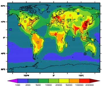
Andreae (2009) collected observed values of condensa-tion nuclei (CN) concentracondensa-tions taken from a range of field campaigns and field sites around the world. The standard definition of the CN concentration is the number of parti-cles with dry diameter>3 nm, but Andreae (2009) also in-cluded some data which used a larger reference diameter. In Fig. 4 we show the annual mean CN concentration simulated by the model, with values summarised by Andreae (2009) over-plotted. Only a qualitative comparison can be made as we compare annual mean model data with observation data taken over a range of time periods (some short term from field campaigns lasting only a few weeks and some multi-annual mean), but to maximise the amount of comparison data we do not exclude short-term data.
The comparison of modelled and observed values shows good agreement; low values (∼200–500 cm−3) are seen in the remote marine regions, and larger values (500– 2000 cm−3) in marine environments influenced by continen-tal outflow. Values larger than 5000 cm−3 are simulated in polluted regions of Europe and Asia, also in line with the observations.
The Global Atmospheric Watch (http://wdca.jrc.it/data/ aerosol program.html) program has collated a range of aerosol data from a number of observation stations. In Fig. 5 we compare simulated aerosol number concentrations
800 1000 600 400 200 60 80 100
Accumulation Hydrophilic
800 1000 600 400 200 60 80 100
Accumulation Hydrophobic
800 1000 600 400 200 60 80 100
Coarse Hydrophilic
800 1000 600 400 200 60 80 100
Coarse Hydrophobic
Fig. 3. As Fig. 2 but for the (top left) accumulation hydrophilic, (top
right) accumulation hydrophobic, (bottom left) coarse hydrophilic and (bottom right) coarse hydrophobic modes.
Fig. 4. Annual mean surface aerosol number concentration (cm−3) compared to observed values (from a range of time periods) col-lected by Andreae (2009). Simulated values show total particle number in the Aitken, accumulation and coarse modes. Observa-tions have a range of cutoff diameters.
Month
CN C
onc
en
tr
a
tion (cm )
-3
104
103
J
F M A M J
J A S O N D
Southern Great Plains (36N, 97W)
Month
CN C
onc
en
tr
a
tion (cm )
-3
103 104
J
F M A M J
J A S O N D
Bondville (40N, 88W)
Month
CN C
onc
en
tr
a
tion (cm )
-3
10
10
10
101 2 3 4
J F M A M J
J A S O N D
Point Barrow (71N, 156W)
Month
CN C
onc
en
tr
a
tion (cm )
-3
10
10
10
101 2 3 4
J
F M A M J
J A S O N D
Pallace (68N, 24E)
Fig. 5. Seasonal cycle of aerosol number concentration (cm−3) in four locations as measured by the Global Atmopsheric Watch net-work. Lines show modelled values for 2001 (black) and 2002 (blue) and observed values for 2001 (red dash) and 2002 (green dash).
and observations show no distinct seasonal cycle. Aerosol number, however, is overestimated (simulated annual mean of 7149 cm−3 cf. 5045 cm−3) in the nearby Bondville site.
In the remote continental sites of Barrow (Alaska) and Pal-las (Finland) the model systematically overestimates number (Barrow simulated annual mean of 515 cm−3 cf. 248 cm−3; Pallas simulated annual mean of 1818 cm−3 cf. 825 cm−3). Additionally, GMXe fails to capture the observed seasonal cycle in Pallas with observations showing a decrease in aerosol number in winter months but the model showing much less seasonal variation.
4.2 Global distribution of aerosol mass
Throughout the following sections the following metrics will be used to evaluate model performance:
1. GMR is the geometric mean of the modelled values/the geometric mean of the observed concentrations. 2. AMR is the arithmetic mean of the modelled values/the
arithmetic mean of the observed concentrations. 3. PF2 is the percentage of model points where the
re-spective species concentrations deviate from the obser-vations by less than a factor of two.
The use of a range of different metrics is advantageous as each metric is susceptible to different biases, for example PF2 is not biased by data points that are very far from the median and is a useful metric for giving an overview of per-formance, but it gives no indication if the deviation between model and observations is systematic (e.g. constant under-estimation) or random, which can be seen from GMR and AMR. By combining the three metrics we gain an overview of model performance.
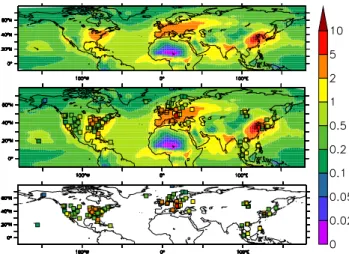
Fig. 6. Annual mean column tropospheric burden of the total
con-centration of (a) BC, (b) POM, (c) dust, (d) sea salt. The concen-tration of sea salt is calculated as the sum of sodium and chloride and bulk sea salt concentrations. All units are in mg m−2.
4.2.1 Bulk species: BC, POM, dust and sea spray Figures 6 shows the 2-year annual mean vertically integrated tropospheric burden of the bulk species simulated (summed over all modes, all model levels with pressure>150 hPa are assumed to be tropospheric). The burden of the species largely reflects the distribution of emissions; BC and POM concentrations are high over the biomass burning region of central Africa and South America, with additional maxima over India and China. Dust concentrations show the strong emission regions of Africa and Asia, and some intercontinen-tal transport including the outflow of Saharan dust over the Atlantic. In general the distribution of the species is simi-lar to that simulated using ECHAM-HAM (as shown in Stier et al., 2005, their Fig. 2).
The simulated annual mean concentration of BC, POM, dust and sea spray is compared to measurements in Fig. 8 and summarised in Table 3. Dust aerosol is well simulated (compared to the University of Miami data set) both close to and far from sources, although there is generally a low bias (AMR = 0.83, GMR = 0.58, PF = 42). Dust emissions have a large inter-annual variability thus it is advantageous to compare to datasets that span a number of years (as done here), but in these simulations we use offline dust emissions representative of the year 2000 thus we will underestimate the inter-annual variability in dust concentrations.
Table 3. Summary of the comparison of model data (2001 and
2002) to observations of bulk species (as shown in Fig. 8 with simulations performed using ISORROPIA and EQSAM3 to treat gas/aerosol partitioning). AMR is the arithmetic mean of the mod-elled values/the arithmetic mean of the observed values; GMR is the geometric mean of the modelled values/the geometric mean of the observed values; PF2 = Percentage of modelled points within a factor of two of the observations.
GMXe-ISORROPIA GMXe-EQSAM3
Species AMR GMR PF2 AMR GMR PF2
Dust 0.83 0.58 42.85 0.81 0.60 42.86
Sea Salt 1.15 1.95 61.76 1.08 1.82 61.76
BC 0.96 0.98 100.00 0.99 0.98 100.00
POM 1.46 1.31 91.67 1.48 1.33 83.30
future the good agreement between model and observations will be investigated further with comparison of a higher res-olution model to data taken from a wider range of environ-ments (including polluted regions and regions of biomass burning).
To compare with bulk sea spray observations, we sum the mass of Na+, Cl−and bulk sea spray to give a total sea spray concentration. Concentrations are well captured in marine regions although there is a slight high bias. In coastal regions sea salt concentrations are overestimated by up to an order of magnitude (overall, GMR = 1.94, PF2 = 62%). A similar bias was also noted in the ECHAM-HAM model (using online emissions), and Stier et al. (2005) suggest that it is due to artificial transport by averaging over large grid boxes, thus underestimating the sharp concentration gradients that occur in coastal regions.
In the simulations presented here, the hydrophilic coarse mode is assumed to have a geometric standard deviation (σ) of 2.2, this is larger than the σ used by Stier et al. (2005, σ= 2.0). The larger geometric standard deviation is chosen as it reduces the bias in sea spray concentrations in coastal regions, because the wider mode increases the rate of de-position due to both dry dede-position and sedimentation. The faster deposition leads to more realistic gradients in sea salt concentrations in coastal regions and improves comparison to observations.
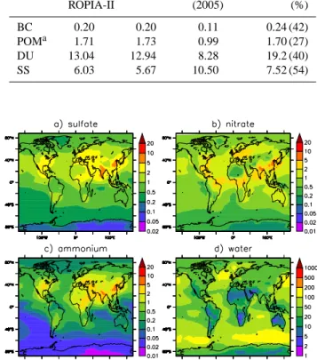
Table 4 summarises the budget of the bulk species com-pared to other studies. The simulated burdens in GMXe are within the range of the other models, with a simulated burden (in Tg) of 0.20 (BC), 1.71 (POM), 13.04 (Du) and 6.03 (SS). The BC burden is larger than that simulated in Stier et al. (2005), probably due to the assumption of 5 monolayers for the conversion of aerosol from hydrophobic to hydrophilic (cf., one monolayer in Stier et al., 2005), but it is closer to the AEROCOM medium value. The sea spray burden is to-wards the lower end of the range of AEROCOM estimates, but despite this the model tends to overestimate compared to observations.
Table 4. Budget of the bulk species compared to values reported
for the M7 within the ECHAM-HAM model (Stier et al., 2005) and the AEROCOM multi-model inter-comparison (Textor et al., 2006). The standard deviation of reported AEROCOM values is given in brackets.
Bulk GMXe GMXe Stier AEROCOM A
Species ISOR- EQSAM3 et al. (St. Dev.)
ROPIA-II (2005) (%)
BC 0.20 0.20 0.11 0.24 (42)
POMa 1.71 1.73 0.99 1.70 (27)
DU 13.04 12.94 8.28 19.2 (40)
SS 6.03 5.67 10.50 7.52 (54)
Fig. 7. Annual mean column tropospheric burden of the total
con-centration of (a) sulfate, (b) nitrate, (c) ammonium and (d) water. All units are in mg m−2.
4.2.2 Sulfate, ammonium and nitrate
Figure 7 shows the tropospheric column burden of the sul-fate, ammonium and nitrate aerosol. High concentrations (>1 mg(SO4) m−2) of sulfate aerosol occur over most
con-tinental regions in the Northern Hemisphere, apart from the less populated regions north of 50◦N, with concentrations of >2 mg (SO4) m−2) also common. The sulfate column
bur-den is at a maximum (>5 mg (SO4) m−2) over India and
eastern China. The column burden of sulfate is generally
≥0.2 mg (SO4) m−2, even over the remote ocean, arising
from the assumption that 5% of the sea spray mass flux is sul-fate. The burden of ammonium aerosol is largely restricted to continental regions with values of ≥1 mg (NH4) m−2
over most polluted continental regions, reducing to 0.2– 1 mg (NH4) m−2in the N Atlantic and other polluted marine
Table 5. Comparison of burdens with other studies. As HNO3concentrations above the troposphere contribute significantly to the global
burden, tropospheric only burdens are given in brackets. For GMXe the tropospheric value is defined as the burden in all model layers with at pressure>150 hPa.aEMAC only reports the sum of the gas + aerosol phase wet deposition, thus value for e.g. NH4+is the wet deposition
of ammonia+ammonium (same for HNO3and H2SO4). All units are Tg N (or S) yr−1.
GMXe GMXe Pye Bauer Feng and Rodriguez Liao
ISORROPIA-II EQSAM3 et al. et al. Penner Dabdub et al.
(2009) (2007) (2007) (2004) (2003)
Emissions
SO2 97.9 97.9 72.5 83.9 66.05
NH3 50.85 50.85 55.0 54.1 54.1 52.08
NOx 43.40 43.40 33.4 46.2 38.9 34.73 40.0
Burden
SO2 0.55 0.55 0.48 0.204
SO42− 0.53 0.51 0.28 0.56 0.703
NH3 0.16 0.19 0.17 0.084 0.192 0.19
NH4+ 0.21 0.20 0.24 0.27 0.29 0.045 0.26
HNO3 1.28 (0.55) 1.29 (0.58) 3.88 (0.37) (0.958) (0.28)
NO3− 0.13 0.11 0.35 0.52 0.16 0.417 0.18
Wet Deposition
SO2 5.08
SO42− 55.69a 53.87a 28.7 51.69
NH3 13.1 16.7
NH4+ 22.12a 22.35a 21.1 23.0 4.32
HNO3 16.9 3.97 8.4
NO3− 24.79a 24.46a 13.7 8.6 18.69 5.9
Dry Deposition
SO2 34.42 34.36 33.02
SO42− 4.86 4.86 4.52
NH3 19.14 19.48 15.4 29.35
NH4+ 0.65 0.63 2.8 0.2
HNO3 24.37 26.12 7.5 3.97 6.3
NO3− 1.78 1.73 3.0 1.11 7.7
The horizontal distribution of nitrate is generally similar to that of sulfate; nitrate is of a similar magnitude to sulfate in many polluted regions (e.g. East Asia, India and the east of North America), and it is at a maximum (>5 mg (NO3) m−2)
in the regions of India and eastern China where sulfate con-centrations are also high.
Table 5 summarises the budget of the sulfate/nitrate/ ammonium system in GMXe and compares it to that of other works which have treated nitrate. The first thing to note is that there is a large range in published burdens of aerosol, this can arise from the range in the treatments of the aerosol distribution e.g. if nitrate formation is permitted in the coarse mode, or if equilibrium is assumed, from different treatments of wet/dry deposition, and from different representations of gas-phase precursors and NOx emissions. The burden of
sulfate and ammonia simulated with GMXe falls within the range of other models, however the simulated nitrate burden of 0.13 Tg (N) of NO3 is a little below the range of other
models (0.16–0.52 Tg (N)).
Observed ( g m )
10 10
-2 -1 0 1 2
10 10 10
-3
m
Sea Spray Black = BC, Red = POM Mineral Dust
M
o
del ( g m )
10 10
-2 -1 0 2
1
10 10 10
-3
m
M
o
del ( g m )
10 10
-2 -1 0 2
1
10 10 10
-3
m
M
o
del ( g m )
10 10
-2 -1 0 1
10 10
-3
m
Observed ( g m )
10 10
-2 -1 0 1 2
10 10 10
-3
m Observed ( g m )
10 10
-2 -1 0 1
10 10
-3
m
Fig. 8. Annual mean aerosol concentrations compared to the
Fig. 9. (a) Top panel: simulated annual mean concentration of
sul-fate aerosol (µg (SO42−) m−3) for the year 2001. (b) Same as (a)
but with observations from the CASTNET, EMEP and EANET net-works over-plotted. Panel (c) shows the observations alone.
4.3 Comparison of simulated sulfate, nitrate and ammonium concentrations to large-scale observation networks
To evaluate the simulated concentrations of sulfate, nitrate and ammonium we compare to data gathered from a num-ber of large-scale monitoring networks. In this first section modelled concentrations are compared to observational data taken from the European Monitoring and Evaluation Pro-gramme network (EMEP), Clean Air Status and Trends NET-work (CASTNET, in North America), Interagency Monitor-ing of PROtected Visual Environments (IMPROVE, North America) and Acid Deposition Monitoring Network in East Asia (EANET). These networks combined give a reasonable coverage of some of the most populated regions in the North-ern Hemisphere.
The details of the evaluation are discussed in the following section. In the following section both the observations and the model results are from the years 2001 and 2002.
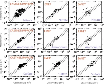
Figures 9 to 11 show the annual average surface concentra-tion of sulfate, ammonium and nitrate in the Northern Hemi-sphere for the year 2001. The top panel shows the model data only and in the middle and lower panels the average observation data for that year (2001) are over-plotted. The comparison to the continental observations is summarised in Fig. 12, which shows annual mean values for each simulation year (2001 to 2002) plotted against point observations for that year. The dotted lines are the 1:2 and 2:1 lines. Table 6 summarises the bias between the model and the observations from the large scale monitoring networks.
Fig. 10. Same as Fig. 9 but for ammonium aerosol
(µg (NH4+) m−3).
Fig. 11. Same as Fig. 9 but for nitrate aerosol (µg (NO32−) m−3).
4.3.1 Sulfate
In general the model captures the distribution and magnitude of the sulfate concentration well; the maxima occur over the highly populated regions of each continent, regions which are well known to have high aerosol loading. Sulfate has a high concentration also over the Mediterranean and Saudi Arabia, much of this sulfate arises from export from Europe where emission of SO2is high. Stier et al. (2005) note that
the dry deposition velocity of SO2 may be underestimated
(compared to other studies) by the dry deposition scheme of Ganzeveld et al. (1998) that is used (in different implementa-tions) in both ECHAM-HAM and GMXe, thus the modelled burden of sulfate in this region may be overestimated.
Observed ( g m ) Observed ( g m )m -3 Observed ( g m )m -3 m -3 Nitrate
EANET
Observed ( g m )m -3 Observed ( g m )m -3 Observed ( g m )m -3
Nitrate Nitrate
Ammonium Ammonium Ammonium
Sulfate Sulfate Sulfate
CASTNET/IMPROVE
CASTNET/IMPROVE
CASTNET/IMPROVE
EMEP
EMEP EMEP
EANET EANET
M
o
del ( g m )
-3
m
M
o
del ( g m )
-3
m
M
o
del ( g m )
-3
m
Fig. 12. Observed and modelled (with ISORROPIA-II) annual average concentrations (in µg m−3) for the year 2001 of nitrate (top row), ammonium (middle) and sulfate (lowest row) compared to observational data. Left column: CASTNET (star) and IMPROVE (triangle); middle column: EMEP; right column: EANET. Dashed lines indicate the 1:2 and 2:1 ratios.
Table 6. Summary of the comparison of model data to observations taken from the EMEP (Europe), CASTNET (North America) and
EANET (Asia) networks (simulations performed using ISORROPIA-II and EQSAM3 are shown). AMR is the arithmetic mean of the modelled values/the arithmetic mean of the observed values; GMR is the geometric mean of the modelled values/the geometric mean of the observed values; PF2 = Percentage of modelled points within a factor of two of the observations.
GMXe-ISORROPIA GMXe-EQSAM3
Site Species AMR GMR PF2 AMR GMR PF2
CASTNET SO42− 0.81 0.92 85.1 0.79 0.89 91.2
CASTNET NH4+ 1.02 1.01 92.4 0.72 0.80 91.1
CASTNET NO3− 2.11 2.28 43.7 0.93 1.17 55.0
IMPROVE SO4− 1.26 1.48 68.0 1.17 1.41 70.9
IMPROVE NO3− 2.29 2.01 43.7 1.49 1.49 53.4
EMEP SO42− 1.25 1.19 82.7 1.24 1.18 82.7
EMEP NH4+ 1.31 1.01 68.4 0.90 0.69 68.4
EMEP NO3− 1.47 1.66 50.0 0.67 0.91 73.1
EANET SO42− 1.16 1.06 64.7 1.13 1.01 58.8
EANET NH4+ 1.21 0.90 58.8 0.92 0.83 76.5
EANET NO3− 2.76 2.55 41.2 1.43 1.58 52.9
well captured with 64.7% of predictions within a factor of 2 of observations. This is expected to be related to the large uncertainties in emission estimates in the region.
4.3.2 Ammonium
The distribution of ammonium aerosol is concentrated in continental regions where concentrations of ammonia are high, e.g. China and India (Clarisse et al., 2009) and where there is an abundant supply of acidic gases (e.g. H2SO4and
HNO3). Ammonium concentrations show very good
com-parison to observations in North America with both model and observations predicting values of 0.1–1.0 µg (NH4) m−3
in the west of the country and ≥1.0 µg (NH4) m−3 in the
4.3.3 Nitrate
Like sulfate, nitrate concentrations peak in the populated re-gions of North America, Europe and Asia where precursor emissions are high, but elevated nitrate concentrations are also found in coastal regions close to the populated regions. This happens because in inland continental regions the for-mation of aerosol nitrate is limited by the availability of am-monium. As ammonium sulfate is formed preferentially over ammonium nitrate, the latter only forms in inland regions if there is excess cations e.g. ammonia or the cations present in mineral dust available after all the sulfate has been neu-tralised. This is not the case in coastal and marine regions where nitrate can enter the aerosol phase using sodium (and not ammonium) as a corresponding cation, resulting in the expulsion of HCl and facilitating the formation of aerosol ni-trate. Thus concentrations of nitrate in coastal regions can be significant (e.g. Yeatman et al., 2001).
Nitrate concentrations in Europe are reasonably well cap-tured but in North America there is an overestimation of nitrate compared to observations (by approximately a fac-tor of 2.0). Part of this overestimation is likely to arise from measurement biases in the IMPROVE and CASTNET data sets. The nitrate concentrations observed by the CAST-NET network are known to have a low bias, especially in warm dry conditions, as nitrate can evaporate from the fil-ters when temperatures are high (summarised in Ames and Malm, 2001). The IMPROVE network does not efficiently sample aerosol>2.5 µm aerodynamic diameter due to the in-let type (Ames and Malm, 2001), and thus will underestimate total nitrate, which is particularly important in regions where a large fraction of the nitrate is in the coarse mode.
Although these sampling issues may explain part of the bias, it is likely that GMXe overestimates the concentration of nitrate aerosol in coastal regions because of the overesti-mation of sea spray aerosol in these regions; the overabun-dance of sodium results in an overestimation of aerosol ni-trate if HNO3concentrations are significant. The choice of a
largerσfor the coarse hydrophilic mode (Sect. 4.2.1) reduces the bias in sea salt concentrations and improves the compar-ison of modelled nitrate to observations in these regions.
An additional possible cause of bias in the simulated ni-trate concentrations comes from the concentrations of the gas phase precursors. Estimates of global NOxemissions are
un-certain (e.g. Konovalov et al., 2008; Han et al., 2009) and these uncertainties (along with uncertainties in the deposition rate of gas phase precursors) add to the potential for biases in the gas phase precursor fields. The simulated fields of HNO3
and NO in ECHAM/MESSy were evaluated in J¨ockel et al. (2006) and Tost et al. (2007a) examined the wet deposition of nitrate and found the model simulated deposition fluxes to be in good agreement with observations.
In east Asia, the predicted mean value of nitrate is well captured but there is considerable scatter caused by an over-estimation of nitrate concentrations at marine influenced sites
10 10
-2 -1 0 2
1
10 10 10
M
o
del ( g m )
10 10
-2 0 1
10 10 10
Observations ( g m )
10 10
-2 -1 0 1 2
10 10 10
10 10
-2 -1 0 1 2
10 10 10
10 10
-2 -1 0 2
1
10 10 10
10 10
-2 -1 0 2
1
10 10 10
Sulfate Ammonium Nitrate
-3 m
-3
Observations ( g m )m -3 Observations ( g m )m -3
m
2 -1
Fig. 13. Simulated concentration of sulfate, ammonium and nitrate
aerosol for the year 2001 (star) and 2002 (triangle) compared to AMS data summarised by Zhang et al. (2007).
between China and Japan and an underestimation at some more remote sites. We note that in general the model tends to have difficulties in East Asia, probably due to the com-plexity of the meteorology and the large uncertainties in the emissions in this region.
4.4 Aerosol mass spectrometer data
In addition to long term observational data sets it is also use-ful to compare to data gathered in short term field campaigns. Zhang et al. (2007) summarised aerosol mass spectrometers (AMS) observations gathered in a range of field campaigns in North America, Europe and East Asia which were performed between 2000 and 2006. In Fig. 13 we compare GMXe fields to this observational database. To capture any seasonal de-pendence we extract the model data for the months of the different campaigns. As the measurements are of sub-micron mass, in this comparison we consider only the mass that is<1 µm diameter (calculated from the average size of the aerosol at the measurement locations). We use model data representative of 2001 and 2002, although the field campaign data was taken over a range of different years.
10 5 2 1 0.5 0.2 0.1 0.05 0.02
10 10
-2 -1 0 2
1
10 10 10
M
o
del ( g m )
-3
m
10-2 10-1 100 101 102
Observations ( g m )m -3
Nitrate
10 5 2 1 0.5 0.2 0.1 0.05 0.02
10 10
-2 -1 0 2
1
10 10 10
M
o
del ( g m )
-3
m
10-2 10-1 100 101 102
Observations ( g m )m -3
Sulfate Nitrate
Sulfate
Fig. 14. Comparison of modelled data to data collected by
AE-ROCE. Maps show surface concentrations of nitrate (top) and sul-fate (bottom) for the year 2002 simulated using ISORROPIA-II with observed values overplotted (squares). Scatter plots show the comparison of modelled vales to AEROCE data for nitrate (top) and sulfate (bottom) for the year 2001 (triangles) and 2002 (stars). All units are µg m−3.
4.5 Marine regions: AEROCE data
The AEROCOM inter-comparison project has made avail-able data from the Atmosphere/Ocean Chemistry Experi-ment (AEROCE), SEAREX and DOE projects (J. Prospero, personal communication, 2009, for an overview see: http:// www.igac.noaa.gov/newsletter/24/aeroce.php). The data set consists of measurement data taken from remote marine re-gions during the 1980s and 1990s. These data are multi-annual data which have been averaged to provide a clima-tology of marine aerosol observations. In Fig. 14 we show comparison of simulated concentrations of sulfate and nitrate compared to the observed data. The sulfate data observed is reported as non-sea salt sulfate but we compare to total sul-fate simulated by the model, thus simulated concentrations may be biased high.
Both the distribution and the magnitude of the observed values are captured well by the model; PF2 = 82% for sulfate and 96% of nitrate, with a GMR of 1.01 and 1.21, respec-tively. The good agreement between simulated and observed nitrate implies that the partitioning of HNO3to the sea spray
aerosol is well represented in the model. Sulfate values are well simulated at polluted sites but are overestimated in very remote marine regions. As the geographical distribution of sulfate precursor emissions has changed significantly since the 1980s, a perfect agreement between model and observa-tions is not expected, however, this change in the distribution of emissions is less important for remote marine locations where the AEROCE data is concentrated.
4.6 Aerosol optical depth
Aerosol optical depth (AOD) is a useful diagnostic for val-idating global and regional aerosol models as not only it is one of the most important diagnostics for climate forcing, but it is also relatively easy to evaluate as both local and global measurements of AOD are available. A new sub-model is currently being developed for use in the EMAC model (AEROPT), this submodel will calculate AOD in a sophisticated manner, once complete it is a straightforward task to couple the aerosol fields simulated with GMXe to the new submodel. However, development and evaluation of AOD parametrisation scheme is a non-trivial task and the submodel is not yet fully developed.
For evaluation purposes, we use a simplified treatment of AOD, based on the parametrisation of Kiehl and Briegleb (1993):
AOD(λ)=f (RH,λ)B(λ)α (2)
where AOD(λ) is the optical depth at the reference wave-length (λ) and B(λ) is the mass extinction coefficient (m2g−2). For the latter, we take mean values of 5 for sulfate, nitrate and ammonium (Jeuken et al., 2001); 9 for BC; and 4 for POM (Liousse et al., 1996) and 3 for sea spray (Kinne et al., 2006). The effect of variations in relative humidity (RH) on AOD is taken into account in the termf (RH,λ), we approximate this effect using the parametrisation of Veefkind (1999); Tsigaridis et al. (2005), which relates f (RH,λ)to RH using a polynomial fit which they derived from observa-tional data. This calculation of AOD is taken from Jeuken et al. (2001); Tsigaridis et al. (2005, 2006). Although we acknowledge that this is a simplified treatment of aerosol optical depth, it should suffice for a first evaluation with remotely-sensed AOD values. A more detailed analysis of aerosol optical depth simulated with GMXe will be presented in future work.
0.75 0.50 0.40 0.30 0.25 0.15 0.10 0.010.05 0.20
0.75 0.50 0.40 0.30 0.25 0.15 0.10
0.010.05 0.20
0.00
Observed
0.20 0.40 0.60 0.80
M
o
del
0.00 0.20 0.40 0.60 0.80
Fig. 15. (a) Annual mean AOD modelled with GMXe for the
year 2001, over-plotted are annual mean measurements from the AERONET network (2001), (b) summary of the comparison be-tween GMXe and AERONET, black points are monthly mean and
red are annual mean (r2= 0.51). (c) Annual mean AOD from
MODIS for 2001.
The scatter plot shows that most (92%) simulated AOD values are within a factor of two of the AERONET obser-vations, however despite the generally good agreement with observations there is still a lot of scatter in the comparison, particularaly in the monthly mean data, this implies that the seasonal cycle of the AOD may not always be well cap-tured. This will be investigated further with the AEROPT submodel, when the submodel development is complete.
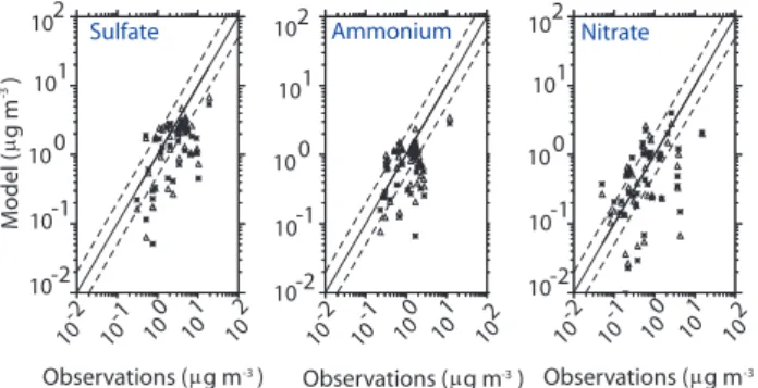
4.7 Sensitivity to the choice of partitioning model
The model framework of GMXe allows the user to choose between two gas/aerosol partitioning schemes. In all the dis-cussion so far the ISORROPIA-II scheme has been used. To demonstrate the sensitivity of the simulated species to the choice of partitioning model, Fig. 16 shows the comparison of fields simulated using the EQSAM3 treatment of parti-tioning with observations from the CASTNET/EMEP and EANET networks (comparable to Fig. 12 for ISORROPIA-II). In addition, Table 6 summarises the bias between model and the large-scale observation networks when EQSAM3 is used.
Nitrate concentrations are most sensitive to the choice of partitioning model; particularly in North America where ni-trate loadings are lower using EQSAM3 (and in better
agree-ment with observations). East Asian concentrations are still poorly captured, with a smaller high bias (GMR = 1.58), but with a very large amount of scatter. When EQSAM3 is used, GMXe tends to underestimate ammonium tions (GMR = 0.69 to 0.83) particularly at low concentra-tions. In contrast ISORROPIA-II, shows no consistent bias in ammonia concentrations (GMR = 0.8–1.01). Sulfate concen-trations are little affected by the choice of partitioning mod-els as both ISORROPIA-II and EQSAM3 assume that upon condensation sulfate remains in the aerosol phase.
The concentrations of the “bulk” species are also largely insensitive to the choice of partitioning model (Table 4, col-umn 2), this is to be expected as the only changes would come from (i) changes in the particle ageing due to different partitioning of the semi-volatile species on the bulk species, or (ii) changes in aerosol water uptake. The sensitivity of the simulated aerosol water to the choice of partitioning models is summarised in Table 7, which shows the calculated an-nual mean hygroscopic growth factor (GF = wet radius/dry radius) for each mode. The GF of the different modes reflects the change in composition with size: the Aitken mode has a large percentage mass of hydrophobic BC and POM (as this is the size where these species are emitted) and thus has the lowest GF. BC/POM are less dominant in the accumulation mode as condensed sulfate and nitrate and primary sea spray aerosol add mass (reducing the hydrophobic mass fraction), thus the GF is larger. The coarse mode has the largest GF as the composition is dominated by the highly hydrophilic sea spray aerosol. Both ISORROPIA-II and EQSAM3 cap-ture this trend in GF and simulate similar global mean GFs (percentage difference≤6%). For both ISORROPIA-II and EQSAM3, the global distribution of GF is dominated by the distribution of relative humidity (not shown).
In summary, the choice of partitioning model has a small effect on the distribution of most aerosol species, the excep-tion is nitrate, the concentraexcep-tion of which is generally lower when EQSAM3 is used.
Observed ( g m )
Observed ( g m )m -3 Observed ( g m )m -3 m -3
Nitrate
EANET
Observed ( g m )m -3 Observed ( g m )m -3 Observed ( g m )m -3
Nitrate Nitrate
Ammonium Ammonium Ammonium
Sulfate Sulfate Sulfate
CASTNET/IMPROVE
CASTNET/IMPROVE
CASTNET/IMPROVE
EMEP
EMEP EMEP
EANET EANET
M
o
del ( g m )
-3
m
M
o
del ( g m )
-3
m
M
o
del ( g m )
-3
m
Fig. 16. Observed and modelled (with EQSAM3) annual average concentrations (in µg m−3) for the year 2001 of nitrate (top row), ammo-nium (middle) and sulfate (lowest row) compared to observational data. Left column: CASTNET (star) and IMPROVE (triangle); middle column: EMEP; right column: EANET. Dashed lines indicate the 1:2 and 2:1 ratios.
Table 7. Summary of the annual mean hygroscopic growth factors (GF = wet radius/dry radius) for the simulation using ISORROPIA-II and
EQSAM3. Analysis considers (i) the surface layer only and (ii) all vertical levels.
ISORROPIA-II EQSAM3
Mode Mean St. Dev. Mean St. Dev. % Difference
Surface
Aitken 1.25 0.05 1.18 0.03 5.60
Accumulation 1.67 0.18 1.70 0.18 −1.80
Coarse 1.82 0.20 1.87 0.19 −2.75
Whole atmosphere
Aitken 1.26 0.08 1.20 0.05 4.76
Accumulation 1.37 0.17 1.35 0.16 1.46
Coarse 1.48 0.25 1.46 0.24 1.35
5 Conclusions
This paper has introduced a newly developed aerosol sub-model which has been implemented and tested within the EMAC general circulation model. The treatment of aerosol microphysics in the submodel is similar to that of the M7 model (Vignati et al., 2004), but a number of new develop-ments have been made:
– The microphysics code has been extended to allow the simulation of an increased and varied number of aerosol species; in addition to the five species (SS, POM, BC,
Du and SO42−) treated by M7, GMXe can also treat
NO3−, NH4+, Na+, Cl−, Ca2+, Mg2+, K+and
poten-tially more (including organics).