www.nat-hazards-earth-syst-sci.net/11/2981/2011/ doi:10.5194/nhess-11-2981-2011
© Author(s) 2011. CC Attribution 3.0 License.
and Earth
System Sciences
Evaluating sources of uncertainty in modelling the impact of
probabilistic climate change on sub-arctic palsa mires
S. Fronzek1, T. R. Carter1, and M. Luoto2
1Finnish Environment Institute (SYKE), Helsinki, Finland
2Department of Geosciences and Geography, University of Helsinki, Finland
Received: 12 July 2011 – Revised: 22 September 2011 – Accepted: 25 September 2011 – Published: 8 November 2011
Abstract. We present an analysis of different sources of impact model uncertainty and combine this with proba-bilistic projections of climate change. Climatic envelope models describing the spatial distribution of palsa mires (mire complexes with permafrost peat hummocks) in north-ern Fennoscandia were calibrated for three baseline periods, eight state-of-the-art modelling techniques and 25 versions sampling the parameter uncertainty of each technique – a to-tal of 600 models. The sensitivity of these models to changes in temperature and precipitation was analysed to construct impact response surfaces. These were used to assess the be-haviour of models when extrapolated into changed climate conditions, so that new criteria, in addition to conventional model evaluation statistics, could be defined for determining model reliability. Impact response surfaces were also com-bined with climate change projections to estimate the risk of areas suitable for palsas disappearing during the 21st cen-tury. Structural differences in impact models appeared to be a major source of uncertainty, with 69 % of the models giving implausible projections. Generalized additive mod-elling (GAM) was judged to be the most reliable technique for model extrapolation. Using GAM, it was estimated as
very likely(>90 % probability) that the area suitable for
pal-sas is reduced to less than half the baseline area by the period 2030–2049 and as likely (>66 % probability) that the
en-tire area becomes unsuitable by 2080–2099 (A1B emission scenario). The risk of total loss of palsa area was reduced for a mitigation scenario under which global warming was constrained to below 2◦C relative to pre-industrial climate,
although it too implied a considerable reduction in area suit-able for palsas.
Correspondence to:S. Fronzek ([email protected])
1 Introduction
Recent developments in climate modelling have made it possible to express projections of regional climate change for Europe probabilistically quantifying various aspects of climate modelling uncertainty (R¨ais¨anen and Ruokolainen, 2006; Murphy et al., 2007; D´equ´e and Somot, 2010; also see the review of Christensen et al., 2007, pages 921–925). These typically involve large ensembles of climate model simulations combined with some statistical analysis. Prob-ability distributions are fitted for projected changes in key climate variables. The construction of such probabilistic pro-jections of climate change was one of the main objectives of the EU-FP 6 ENSEMBLES project (van der Linden and Mitchell, 2009).
An alternative approach for assessing impact risks is to construct impact response surfaces from a sensitivity study of the impact model with respect to key climatic variables and to superimpose probabilistic climate change projections onto these (Jones, 2000a, b; Luo et al., 2007; Fronzek et al., 2010). The risk of exceeding critical impact thresholds can then be quantified by calculating the proportion of ensem-ble members lying above the threshold. In an earlier paper, we presented an example of this approach with a climatic envelope model, using a probabilistic projection of climate change constructed by re-sampling an ensemble of General Circulation Model (GCM) runs (Fronzek et al., 2010). How-ever, impact model uncertainty was not quantified in that study.
Model uncertainty can be grouped into three different types: (1) uncertainty due to the structure of the model, (2) the parameter uncertainty of a single model, and (3) un-certainty of the initial conditions (Thuiller et al., 2009). Cli-matic envelope techniques have been applied widely to as-sess the impact of climate change on the spatial patterns of biodiversity and many aspects of their uncertainty have been discussed (Heikkinen et al., 2006; Jeschke and Strayer, 2008). It has also been suggested to quantify the uncertainty of envelope models by using large ensembles of impact mod-els (Ara´ujo and New, 2007; Thuiller et al., 2009). However, the application of envelope models with climate change sce-narios often implies model extrapolations to climatic condi-tions that lie outside the range of values with which models have been calibrated. Moreover, testing the validity of ex-trapolations is difficult, as the response of future biodiversity range shifts cannot be measured (Ara´ujo et al., 2005). For this reason, in this paper we advocate a rigorous testing of the sensitivity of envelope models to evaluate the robustness and plausibility of extrapolations.
We present an analysis that attempts to quantify impact model uncertainty, or at least some aspects of it, and com-bines this with probabilistic projections of climate change. We demonstrate this in a case study of sub-arctic palsa mires. Palsas are peat mounds with an ice core that is frozen all year round (Sepp¨al¨a, 2011). They are located at the outer limit of the permafrost zone in sub-arctic regions, and hence are sen-sitive to even small changes in climate. Luoto et al. (2004a) and Fronzek et al. (2006) presented statistical climatic en-velope models of the spatial distribution of palsa mires in northern Fennoscandia. One of these models was applied with probabilistic climate change projections derived from an ensemble of 21 General Circulation Models (GCMs), us-ing the impact response surface approach to estimate the risk of palsa mire loss during the 21st century (Fronzek et al., 2010). However, the uncertainty of the impact model was not assessed. This paper extends the previous analysis and has the following four objectives:
1. to quantify the uncertainties of climatic envelope mod-els for palsa mires, where possible probabilistically; 2. to evaluate the robustness and plausibility of model
ex-trapolations;
3. to apply the impact models with more comprehen-sive probabilistic projections of regional climate change generated in the ENSEMBLES project for the SRES A1B (moderate emissions) scenario, based on GCM simulations and observed constraints; and
4. to compare these probabilistic results with determin-istic scenarios from an ensemble of atmosphere-ocean GCM simulations for the E1 stabilization scenario and the SRES A1B scenario, in order to gain insight on the effectiveness of mitigation policy in reducing the risk of disappearance of European palsa mires.
2 Material and methods
2.1 Ensemble of palsa mire distribution models
The presence or absence of palsa mires has been mapped using geomorphological and topographical maps and aerial photography (Luoto et al., 2004a; updated) onto a regu-lar grid with 10′×10′ spacing for Fennoscandia north of
the Arctic Circle (Fig. 1). Gridded monthly mean temper-ature and annual precipitation observations for the period 1951–2000 were extracted from the Climatic Research Unit TS 1.2 dataset at the same 10′×10′resolution (New et al.,
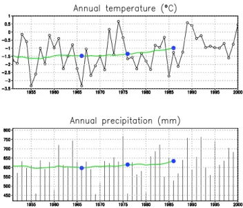
2002; Mitchell et al., 2004). Period averages were calcu-lated for three 30 yr baseline periods, 1951–1980, 1961– 1990 and 1971–2000, offering a range of long-term refer-ence climates. The 1951–1980 period was coolest and had the smallest annual precipitation, while 1971–2000 was the warmest and wettest of the three periods (Fig. 2). The follow-ing climate parameters were then derived for the three 30 yr mean periods: Thawing degree days (TDD), freezing degree days (FDD), continentality (CONT) and annual precipitation (APREC). TDD and FDD, defined as the accumulated sum of daily mean temperatures above (TDD) or below (FDD) 0◦C, have been calculated from monthly mean temperatures
using a method suggested by Kauppi and Posch (1985). This required information on the standard deviation of daily mean temperature around the monthly mean, for which a gridded dataset interpolated from station data was used (Fronzek and Carter, 2007). CONT was defined as the difference between the maximum and minimum of the mean monthly tempera-tures.
Fig. 1. Map of the study area showing the location of palsas in Northern Fennoscandia (Luoto et al. 2004, updated).
tree analysis (CTA), mixture discriminant analysis (MDA), artificial neural network (ANN), random forest (RF), and generalized boosting methods (GBM) (Table 1). Marmion et al. (2008) classify these methods into regression methods (GLM, GAM, MARS), classification methods (CTA, MDA) and machine learning methods (ANN, RF, GBM). RF and GBM use a large number of regression trees and could there-fore also be described as classification methods. The models give values on a continuous scale between 0 and 1; to con-vert these into predicted presences or absences, a threshold was determined by minimizing the difference between cor-rect presence and corcor-rect absence predictions.
For each of the 8 modelling techniques and each of the 3 baseline periods, we calibrated models by randomly split-ting the data into calibration and evaluation sets 25 times re-sulting in 8×3×25 = 600 models. The calibration data sets contained data from 70 % of the grid cells retaining the same ratio of palsa presences and absences as in the full data sets; the remaining 30 % of the grid cells were used as evalua-tion data sets. Although arbitrary, this proporevalua-tion is com-monly applied for the split-sampling of data (Ara´ujo et al., 2005). All subsequent analyses of uncertainty should thus be regarded as conditional on the 70:30 split, which was applied consistently for all models.
Fig. 2.Area-averages of annual mean temperature and precipitation
(black lines), running 30 yr-averages centred at their mid-yr (green lines) and period-averages for 1951–1980, 1961–1990 and 1971– 2000 (blue points) for the European land grid cell north of the Arctic Circle (66.5◦N) of the CRU TS 2.02 dataset.
This ensemble of palsa mire distribution models samples three sources of impact model uncertainty: (1) initial con-ditions, by relating the observed palsa distribution with cli-matic conditions for different baseline periods, (2) model structure, by employing alternative statistical techniques to quantify palsa-climate relationships, and (3) model parame-ters, by sampling across the distribution of parameter values obtained for a single modelling technique (Table 2).
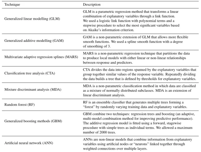
Table 1. Description of climatic envelope modelling techniques (based on Fronzek et al., 2006; Heikkinen et al., 2006; Elith et al., 2008; Marmion et al., 2008).
Technique Description
Generalized linear modelling (GLM)
GLM is a parametric regression method that transforms a linear combination of explanatory variables through a link function. We used a logistic link function with polynomial terms and a stepwise procedure to select the most significant variables based on Akaike’s information criterion.
Generalized additive modelling (GAM) GAM is a non-parametric extension of GLM that allows more flexiblesmooth functions. We used a spline smooth function with a degree of smoothing of 3.
Multivariate adaptive regression splines (MARS)
MARS is a non-parametric regression technique that partitions the data to produce local models with either linear or non-linear relationships between response and predictors.
Classification tree analysis (CTA) CTA divides the data into regions spanned by the explanatory variables thatgroup together similar values of the response variable. Repeatedly dividing the data builds a tree that is defined by thresholds for explanatory variables.
Mixture discriminant analysis (MDA)
MDA is a non-parametric classification method in which data are classified as a mixture of normally distributed subclasses. MDA is an extension of linear discriminant analysis.
Random forest (RF) RF is an ensemble classifier that generates multiple trees forming a “forest” by randomly varying training data and explanatory variables.
Generalized boosting methods (GBM)
GBM combine two techniques: regression trees and boosting (an adaptive, multi-model combination method for improving predictive performance). The additive regression model is fitted using a forward, stagewise procedure with simple trees as individual terms. We allowed a maximum number of 2000 trees.
Artificial neural network (ANN) ANNs are non-linear models that combine information from explanatoryvariables using artificial nodes or “neurons” linked together through weighted connections over multiple layers.
Since the model application is an extrapolation to cli-matic conditions outside the observations (see next sec-tion), two criteria were defined to distinguish models giving implausible results following extrapolation. A palsa model was regarded as implausible if, for no changes in precipitation:
1. increases (decreases) in suitability are projected for in-creased (dein-creased) temperature (tested at−1◦C, 0◦C,
1◦C, 3◦C and 5◦C); and
2. the area projected as suitable does not totally disappear for a warming of 6◦C relative to 1961–1990.
While essentially arbitrary, the first criterion can be justified by the thawing effect of warming – higher air temperatures will warm the soil and hence increase the risk of thawing permafrost. A warming of 6◦C, as used in the second crite-rion, would imply mean annual temperatures above 0◦C for the whole study area, which is generally believed to be well above the upper limit for palsas in Fennoscandia (Sepp¨al¨a, 2011). These are similar conditions as those found in central parts of Finland and Sweden for the period 1961–1990, and therefore far outside the current distribution of permafrost.
2.2 Impact response surfaces
Simulations with the 600 palsa models were conducted for each combination of temperature changes at 0.2◦C incre-ments between−3◦C and 6.8◦C and precipitation changes
at 5 % increments between−30 % and 50 % relative to the 1961–1990 baseline period, which was also the baseline period of one of the climate change datasets (see below). Since the explanatory variables of the palsa models require monthly mean temperature, we applied a seasonal pattern taken from the average of an ensemble of AOGCM simu-lations to scale the annual temperature change to monthly changes (Fronzek et al., 2010). A seasonal pattern of precip-itation changes was not needed as only annual precipprecip-itation was used as the explanatory variable in the palsa models.
Table 2.Sources of uncertainty in projecting climate change effects on palsa mires.
Source of uncertainty Sampling method Sample size
Palsa impact model 3×8×25 = 600
Initial conditions Sampling of the 30 yr baseline periods: 1951–1980, 1961–1990 and 1971–2000 3 Model structure Ensemble of climatic envelope techniques 8 Model parameters Sampling of random sub-sets of the data for calibration 25
Climate projection 10000 + 12
GCM structure Probabilistic projections of climate change
10 000 GCM parameters of climate change from a statistical emulator
Observed constraints based on GCM ensembles and observations for the SRES A1B emission scenario GCM structure/initial Individual GCM simulations (E1
12 conditions stabilization and SRES A1B)
0 2 4 6 8 10 12
0 10 20 30 40 50
T ( C)
P
-c
han
ge (
%
)
<95% <75% <50% <25% Grand ensemble, A1B
GCMs, A1B GCMs, E1
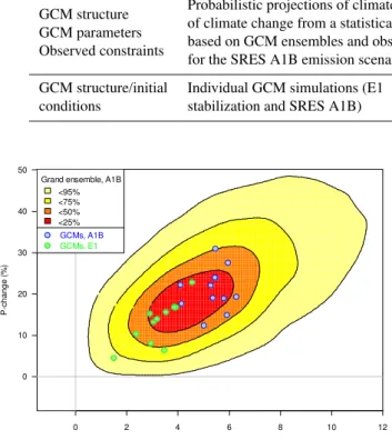
Fig. 3. Changes from 1961-1990 to 2080–2099 in annual mean
temperature (◦C) and precipitation (%) over northern Lapland for the Grand Ensemble probabilistic projection (Harris et al., 2010) and an ensemble of GCM simulations for the E1 mitigation and SRES A1B scenarios (Johns et al., 2011). Probabilities are depicted as the percentage of projections enclosed within coloured zones.
was assumed to be constant outside the range of values for which the sensitivity of the palsa models has been calculated. 2.3 Probabilistic climate projections and the risk of
palsa disappearance
The impact response surfaces were overlaid with projections of 21st century climate change to estimate future impacts on palsa suitability. Two datasets describing changes in an-nual mean temperature and anan-nual precipitation for north-ern Fennoscandia relative to the period 1961–1990 were ob-tained from the ENSEMBLES project (Fig. 3):
1. The “Grand Ensemble”, which describes joint proba-bilities of annual mean temperature and precipitation
changes for nine 20 yr periods during the 21st century (2000–2019, 2010–2029; 2080–2099) for the SRES A1B forcing scenario (Harris et al., 2010). This dataset combines information from perturbed physics ensem-bles, multi-model ensembles and observational con-straints, and quantifies uncertainties in the leading phys-ical, chemical and biological feedbacks. The data are available as joint frequency distributions with a sample size of 10 000.
2. Changes in temperature and precipitation extracted from 12 simulations of the E1 mitigation and the A1B non-mitigation scenarios with seven Earth System Mod-els and GCMs (Johns et al., 2011). Both emission scenarios were quantified with the IMAGE 2.4 inte-grated assessment model (van Vuuren et al., 2007). E1 is an aggressive mitigation scenario aimed at stabiliz-ing global warmstabiliz-ing below 2◦C relative to pre-industrial
levels (Lowe et al., 2009). The A1B simulations with the same climate models allow an evaluation of the im-pact avoided by the E1 scenario. The quantification of A1B used here slightly differs from the SRES A1B marker scenario which was quantified with a different integrated assessment model (Naki´cenovi´c et al., 2000). Simulated changes were obtained for the periods 2030– 2049 and 2080-2099.
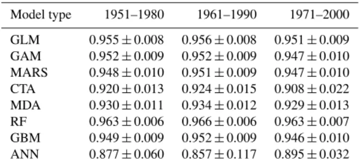
Table 3.Mean and standard deviation of the AUC evaluation statis-tics of the 25-member ensemble of palsa models for three calibra-tion time periods.
Model type 1951–1980 1961–1990 1971–2000 GLM 0.955±0.008 0.956±0.008 0.951±0.009 GAM 0.952±0.009 0.952±0.009 0.947±0.010 MARS 0.948±0.010 0.951±0.009 0.947±0.010 CTA 0.920±0.013 0.924±0.015 0.908±0.022 MDA 0.930±0.011 0.934±0.012 0.929±0.013 RF 0.963±0.006 0.966±0.006 0.963±0.007 GBM 0.949±0.009 0.952±0.009 0.946±0.010 ANN 0.877±0.060 0.857±0.117 0.895±0.032
3 Results
3.1 Model performance under baseline conditions Descriptive statistics for the 600 climatic envelope models are presented in Table 3. Nearly all models had AUC val-ues greater than 0.9 for the evaluation data sets, indicating excellent model agreement, the exceptions being versions of the ANN and CTA models. 36 of the 75 ANN models had AUC values below 0.9, with two models showing values be-low or equal to 0.5, indicating model performance no better than chance. These two models also had Kappa coefficients of 0, indicating model failure. Eight of the 75 CTA mod-els had AUC values below 0.9. ANN modmod-els had the largest variability in model performance.
RF models consistently had the highest AUC values ahead of GLM and GAM. The ratio of AUC values between eval-uation and calibration data sets was highest for GLM and GAM (average of 0.997 over all 75 ensemble members) and lowest for CTA (0.955) and RF (0.964). Similar results were achieved for the ratio of Kappa coefficients between evalu-ation and calibrevalu-ation datasets, which ranged between 0.978 for the ensemble averages of GLM and GAM to 0.774 for CTA.
GAM was the only technique for which all models ful-filled the two plausibility criteria for extrapolating to cli-matic conditions outside the range of calibration data; GLM fulfilled these criteria in all but one of the 75 models (Ta-ble 4). Decreases in area suita(Ta-ble for palsas with warming were projected for nearly all CTA, RF and GBM models and the majority of ANN models, whereas all MDA and nearly all MARS models failed this criterion. The total disappear-ance of area suitable for palsas for a warming of 6◦C was
projected by only a few MARS, CTA, MDA and RF models and by none of the GBM models. Altogether, 185 of the 600 models fulfilled both plausibility criteria.
3.2 Model behaviour under climate change
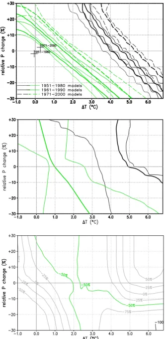
Impact response surfaces were constructed to examine the behaviour of each model under climate change. The full set (25 versions of all eight model techniques for three calibra-tion periods) is presented in Appendix A. Here we use se-lected examples to illustrate notable characteristics of model response.
Impact response surfaces for GAM and ANN models ful-filling the plausibility criteria are shown in Fig. 4a, b. The en-semble average of GAM calibrated for the 1961–1990 base-line period projects the total disappearance of area suitable for palsas with a warming of 4.5◦C, and the loss of half of
the area under a warming of 1.5◦C assuming no change in
precipitation (Fig. 4a). Increases in precipitation enhance the decline of suitability; hence the warming required for total or 50 % disappearance is smaller than that estimated without precipitation changes. The parameter uncertainty of GAM models gave a relatively narrow range of ca. 0.5◦C for the curves describing the palsa loss with ranges becoming wider for precipitation changes larger than±10 %.
ANN models gave a much wider range of projections than GAM, even excluding those models not fulfilling the plausibility criteria (Fig. 4b). The 11-member ensemble av-erage of ANN models projected the loss of half the palsa area for 1◦C warming and the total loss of palsa area for 4.9◦C
warming. Some other models resulted in more complex im-pact response surfaces, sometimes with non-monotonic rela-tionships of palsa change with warming. One such example was a CTA ensemble member for which a warming of up to 2◦C resulted in decreases in area suitable for palsas, but
additional warming produced a reversal in response towards increased suitability (Fig. 4c). GLM produced impact re-sponse surfaces with small variations similar to GAM, while GBM, RF and CTA also resulted in relatively small ranges (not shown), although most of these models did not fulfil the criterion of projecting total palsa loss for a large amount of warming (cf. Table 4). The response surfaces of the MARS and MDA models showed a very large variation, and most of these in any case failed the plausibility criteria.
GAM impact response surfaces for models calibrated with 1951–1980 (1971–2000) climate were shifted towards pro-jecting palsa area loss with less (more) warming and precipi-tation increases relative to the period 1961–1990, and largely retained the shape of the 1961–1990 impact response sur-faces (Fig. 4a). This largely reflects the observed trends in temperature and precipitation between the three calibration periods (cf. Fig. 2).
Table 4. Percentage of palsa models simulating decreases in palsa suitability with increased temperature and the total disappearance with 6◦C warming relative to 1961–1990 for three calibration time periods.
Complete loss of palsa suitability
Model type Decreased palsa suitability with warming with 6◦C warming Both criteria satisfied 1951–1980 1961–1990 1971–2000 1951–1980 1961–1990 1971–2000 All periods
GLM 100 100 96 100 100 100 99
GAM 100 100 100 100 100 100 100
MARS 4 0 8 4 0 0 1
CTA 96 88 72 4 0 4 3
MDA 0 0 0 8 4 0 0
RF 88 44 44 12 0 4 5
GBM 100 96 100 0 0 0 0
ANN 56 64 72 44 48 36 39
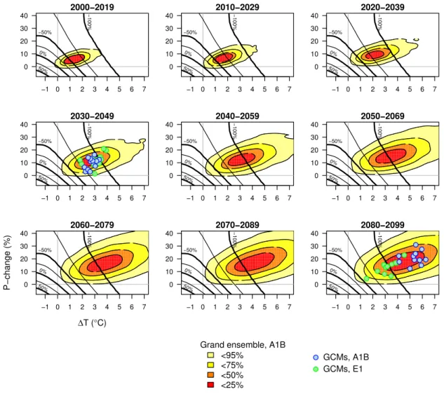
migrated across the threshold of total palsa loss for periods further in the future (Fig. 5). By the end of the 21st century, only a small fraction of the distribution remained below the impact threshold for 50 % loss of suitable area (Fig. 5, bot-tom row right).
The distribution of changes for the E1 mitigation scenario ensemble differed little from that of the non-mitigation A1B ensemble for the period 2030–2049, with most simulations resulting in 75 % to 100 % of the palsa area becoming un-suitable (Fig. 5, centre row left). In contrast, by 2080–2099, the A1B points have all crossed the impact threshold of total palsa loss, whereas more than half of the E1 ensemble mem-bers projected that some areas would remain suitable for pal-sas (Fig. 5, bottom row right). Three E1 simulations even showed slightly cooler conditions at the end of the 21st cen-tury compared to the 2030–2049 period, implying reversion of some previously unsuitable palsa areas.
3.4 Uncertainties in risk estimates
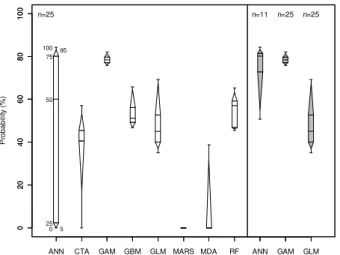
The estimated risk that all of the baseline palsa area becomes unsuitable by the end of the 21st century varies widely when a full ensemble of models, including those not fulfilling the plausibility criteria, is applied (white boxes and whiskers in Fig. 6). For one model class, MARS, all models calibrated with 1961–1990 climate predicted a 0 % probability for this impact threshold; this was also the case for all but 3 of the 25 MDA models. The remaining six model types showed me-dian estimates of between 41 and 78 %. The total range was largest for ANN, one version of which also gave the highest risk of 84 %.
When only plausible models were considered, estimates of the risk of crossing the impact threshold for total area loss showed a much smaller range for ANN from 51 to 84 % (11 models) while the ranges for GAM and GLM (all 25 mod-els plausible) are unchanged (grey boxes and whiskers in Fig. 6). The medians of the three modelling techniques re-sulting in plausible models for the calibration period 1961– 1990, ANN, GAM and GLM, spanned a similar range of uncertainty as that described by the parameter uncertainty
across the GLM and ANN models, whereas the parameter uncertainty across the GAM models was much narrower.
The GAM model results were used to compare parameter uncertainties with initial condition uncertainties in estimates of risk (Appendix B describes how these sources of uncer-tainty were combined). The risk of total loss of suitable area for palsas increased throughout the 21st century from 0 % (0 % to 1 %; 90 % confidence intervals) in 2000–2019 to 78 % (68 % to 84 %) in 2080–2099 (Fig. 7). The risk of 50 % loss increased from 72 % (44 % to 92 %) in 2000–2019 to 100 % (99 % to 100 %) by 2080–2099, with all periods after 2020–2039 having median estimates above 95 %. The range of 25-model-averages for each of the three calibration peri-ods was wider than the range of risk estimates spanned by parameter uncertainty for a single calibration period (black points vs. grey boxplots in Fig. 7). Initial conditions, there-fore, had a greater contribution to the combined uncertainty of GAM models.
4 Discussion
4.1 Comparison of climatic envelope modelling techniques
Fig. 4. Impact response surfaces showing the combinations of changes in annual mean temperature and precipitation for which half (green lines) and all (black lines) of the simulated palsa area be-comes unsuitable relative to the simulated distribution for the 1961– 1990 baseline period. The thicker lines show values for ensemble averages of: (a)GAM models calibrated for three different base-line periods (25 ensemble members each), with observed tempera-ture changes relative to 1961–1990 also shown (crosses);(b)ANN models calibrated for the 1961–1990 baseline period (11 ensemble members);(c)a single CTA ensemble member. The thinner lines show the range for the ensembles.
of envelope modelling techniques (Thuiller, 2003; Marmion et al., 2009; Luoto et al., 2010), although other studies re-sulted in a different ranking of techniques (e.g. Jeschke and Strayer, 2008) and general conclusions about a specific tech-nique outperforming others are difficult to make. Jeschke and Strayer (2008) reviewed 12 studies reporting climatic enve-lope models of species ranges that also used a split-sampling method for evaluation; they reported an average value of 0.85±0.029 (SE) for AUC. The AUC statistics reported here (Table 3) out-perform many of these other studies, indicat-ing the high capability of palsa models to reproduce the ob-served spatial distribution. One possible explanation is that species distributions can be strongly affected by biotic and human factors, such as competition and land use, in addi-tion to abiotic determinants such as climate. Another reason is that the distribution of northern Fennoscandian palsas is delimited solely by an upper limit (i.e. their southern range margin where climatic conditions become too warm). There is no lower limit, since the continuous permafrost that would define this does not exist in the study area.
Despite the generally good evaluation results, there was a large variation when these models were applied to mod-ified climatic conditions, producing qualitatively different model outcomes. This demonstrates that the use of evalu-ation statistics calculated with split-sample data remains dif-ficult and does not necessarily indicate if a model can also be used for extrapolation in climate change studies. Some models resulted in rather complex impact response surfaces that showed a non-monotonic relationship with warming like that shown for one of the CTA ensemble members in Fig. 4c. The introduction of plausibility criteria, based on knowledge of the processes governing palsa formation and maintenance (albeit subjectively interpreted), provides one means of dis-carding models that appear to behave unrealistically. Over fitting can be seen as one possible explanation why some models did not perform as well as others in the stability and plausibility criteria (cf. Ara´ujo et al., 2005).
It is interesting to speculate on the potential for deploying plausibility criteria in other applications of climatic envelope models. For example, obvious thresholds in the relationship between distributions of plant, insect or bird species and cli-matic variables may not exist, or may depend on species traits that are poorly understood. The plausibility criteria defined in this study are therefore specific to the palsa distribution in northern Fennoscandia. Nevertheless, even if no clear thresholds are known, impact response surfaces could help to identify species distribution models that show an unrealis-tically complex response.
4.2 Uncertainty and probabilistic impacts on palsa mires
−1 0 1 2 3 4 5 6 7 0 10 20 30 40 2000−2019 −100% −50% 0% 50%
−1 0 1 2 3 4 5 6 7 0 10 20 30 40 2010−2029 −100% −50% 0% 50%
−1 0 1 2 3 4 5 6 7 0 10 20 30 40 2020−2039 −100% −50% 0% 50%
−1 0 1 2 3 4 5 6 7 0 10 20 30 40 2030−2049 −100% −50% 0% 50%
−1 0 1 2 3 4 5 6 7 0 10 20 30 40 2040−2059 −100% −50% 0% 50%
−1 0 1 2 3 4 5 6 7 0 10 20 30 40 2050−2069 −100% −50% 0% 50%
−1 0 1 2 3 4 5 6 7 0 10 20 30 40 2060−2079 ∆T (°C) P−change (%) −100% −50% 0% 50%
−1 0 1 2 3 4 5 6 7 0 10 20 30 40 2070−2089 −100% −50% 0% 50%
−1 0 1 2 3 4 5 6 7 0 10 20 30 40 2080−2099 −100% −50% 0% 50% <95% <75% <50% <25%
Grand ensemble, A1B
GCMs, A1B GCMs, E1
Fig. 5. Impact response surface showing the change in area suitable for palsa mires (contours in 25 % steps from 50 % to−100 %) and
projections of changes in mean annual temperature and precipitation relative to 1961–1990 for Grand Ensemble with A1B (coloured areas; Harris et al. 2010) and a GCM ensemble with forcing from the E1 mitigation scenario and A1B for nine periods in the 21st century. The impact response surface depicts the 25-model mean using GAM and 1961–1990 calibration period.
suitability becoming unsuitable for palsas. The Grand En-semble probabilistic projection of climate change was used for this, which is one of the most rigorous attempts at quan-tifying regional climate change uncertainties over Europe re-ported, to date. This data set was developed for a single emission scenario, the moderate SRES A1B scenario, and therefore does not attempt to quantify the effect of higher or lower emissions. To address the lower end of emissions pro-jections, we also presented an analysis of the impact of the E1 mitigation scenario on the climatic suitability of palsas.
Three potential sources of impact model uncertainty have been sampled, initial conditions expressed by comparing dif-ferent baseline periods, model structure by using difdif-ferent modelling techniques, and model parameter uncertainty by randomly selecting different sub-sets of the data for calibra-tion (cf. Table 2). The first two sources have fairly small sample sizes that are best suited to permit a comparison of
periods or techniques, whereas the third source of uncer-tainty, which was sampled 25 times, lends itself more readily to a probabilistic interpretation if the sample members can be thought of as being representative of their probability distri-bution.
0
20
40
60
80
100
P
robabi
li
ty (
%)
0 25 50 75 100
5 95
0
20
40
60
80
100
ANN CTA GAM GBM GLM MARS MDA RF ANN GAM GLM
n=25 n=11 n=25 n=25
Fig. 6. Parameter uncertainty in estimating the probability that all
palsa area becomes unsuitable by 2080–2099 for eight model types using all ensemble members calibrated for the period 1961–1990 (n= 25; white boxplots) and using only the “plausible” ensemble
members (grey boxplots; see text for definition). Probabilities were estimated by evaluating impact response surfaces for the Grand En-semble (n= 10 000) with SRES A1B forcing. Boxplots show lower
quartile, median and upper quartile; triangle peaks show the 5th and 95th percentiles (defining 90 % confidence intervals); whiskers de-limit the smallest and largest values.
response surfaces (cf. Fig. 5a) and hence the choice of the baseline period had a marked effect on the resulting risk es-timates (cf. Fig. 7).
The comparison of modelling techniques, discussed above, showed that not all techniques provided reliable long-term projections of palsa suitability for future climatic con-ditions. Thus, we used only a single technique, GAM, for assessing changes in suitable palsa area in more detail. The parameters of the GAM models were all calibrated for the same set of explanatory variables and using the same smooth-ing function, although in principle other settsmooth-ings in the cali-bration would have been possible (Thuiller, 2003). A larger set of explanatory variables to study the spatial distribution of palsas has been tested by Luoto et al. (2004a), whose most significant variables were used here.
A general assumption in climatic envelope modelling is that species/ecosystems distributions are at equilibrium with current climate. Recent studies have questioned how dis-tant these current distributions are from equilibrium, and have further queried whether possible deviations from equi-librium would produce important biases in future projections (Heikkinen et al., 2006). Luoto and Sepp¨al¨a (2003) showed that the present palsa distribution represents only a small remnant of its earlier, much wider distribution. Recent palsa degradation has generally occurred in the marginal parts of the palsa distribution area (Luoto et al., 2004b). These dy-namics may cause a possible time lag of climate change and permafrost thaw which is not taken into account by static en-velope models (Fronzek et al., 2006).
Probability (%)
2000−2019 2010−2029 2020−2039 2030−2049 2040−2059 2050−2069 2060−2079 2070−2089 2080−2099
0
10
20
30
40
50
60
70
80
90
100
0 5 25 50 75 95 100
Initial conditions (n=3) Parameter (n=25) Combined (n=525) P(>50% area loss)
P(100% area loss)
Fig. 7.Confidence intervals on estimated probabilities of half
(up-per boxplots) and all (lower boxplots) palsa areas becoming unsuit-able for 20 yr periods during the 21st century relative to 1961–1990 for initial conditions (black points), parameter uncertainty (gray boxplots) and a combination of the two for the ensemble of GAM (white boxplots). Initial condition uncertainty was calculated as GAM ensemble averages of 25 models each calibrated for different baseline periods (1951–1980, 1961–1990, 1971–2000); parameter uncertainty is shown for models calibrated for the period 1961– 1990; the combined confidence intervals were calculated by sam-pling between the baseline periods (see Appendix B). Probabilities were estimated by evaluating the impact response surface for the Grand Ensemble (n= 10 000) with SRES A1B forcing. Boxplots
show lower quartile, median and upper quartile; triangle peaks show the 5th and 95th percentiles (defining 90 % confidence intervals); whiskers delimit the smallest and largest values.
Apart from uncertainties in the statistical modelling tech-niques, there are also other sources of impact model uncer-tainty that merit consideration. These include:
1. the effect of non-climatic factors, such as the distribu-tion of a sufficiently thick peat layer that is needed to form a palsa (Sepp¨al¨a, 1988) – this would affect possi-ble expansions of palsa areas for cooling scenarios to be restricted to peat areas, but does not affect estimates of contraction directly. Indirectly, the lack of information on peat thickness might also decrease the explanatory power of models;
2. the impact response surface approach, which introduces additional error as it requires an assumption about the seasonal cycle of temperature changes – this mainly af-fects the tails of the distribution causing an underesti-mation of risk of up to ca. 5 % (Fronzek et al., 2010; their Fig. 9).
to earlier estimates obtained with a re-sampled ensemble of GCMs for overlapping 30 yr periods (Fronzek et al., 2010). Using a single GAM model, the earlier estimate of total palsa loss for the A1B scenario by the end of the 21st century is at the high end of the impact range presented here, whereas es-timates for the A2 (high emissions) and B1 (low emissions) scenarios were outside the range. The risk of total palsa loss by 2080–2099 was reduced, but not totally avoided, for the E1 mitigation scenario compared to the A1B non-mitigation scenario, indicating that mitigation policies could preserve some areas of suitability for palsas. However, even under the E1 scenario, the current distribution of palsa mires is pro-jected to decrease markedly by the end of the 21st century.
5 Conclusions
We presented an analysis of the risk of palsa disappearance from Northern Fennoscandia during the 21st century that used probabilistic projections of climate change and com-pared three different sources of impact model uncertainty: (1) initial condition, (2) structural and (3) parameter uncer-tainty. A large ensemble of 600 model versions describing the spatial distribution of a single habitat type (palsa mires) was calibrated and analysed – this ensemble is much larger than those used to date in studies of habitat or species distri-butions.
Impact model parameter uncertainty was quantified with ensembles of palsa models that allowed a probabilistic inter-pretation. The comparison of eight state-of-the-art climatic envelope modelling techniques demonstrated that the use of evaluation statistics based on observed distributions, such as AUC or kappa, does not necessarily indicate that a model can also be used for extrapolation in climate change studies. This study has introduced two criteria for judging the plau-sibility of model extrapolations based on the sensitivity of palsa models to changes in climate.
Structural differences in impact models appeared to be a major source of uncertainty. Some modelling techniques and altogether 69 % of the model versions were judged to be un-reliable and gave implausible results. GAM proved to be the most reliable technique for model extrapolation, based on the two criteria, and was therefore used to estimate im-pacts for the 21st century. Parameter uncertainty for GAM was smaller than the uncertainty due to different definitions of the baseline period.
We demonstrated how impact response surfaces can be used to depict the sensitivity of impacts to climate change and how these can help to evaluate model extrapolations be-cause they show the model behaviour over a large range of climatic conditions. Combined with a definition of crite-ria for evaluating model plausibility, it is recommended that such procedures be followed prior to the application of cli-matic envelope models in climate change studies that involve extrapolation.
Impact response surfaces can also be used, in combina-tion with probabilistic projeccombina-tions of climate change, to es-timate risks of future impacts. The risk of reduced North-ern Fennoscandian area suitable for palsas to less than half the baseline area was quantified asvery likely(>90 %
prob-ability; 90 % confidence) for periods from 2030–2049 on-wards, with total loss of suitability judged aslikely(>66 %
probability; 90 % confidence) by 2080–2099 under the A1B emission scenario and using an ensemble of 75 GAM palsa models (confidence based on 5 to 95 percentiles of combined box plots in Fig. 7). The risk of total loss of palsa area from Northern Fennoscandia was reduced for a mitigation scenario under which global warming was constrained to be-low 2◦C relative to pre-industrial climate, although it, too,
implied a considerable reduction in area suitable for palsas.
Appendix A
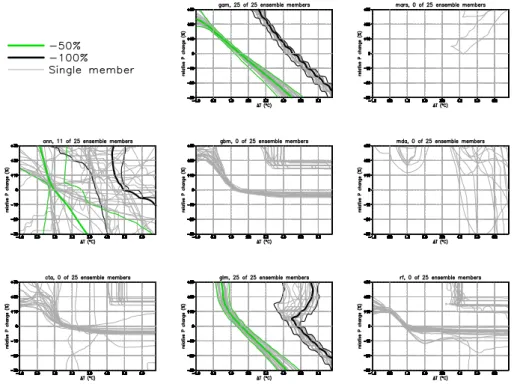
Impact response surfaces of the full ensemble of palsa climatic envelope models
Figures A1–A3 present impact response surfaces of all 600 palsa climatic envelope models.
Appendix B
Combination of parameter and initial conditions uncertainties
Fig. A1.Impact response surfaces showing the combinations of changes in annual mean temperature and precipitation for which half (green lines) and all (black lines) of the simulated palsa area becomes unsuitable relative to the simulated distribution for the 1961–1990 baseline period for eight climatic envelope modelling techniques. The thicker lines show values for ensemble averages of all plausible models (see text) calibrated for the 1951–1980 baseline period, the thinner lines show the range for the ensembles. Impact response surfaces of individual models, including those that failed the plausibility criteria, are shown with gray lines. The name of the technique and the number of plausible models is given as a title for each sub-graph.
Fig. A3.As in Fig. A1, but for models calibrated for the 1971–2000 baseline period.
Probab
il
ity
(%)
50
60
70
80
90
100
G
AM
51
80
G
AM
61
90
G
AM
71
00
50
60
70
80
90
100
Si
m
p
le
50
60
70
80
90
100
A
dj
us
ted
m
e
an
50
60
70
80
90
100
50
60
70
80
90
100
Fig. A4. Confidence intervals on probabilities of all palsa areas
becoming unsuitable by 2080–2099 estimated with GAM ensem-bles calibrated for different baseline periods (1951–1980, 1961– 1990, 1971–2000; gray boxplots), two approaches for estimating the combined parameter and initial conditions uncertainty by a sim-ple sum of the individual distributions (darkgray boxplots) and by summing re-sampled distributions with adjusted mean (orange box-plots). Probabilities were estimated by evaluating the impact re-sponse surface for the Grand Ensemble (n= 10 000) with SRES
A1B forcing. Boxplots show lower quartile, median and upper quartile; triangle peaks show the 5th and 95th percentiles (defin-ing 90 % confidence intervals); whiskers delimit the smallest and largest values.
(GAM5180, GAM6190 and GAM7100 in Fig. A4), but has thinner tails then a simple combination of these three distri-butions (labelled “Simple” in Fig. A4).
Acknowledgements. We thank Glen Harris, Met Office Hadley Centre, for providing probabilistic climate change projections and Ines H¨oschel, Freie Universit¨at Berlin, for regional averages of AOGCM simulations. We thank Risto K. Heikkinen for fruitful discussions and Pam Berry, Jørgen Olesen and one anonymous referee for providing constructive comments on an earlier version of this manuscript. This study was funded by the European Com-mission’s Sixth Framework Programme through the ENSEMBLES project (contract GOCE-CT-2003-505539) and by the Academy of Finland (decisions 127239 and 140806).
Edited by: J. E. Olesen
Reviewed by: M. Semenov and P. Berry
References
Ara´ujo, M. B. and New, M.: Ensemble forecasting of species distri-butions, Trends Ecol. Evol, 22, 42–47, 2007.
Ara´ujo, M. B., Pearson, R. G., Thuiller, W., and Erhard, M.: Val-idation of species-climate impact models under climate change, Global Change Biol., 11, 1504–1513, 2005.
D´equ´e, M. and Somot, S.: Weighted frequency distributions express modelling uncertainties in the ENSEMBLES regional climate experiments, Clima. Res., 44, 195–209, doi:10.3354/cr00866, 2010.
Elith, J., Leathwick, J. R., and Hastie, T.: A working guide to boosted regression trees, J. Anim. Ecol., 77, 802–813, doi:10.1111/j.1365-2656.2008.01390.x, 2008.
Fronzek, S. and Carter, T. R.: Assessing uncertainties in climate change impacts on resource potential for Europe based on pro-jections from RCMs and GCMs, Climatic Change, 81 (Suppl. 1), 357–371, 2007.
Fronzek, S., Luoto, M., and Carter, T. R.: Potential effect of climate change on the distribution of palsa mires in subarctic Fennoscan-dia, Clima. Res., 32, 1–12, 2006.
Fronzek, S., Carter, T. R., R¨ais¨anen, J., Ruokolainen, L., and Luoto, M.: Applying probabilistic projections of cli-mate change with impact models: a case study for sub-arctic palsa mires in Fennoscandia, Climatic Change, 99, 515–534, doi:10.1007/s10584-009-9679-y, 2010.
Harris, G. R., Collins, M., Sexton, D. M. H., Murphy, J. M., and Booth, B. B. B.: Probabilistic projections for 21st century Eu-ropean climate, Nat. Hazards Earth Syst. Sci., 10, 2009–2020, doi:10.5194/nhess-10-2009-2010, 2010.
Heikkinen, R. K., Luoto, M., Ara´ujo, M. B., Virkkala, R., Thuiller, W., and Sykes, M. T.: Methods and uncertainties in bioclimatic envelope modelling under climate change, Prog. Phys. Geog., 30, 751–777, 2006.
Heikkinen, R. K., Luoto, M., Kuussaari, M., and Toivonen, T.: Modelling the spatial distribution of a threatened butterfly: Im-pacts of scale and statistical technique, Landscape and Urban Plann., 79, 347–357, 2007.
Jeschke, J. M. and Strayer, D. L.: Usefulness of Bioclimatic Models for Studying Climate Change and Invasive Species, Ann. NY. Acad. Sci., 1134, 1–24, doi:10.1196/annals.1439.002, 2008. Johns, T., Royer, J. F., H¨oschel, I., Huebener, H., Roeckner, E.,
Manzini, E., May, W., Dufresne, J. L., Otter˚a, O., van Vu-uren, D., Salas y Melia, D., Giorgetta, M., Denvil, S., Yang, S., Fogli, P., K¨orper, J., Tjiputra, J., Stehfest, E., and Hewitt, C.: Climate change under aggressive mitigation: the ENSEMBLES multi-model experiment, Clim. Dynam., doi:10.1007/s00382-011-1005-5, 2011.
Jones, R. N.: Managing Uncertainty in Climate Change Projections – Issues for Impact Assessment, Climatic Change, 45, 403–419, 2000a.
Jones, R. N.: Analysing the risk of climate change using an irriga-tion demand model, Clima. Res., 14, 89–100, 2000b.
Kauppi, P. and Posch, M.: Sensitivity of boreal forests to possible climatic warming, Climatic Change, 7, 45–54, 1985.
Landis, J. R. and Koch, G. G.: The Measurement of Observer Agreement for Categorical Data, Biometrics, 33, 159–174, 1977. Lowe, J. A., Hewitt, C. D., van Vuuren, D. P., Johns, T. C., Stehfest, E., Royer, J.-F., and van der Linden, P. J.: New Study For Climate Modeling, Analyses and Scenarios, Eos, Trans. Am. Geophys. Union, 90, 181, doi:10.1029/2009EO210001, 2009.
Luo, Q., Bellotti, W., Williams, M., Cooper, I., and Bryan, B.: Risk analysis of possible impacts of climate change on South Aus-tralian wheat production, Climatic Change, 85, 89–101, 2007. Luoto, M. and Sepp¨al¨a, M.: Thermokarst ponds as indicators of
the former distribution of palsas in Finnish Lapland, Permafrost
Periglac., 14, 19–27, doi:10.1002/ppp.441, 2003.
Luoto, M., Fronzek, S., and Zuidhoff, F. S.: Spatial modelling of palsa mires in relation to climate in Northern Europe, Earth Surf. Proc. Land., 29, 1373–1387, 2004a.
Luoto, M., Heikkinen, R. K., and Carter, T. R.: Loss of palsa mires in Europe and biological consequences, Environ. Conserv., 31, 1–8, 2004b.
Luoto, M., Marmion, M., and Hjort, J.: Assessing spa-tial uncertainty in predictive geomorphological mapping: A multi-modelling approach, Comput. Geosci., 36, 355–361, doi:10.1016/j.cageo.2009.07.008, 2010.
Marmion, M., Hjort, J., Thuiller, W., and Luoto, M.: A comparison of predictive methods in modelling the distribution of periglacial landforms in Finnish Lapland, Earth Surf. Proc. Land., 33, 2241– 2254, doi:10.1002/esp.1695, 2008.
Marmion, M., Luoto, M., Heikkinen, R. K., and Thuiller, W.: The performance of state-of-the-art modelling techniques depends on geographical distribution of species, Ecol. Model., 220, 3512– 3520, 2009.
Mitchell, T. D., Carter, T. R., Jones, P. D., Hulme, M., and New, M.: A comprehensive set of high-resolution grids of monthly climate for Europe and the globe: the observed record (1901–2000) and 16 scenarios (2001–2100), Tyndall Centre Working Paper, 55, 29 pp., 2004.
Murphy, J. M., Booth, B. B. B., Collins, M., Harris, G. R., Sex-ton, D. M. H., and Webb, M. J.: A methodology for probabilistic predictions of regional climate change from perturbed physics ensembles, Philosophical Transactions of the Royal Society A, Mathematical Physical and Engineering Sciences, 365, 1993– 2028, doi:10.1098/rsta.2007.2077, 2007.
Naki´cenovi´c, N., Alcamo, J., Davis, G., de Fries, B., Fenhann, J., Gaffin, S., Gregory, K., Gr¨ubler, A., Jung, T. Y., Kram, T., La Rovere, E. L., Michaelis, L., Mori, S., Morita, T., Pepper, W., Pitcher, H., Price, L., Raihi, K., Roehrl, A., Rogner, H.-H., Sankovski, A., Schlesinger, M., Shukla, P., Smith, S., Swart, R., von Rooijen, S., Victor, N., and Dadi, Z.: Emissions Scenarios, A Special Report of Working Group III of the Intergovernmental Panel on Climate Change, Cambridge University Press, Cam-bridge, 599, 2000.
New, M., Lister, D., Hulme, M., and Makin, I.: A high-resolution data set of surface climate over global land areas, Clima. Res., 21, 1–25, 2002.
New, M., Lopez, A., Dessai, S., and Wilby, R.: Challenges in using probabilistic climate change information for impact assessments: an example from the water sector, Philos. T. Roy. Soc. A, 365, 2117–2131, 2007.
R¨ais¨anen, J. and Ruokolainen, L.: Probabilistic forecasts of near-term climate change based on a resampling ensemble technique, Tellus, 58, 461–472, 2006.
R¨otter, R. P., Carter, T. R., Olesen, J. E., and Porter, J. R.: Crop-climate models need an overhaul, Nat. Clim. Change, 1, 175– 177, doi:10.1038/nclimatE1152, 2011.
Roubicek, A. J., VanDerWal, J., Beaumont, L. J., Pitman, A. J., Wilson, P., and Hughes, L.: Does the choice of climate baseline matter in ecological niche modelling?, Ecol. Model., 221, 2280– 2286, 2010.
Sepp¨al¨a, M.: Synthesis of studies of palsa formation underlining the importance of local environmental and physical characteristics, Quaternary Res., 75, 366–370, 2011.
Swets, K.: Measuring the accuracy of diagnostic systems, Science, 240, 1285–1293, 1988.
Thuiller, W.: BIOMOD – optimizing predictions of species dis-tributions and projecting potential future shifts under global change, Global Change Biol., 9, 1353–1362, doi:10.1046/j.1365-2486.2003.00666.x, 2003.
Thuiller, W., Lafourcade, B., Engler, R., and Ara´ujo, M. B.: BIOMOD – a platform for ensemble forecasting of species distributions, Ecography, 32, 369–373, doi:10.1111/j.1600-0587.2008.05742.x, 2009.
van der Linden, P. and Mitchell, J. F. B.: ENSEMBLES: Climate Change and its Impacts: Summary of research and results from the ENSEMBLES project, Met Office Hadley Centre, FitzRoy Road, Exeter EX1 3 PB, UK, 160, 2009.
van Vuuren, D., den Elzen, M., Lucas, P., Eickhout, B., Strengers, B., van Ruijven, B., Wonink, S., and van Houdt, R.: Stabilizing greenhouse gas concentrations at low levels: an assessment of reduction strategies and costs, Climatic Change, 81, 119–159, doi:10.1007/s10584-006-9172-9, 2007.