www.clim-past.net/7/1041/2011/ doi:10.5194/cp-7-1041-2011
© Author(s) 2011. CC Attribution 3.0 License.
of the Past
Sensitivity of interglacial Greenland temperature and
δ
18
O:
ice core data, orbital and increased CO
2
climate simulations
V. Masson-Delmotte1, P. Braconnot1, G. Hoffmann1, J. Jouzel1, M. Kageyama1, A. Landais1, Q. Lejeune1, C. Risi2, L. Sime3, J. Sjolte4, D. Swingedouw1, and B. Vinther4
1Laboratoire des Sciences du Climat et de l’Environnement, UMR8212, CEA-CNRS-UVS, Gif-sur-Yvette, France 2CIRES, U. Colorado, Boulder, USA
3British Antarctic Survey, Cambridge, UK
4Centre for Ice and Climate, Niels Bohr Institute, University of Copenhagen, Copenhagen, Denmark Received: 17 May 2011 – Published in Clim. Past Discuss.: 23 May 2011
Revised: 2 September 2011 – Accepted: 2 September 2011 – Published: 29 September 2011
Abstract. The sensitivity of interglacial Greenland tem-perature to orbital and CO2 forcing is investigated using the NorthGRIP ice core data and coupled ocean-atmosphere IPSL-CM4 model simulations. These simulations were con-ducted in response to different interglacial orbital configu-rations, and to increased CO2concentrations. These differ-ent forcings cause very distinct simulated seasonal and lat-itudinal temperature and water cycle changes, limiting the analogies between the last interglacial and future climate. However, the IPSL-CM4 model shows similar magnitudes of Arctic summer warming and climate feedbacks in response to 2×CO2and orbital forcing of the last interglacial period (126 000 years ago).
The IPSL-CM4 model produces a remarkably linear re-lationship between TOA incoming summer solar radiation and simulated changes in summer and annual mean central Greenland temperature. This contrasts with the stable iso-tope record from the Greenland ice cores, showing a multi-millennial lagged response to summer insolation. During the early part of interglacials, the observed lags may be ex-plained by ice sheet-ocean feedbacks linked with changes in ice sheet elevation and the impact of meltwater on ocean cir-culation, as investigated with sensitivity studies.
A quantitative comparison between ice core data and cli-mate simulations requires stability of the stable isotope – temperature relationship to be explored. Atmospheric sim-ulations including water stable isotopes have been conducted with the LMDZiso model under different boundary condi-tions. This set of simulations allows calculation of a temporal
Correspondence to: V. Masson-Delmotte ([email protected])
Greenland isotope-temperature slope (0.3–0.4 ‰ per ◦C) during warmer-than-present Arctic climates, in response to increased CO2, increased ocean temperature and orbital forc-ing. This temporal slope appears half as large as the modern spatial gradient and is consistent with other ice core esti-mates. It may, however, be model-dependent, as indicated by preliminary comparison with other models. This sug-gests that further simulations and detailed inter-model com-parisons are also likely to be of benefit.
Comparisons with Greenland ice core stable isotope data reveals that IPSL-CM4/LMDZiso simulations strongly un-derestimate the amplitude of the ice core signal during the last interglacial, which could reach +8–10◦C at
fixed-elevation. While the model-data mismatch may result from missing positive feedbacks (e.g. vegetation), it could also be explained by a reduced elevation of the central Greenland ice sheet surface by 300–400 m.
1 Introduction
In principle, these data can provide a benchmark to test the ability of climate models to correctly represent climate feed-backs (Otto-Bliesner et al., 2006). Past changes in orbital forcing indeed provide natural externally forced experiments on the Earth’s climate, leading to past interglacial periods with Arctic temperatures warmer than present-day and large changes in Greenland ice sheet volume (Kopp et al., 2009; Vinther et al., 2009). In particular, the last interglacial pe-riod, about 130–120 thousand years before present (ka), is proposed to be a good analogue for future climate change driven by anthropogenic greenhouse gas emissions (Clark and Huybers, 2009; Otto-Bliesner et al., 2006; Sime et al., 2009; Turney and Jones, 2010), especially in the Arctic.
In this manuscript, we address the following questions: – What is the Greenland ice core quantitative information
on past surface temperature changes during the current and last interglacial, and how is it related to orbital forc-ing? This requires the relationship between Greenland surface temperature and snowfall isotopic composition, and the various processes that can modify this relation-ship through time, to be understood.
– Which changes in Greenland climate are produced by an ocean-atmosphere model in response to different in-terglacial orbital configurations? For this purpose, we analyze long snapshot simulations conducted with the IPSL-CM4 model forced only by the orbital configura-tion of key periods of the current and last interglacial at 0, 6, 9.5, 115 and 126 ka. For 126 ka, we also consider a sensitivity test to a simple parameterization of Green-land ice sheet melt allowing representation of the impact of meltwater on the ocean circulation (Swingedouw et al., 2009).
– What are the analogies and differences between the cli-mate response to the forcings associated with increased CO2 concentrations and to changes in orbital configu-ration? For this purpose, we compare the IPSL-CM4 response to higher atmospheric CO2concentrations and to the last interglacial insolation change, with a focus on Greenland climate. Indeed, climate projections (2× and 4×CO2) give access to climate states with 3 to 8◦C warmer central Greenland annual mean
tempera-ture (Masson-Delmotte et al., 2006b).
– Is the climate model able to capture the magnitude of changes derived from the ice core data? For direct model-data comparisons, we use the sea surface con-ditions (sea surface temperature, SST and sea ice) from the coupled climate model to drive its atmospheric com-ponent equipped with the explicit modeling of precipita-tion isotopic composiprecipita-tion (LMDZiso). This also allows the stability of the isotope-temperature change through time and the mechanisms that can alter this relationship to be explored.
– What was the change in central Greenland ice sheet to-pography during the last interglacial? The IPSL-CM4 and LMDZiso simulations appear to underestimate the magnitude of last interglacial temperature and precip-itation isotopic composition changes compared to the Greenland ice core data. Assuming that the model-data mismatch is mainly caused by a reduced ice sheet ele-vation, we can estimate the magnitude of this elevation change.
In order to address these questions, Sect. 2 is dedicated to the information obtained from the NorthGRIP ice core. Sec-tion 3 describes the results of the IPSL-CM4 coupled ocean-atmosphere model climate under different orbital configu-rations. The response of the central Greenland climate to orbital forcing is also compared to its response to projec-tions of higher greenhouse gas concentraprojec-tions. An analysis of the key radiative feedbacks affecting the top of the atmo-sphere radiative budget is proposed. In Sect. 4, we investigate the Greenland isotope-temperature relationship for warmer-than-present climates using isotopic atmospheric general cir-culation models (LMDZiso and HadAM3iso) and discuss the implications for past central Greenland temperature and pos-sible elevation changes.
2 Ice core information on past Greenland temperature
2.1 Water stable isotopes – climate relationships
Continuous records of water stable isotopes (δ18O or δD) have been measured along several deep Greenland ice cores; the longest record published so far was obtained from the NorthGRIP ice core (NorthGRIP-community-members, 2004) (Fig. 1). The initial vapour is formed by evaporation at the ocean surface. Its isotopic composition is affected by evaporation conditions through equilibrium and kinetic frac-tionation processes, and it depends on moisture sources tem-perature and relative humidity. Along the air mass trajec-tories to Greenland, the isotopic composition of the atmo-spheric water vapour undergoes mixing by convection, up-load of new water vapor from different sources, and distilla-tion linked with the progressive air mass cooling and succes-sive condensation, as well as kinetic effects on ice crystals. Altogether, these physical processes result in a linear rela-tionship between the air temperature and the snowfall iso-topic composition in central Greenland. Forδ18O, the slope of the modern spatial relationship is 0.7 ‰ per◦C for the first
ice core sites (e.g. Dye 3, Camp Century) (Dansgaard, 1964), and 0.8 ‰ per◦C for all available data including coastal
sta-tions (Dansgaard, 1964; Sjolte et al, 2011).
In addition to the impact of condensation temperature, sev-eral effects can affect the precipitation isotopic composition and modify the temporal isotope-temperature relationship
– deposition effects, caused by precipitation intermittency
-44 -42 -40 -38 -36 -34 -32 -30
NGRIP
δ
18 O ( o /oo
)
140 120 100 80 60 40 20 0
Age (ky)
-25 -20 -15 -10 -5
0
NGRIP
Δ
T (°C)
40x10-3 20 0 -20 -40
Precession
0.42
0.41
0.40
0.39
Obliquity
40x10-3
30
20
10
Eccentricity
280
260
240
220
200
CO
2
(ppmv)
-80 -40 0 Sea level (m)
560
520
480
75°N June (W/m²)
0 6 9.5 115
122 126
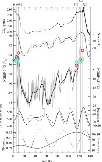
Fig. 1.From top to bottom: black dots, atmospheric CO2
concen-tration (Vostok and EDC ice cores) on the EDC3 age scale (Barnola et al., 1987; Lourantou et al., 2010); solid black line with uncer-tainties, estimation of eustatic sea level (Waelbroeck et al., 2002);
NorthGRIP ice coreδ18O data on a 20 year resolution on GICC05
and EDC3 age scale (Capron et al., 2010a). The orbital component of the record is displayed (thick black line) and was calculated using the first three components of a singular spectrum analysis. A tenta-tive estimate of the temperature change is also displayed, following Masson-Delmotte et al. (2005b) (right axis). The reconstruction of the Holocene Greenland temperature (at fixed elevation) (Vinther et al., 2009) is displayed as a bold blue line. Summer (red) and annual mean (green) temperature anomalies simulated by the IPSL model are displayed as open circles for 6, 9.5, 115, 122, and 126 ka. The
75◦N June insolation (black line, W m−2) and orbital parameters
(precession parameter – long dashed line, obliquity – short dashed line, and eccentricity – solid black line) are displayed in the two lowest panels.
at the condensation level and the surface tempera-ture (Jouzel et al., 1997). Modern observations sug-gest greater summer than winter precipitation in cen-tral Greenland (Shuman et al., 1995), which differs from deposition seasonality in Antarctica (Laepple et
al., 2011). Atmospheric models have shown a large deposition effect for Greenland glacial climate, due to strongly reduced winter precipitation (Krinner et al., 1997; Werner et al., 2000). In this manuscript, we assess the “precipitation-weighting effect” by compar-ing the average temperature change to the monthly precipitation-weighted temperature change;
– source effects, caused by changes in evaporation
condi-tions or moisture origin (Johnsen et al., 1989; Jouzel et al., 2007; Masson-Delmotte et al., 2005a,c);
– glaciological effects, caused by changes in ice sheet
topography which affects surface air temperature and stable isotopic composition (Vinther et al., 2009). We therefore introduce the notion of temperature estimate “at fixed elevation”, by contrast with the information on air temperature at the ice sheet surface classically de-rived from stable isotope data (Masson-Delmotte et al., 2005a).
Alternative information on past Greenland temperature is available from the borehole temperature profiles (Dahl-Jensen et al., 1998) and from firn gas fractionation dur-ing abrupt warmdur-ings (Capron et al., 2010a; Severdur-inghaus et al., 1998). The latter method allows the estimation of the interstadial isotope-temperature slope to range between 0.30±0.05 and 0.60±0.05 ‰ ofδ18O per◦C (Capron et al., 2010a), therefore quite different from the spatial slope. This likely results from deposition and source effects (Masson-Delmotte et al., 2005a). In Sect. 4, we will use isotopic sim-ulations to quantify the isotope-temperature relationship in warmer-than-present climate conditions.
2.2 Greenland Holocene climate and ice sheet elevation
Recently, Vinther et al. (2009) conducted a synthesis of the Greenland ice core Holocene stable isotope information. It combines ice core records from coastal ice caps (where changes in elevation are limited) and from the central ice sheet (where higher elevation changes can significantly af-fect the isotopic signals). The authors extract a common and homogeneous annual mean Greenland temperature signal “at fixed elevation”, together with regional changes in the ice sheet topography. The new “fixed elevation” temperature his-tory from this study (Fig. 1, central panel, blue line) reveals a pronounced Holocene climatic optimum in Greenland coin-ciding with a maximum thinning near the ice sheet margins. These results also imply that the NorthGRIP ice coreδ18O data can be converted to temperature with a temporal slope of 0.45 ‰ per◦C.
This plateau occurs 1.8 to 4.3 kyr (thousand years) later than the maximum in 75◦N June insolation. The early Holocene
warmth is partly masked in the central Greenland ice core stable isotope records because of the larger volume and ele-vation of the ice sheet.
2.3 Links between NorthGRIPδ18O and 75◦N summer insolation
We extract the orbital components of the NorthGRIP record using the first components of a Singular Spectrum Analy-sis performed on the whole series and corresponding to pe-riodicities longer than 3 kyr (Fig. 1, bold line, central panel). With the available ice core age scales (Capron et al., 2010b; Svensson et al., 2008), the orbital component of the North-GRIPδ18O appears to lag the reversed precession parame-ter (in phase with local June insolation) by several millen-nia (Fig. 1). A significant correlation (R2= 0.27) is obtained between the smoothed NorthGRIP δ18O and 4 kyr earlier 75◦N June insolation. The four most recent optima in this
smoothed NorthGRIPδ18O record lag maxima in 75◦N June
insolation by 4.8, 4.8, 3.1 and 3.5 kyr, respectively (Fig. 1, dashed vertical lines). These lags are significantly larger than the GICC05 (Rasmussen et al., 2006; Svensson et al., 2008)) age scale uncertainty (∼80 years at 10 ka,∼440 years at 20 ka,∼1000 years at 30 ka and∼2600 years at 60 ka) and occur both under glacial and interglacial contexts.
For the Holocene, it is obvious that the Greenland op-timum (at ∼7–10 ka) occurs later than the 11 ka preces-sion minimum (local June insolation maximum), likely be-cause of the negative feedback linked with the Laurentide ice sheet albedo and weaker northward advection of heat in the Atlantic Ocean caused by the meltwater from deglaciat-ing Northern Hemisphere ice sheets (Renssen et al., 2009). The NorthGRIP record does not allow this aspect to be explored for the last interglacial because it does not span the whole length of this period (NorthGRIP-community-members, 2004). Marine sediment records of North At-lantic sea surface temperature suggest a pattern similar to the Holocene with a lag between peak insolation and peak iso-topic values (Masson-Delmotte et al., 2010a). During the end of the interglacials (after optima in insolation and in
δ18O), parallel decreasing trends in 75◦N June insolation and
NorthGRIPδ18O are observed. For the mid to late Holocene (the last 8 kyr), the δ18O-insolation slope is 0.02 ‰ per W m−2 (0.03 to 0.06◦C per W m−2), much weaker than for the end of the last interglacial (121 to 115 ka), where it reaches 0.10 ‰ per W m−2(∼0.17 to 0.33◦C per W m−2). 2.4 Last interglacial Greenland climate
The ice core information on central Greenland climate dur-ing the last interglacial is not as precise as for the Holocene due to the age scale uncertainty, the end of the NorthGRIP record at∼123 ka, and the lack of information from borehole
thermometry to constrain the isotope-temperature-elevation histories. Based on the shape of north Atlantic SST records synchronized on the EDC3 age scale (Masson-Delmotte et al., 2010a), one may assume that the isotopic values of the deepest part of the NorthGRIP ice core may be represen-tative of a multi-millennial temperature plateau. Consider-ing the uncertainty on the isotope-temperature relationship (between 0.3 and 0.8 ‰ per ◦C), the NorthGRIP Last In-terglacial ∼3 ‰ δ18O anomaly would translate into a 3.8– 10.0◦C surface temperature anomaly. The signal for the last interglacial is without doubt larger than for the early to mid Holocene (see Sect. 2.2), as expected from the larger orbital forcing (Fig. 1).
By themselves, the data do not allow us to quantify the deposition or glaciological effects affecting this temperature estimate, motivating the use of climate models to explore the mechanisms controlling precipitation isotopic composition.
3 Climate modelling
3.1 IPSL-CM4 coupled climate model simulations
The IPSL-CM4 coupled climate model has been extensively used for CMIP3 and PMIP2 simulations (Alkama et al., 2008; Born et al., 2010; Braconnot et al., 2007, 2008; Kageyama et al., 2009; Marti et al., 2010; Swingedouw et al., 2006). The model couples the atmospheric component LMDZ (Hourdin et al., 2006) with the OPA ocean compo-nent (Madec and Imbard, 1996). A sea ice model (Fichefet and Maqueda, 1997) which computes the ice thermodynam-ics and physthermodynam-ics is coupled with the ocean-atmosphere model. The ocean and atmosphere exchange momentum, heat and freshwater fluxes, as well as surface temperature and sea ice once a day, using the OASIS coupler (Valcke, 2006). None of the fluxes are corrected or adjusted. The model is run with a horizontal resolution of 96 points in longitude and 71 points in latitude (3.75◦×2.5◦) for the atmosphere and 182 points
in longitude and 149 points in latitude for the ocean. There are 19 vertical levels in the atmosphere and 31 levels in the ocean, where the highest resolution (10 m) is focused on the upper 150 m. The model reproduces the main features of modern climate, although large temperature or precipitation biases can be partly related to the resolution (Marti et al., 2010). The North Atlantic is often marked by large cold bi-ases in coupled climate models. This is also the case for IPSL-CM4 where a weak Atlantic Meridional Oceanic Cir-culation (AMOC) (Swingedouw et al., 2007) is linked with a cold bias for central Greenland.
et al., 2010b). These previous studies showed that the IPSL-CM4 model response is comparable to other climate models and generally seems to underestimate the magnitude of tem-perature changes compared to those derived from the ice core data.
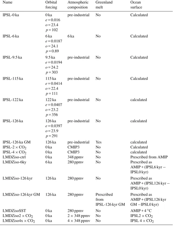
A set of simulations has been conducted to explore the re-sponse of the model to various orbital configurations encoun-tered during the current and last interglacial (see the grey ver-tical bars in Fig. 1 and the simulation descriptions in Table 1), with all other boundary conditions kept as for the model control simulation (pre-industrial). Small changes in atmo-spheric composition (CO2, CH4)leading to radiative pertur-bations<0.4 W m−2during the current and last interglacial were neglected, except for the 6 ka simulation following the PMIP2 protocol (Braconnot et al., 2007). The time periods for these simulations (at 0, 6, 9.5, 115, 122 and 126 ka) were chosen to represent contrasting changes in the seasonal cy-cle of insolation, with different combinations of precession (rather similar at 0 and 115 ka, 122 and 6 ka, 9.5 and 126 ka), obliquity (maximum at 9.5 and minimum at 115 ka) and ec-centricity (minimum at 0 ka and maximum at 115 ka) con-figurations (Braconnot et al., 2008). These simulations were integrated from 300 to 1000 years depending on the time pe-riod (Table 1). Since changes in Earth’s orbital parameters only marginally affect the global annual mean simulations, these simulations adjust very rapidly to the insolation forc-ing (50–100 years) from the same initial state. We consider here mean annual cycles computed from 150 to 400 years. Our analysis focuses on the most contrasting simulations, 126 ka and 115 ka. Note that the Antarctic ice core data de-pict atmospheric CO2levels close to the pre-industrial (273– 276 ppmv) during these two time periods (Masson-Delmotte et al., 2010a).
We have also used a similar approach to that of Sime et al. (2008) whilst exploring different forms of warmer Greenland climates. We have therefore also analyzed sim-ulations run under projected increased CO2concentrations. The 2×CO2 simulation has been integrated for 250 years. Beginning from a pre-industrial simulation, the atmospheric CO2concentration is increased by 1 % per year until it dou-bles within 70 years (from 280 to 560 ppmv). It is then kept constant for the remaining 180 years. The same pro-tocol is followed for the 4×CO2simulation (quadrupling of CO2 in 140 years and then kept constant for the remaining 110 years). We have used the model outputs averaged over the last 100 years of these simulations.
While the topography of the Greenland and Antarctic ice sheet is constant for all the simulations, a parameterization of Greenland melt has been implemented in order to explore the feedbacks between Greenland warming, Greenland melt-water flux and thermohaline circulation (Swingedouw et al., 2009) with implications for monsoon areas (Braconnot et al., 2008). A simulation including this parameterisation under 126 ka orbital forcing was integrated for 350 years. The ther-mohaline circulation is affected by an additional freshwater
flux and adjusts within 150 years to the forcing. After this adjustment, the deep ocean drift is limited.
3.2 Impact of orbital forcing on IPSL-CM4 simulated central Greenland climate
Figure 2 displays the model results for central Greenland us-ing the same definition as in Masson-Delmotte et al. (2006a), that is the temperature averaged at places where ice sheet el-evation is above 1.3 km. For each simulation, monthly mean values of central Greenland temperatures are displayed as a function of monthly mean values of 75◦N top of atmosphere (hereafter TOA) incoming solar radiation. The elliptic shape of the plots reflects the one month seasonal lag between sur-face air temperature and insolation, mostly because of the thermal inertia of the surrounding oceans affecting heat ad-vection to central Greenland. Orbital forcing alone has lim-ited impacts on the simulated winter temperature (because of a weak incoming insolation at that season and latitude) and a strong impact on summer-fall temperatures.
The simulated change in summer temperature is domi-nating the simulated annual mean temperature change (Ta-ble 2). Compared with the pre-industrial control simulation, July (respectively annual mean) temperature changes vary by −2.5◦C (−0.5◦C) for 115 ka to +5.8◦C (+0.9◦C) for 126 ka. The model results for summer and annual mean temperature are depicted in Fig. 1 with red and green open circles, respec-tively. This comparison suggests that the IPSL-CM4 simula-tion has the right sign of temperature changes, but underes-timates the magnitude of annual mean changes compared to the ice core derived information. We now explore the sim-ulated deposition effects, which can impact the model-data comparison, focusing on the precipitation weighting effect.
For all orbital contexts, the IPSL-CM4 model shows a positive precipitation weighting effect (difference be-tween monthly precipitation-weighted temperature and an-nual mean temperature) (Table 2, last column). This effect is minimum at 115 ka (1.8◦C), maximum at 126 ka (5.2◦C) and is strongly enhanced with increasing local summer inso-lation. This is due to a strong (non linear) enhancement of summer precipitation for warmer summer temperatures (Ta-ble 2). The IPSL-CM4 model therefore points to a large de-position effect, suggesting that the Greenland ice core warms interglacial proxy records such as stable isotopes, but also 10Be (Wagner et al., 2001; Yiou et al., 1997) may be biased towards summer. The simulated changes in precipitation-weighted temperature are intermediate between the summer and annual mean temperature and vary between−1.1◦C (at
115 ka) and +3.6◦C (at 126 ka) (Table 2).
Table 1. Description of the simulations. The LMDZiso simulations were run for 5 years with climatological forcing averaged from the IPSL-CM4 ouputs, and results analysed for the last 3 years of this simulation. AMIP (Atmospheric Modelling Intercomparison Project) boundary conditions are derived from observed SST and sea-ice (1979 to 2007). Atmospheric composition refers to prescribed changes in
greenhouse gas concentrations (e.g. CO2). In the orbital forcing column,e,oandprespectively stand for eccentricity, obliquity (in◦), and
perihelia-180◦.
Name Orbital Atmospheric Greenland Ocean
forcing composition melt surface
IPSL-0 ka 0 ka pre-industrial No Calculated
e= 0.016
o= 23.4
p= 102
IPSL-6 ka 6 ka 6 ka No Calculated
e= 0.0187
o= 24.1
p= 0.89
IPSL-9.5 ka 9.5 ka pre-industrial No Calculated
e= 0.0194
o= 24.2
p= 303
IPSL-115 ka 115 ka pre-industrial No Calculated
e= 0.0414
o= 22.4
p= 111
IPSL-122 ka 122 ka pre-industrial No calculated
e= 0.0407
o= 23.2
p= 356
IPSL-126 ka 126 ka pre-industrial No calculated
e= 0.0397
o= 23.9
p= 291
IPSL-126 ka GM 126 ka pre-industrial Yes calculated
IPSL-2×CO2 0 ka CMIP3 No Calculated
IPSL-4×CO2 0 ka CMIP3 No calculated
LMDZiso-ctrl 0 ka 348 ppmv No Prescribed from AMIP
LMDZiso-6ky 6 ka 280 ppmv No Prescribed as
AMIP + (IPSL6 kyr−
IPSL0 kyr)
LMDZiso-126 kyr 126 ka 280 ppmv No Prescribed as
AMIP + (IPSL126 kyr−
IPSL0 kyr)
LMDZiso-126 kyr GM 126 ka 280 ppmv Prescribed Prescribed as
from AMIP + (IPSL126 kyr
IPSL-126 kyr GM GM−IPSL0 kyr)
LMDZisoSST 0 ka 280 ppmv No AMIP + 4◦C
LMDZiso2×CO2 0 ka 2×348 ppmv No IPSL2×CO2
LMDZiso4x×CO2 0 ka 4×348 ppmv No IPSL 4×CO2
response to summer insolation therefore appears at least half as large as that derived from the ice core data for the tran-sition from 122 to 115 ka (0.17 to 0.33◦C per W m−2, see Sect. 2.3). In Sect. 3.2, we investigate the changes affecting
Table 2.IPSL-CM4 results for Greenland (from grid points located above 1300 m elevation): annual mean, July and precipitation-weighted
temperature (◦C) as well as deposition effect (difference between precipitation-weighted and annual mean temperature) and ratio of summer
(April–September) to annual precipitation. Results are given for the different simulations in response to orbital forcing only. Absolute values are given as well as anomalies with respect to the control simulation (numbers shown between parentheses).
Simulation Annual mean July Greenland Ratio of summer Precipitation Deposition
Greenland temperature half year (April– weighted effect
temperature (anomaly) (◦C) September) to Greenland (anomaly) (◦C)
(anomaly) (◦C) annual temperature
precipitation (anomaly)
(percentage of (◦C)
change)
Control simulation −28.3 −12.9 0.60 −25.9 2.4
6 ka −27.9 (+0.4) −10.6 (+2.3) 0.62 (+3 %) −24.7 (+1.2) 3.2 (+0.7)
9.5 ka −27.5 (+0.8) −8.5 (+4.4) 0.65 (+8 %) −23.3 (+2.6) 4.2 (+1.8)
115 ka −28.8 (−0.5) −15.4 (−2.5) 0.58 (−3 %) −27.0 (−1.1) 1.8 (−0.7)
122 ka −28.1 (+0.2) −11.9 (+1.0) 0.62 (+3 %) −25.1 (+0.8) 3.0 (+0.6)
126 ka −27.4 (+0.9) −7.1 (+5.8) 0.68 (+13 %) −22.3 (+3.6) 5.2 (+2.7)
-16 -14 -12 -10 -8 -6
Warmest month T (°C) 440 480 520 560 Maximum monthly insolation (W/m²)
-40 -35 -30 -25 -20 -15 -10 -5
Monthly temperature (°C)
600 500 400 300 200 100 0
Monthly insolation (W/m²)
y=0.08x-51.97 (R²=0.99) a)
b)
1 2 3
4
5 6 7
8
9
10
11 12
0 6 9.5 115 122 126
Fig. 2. (a)Seasonal cycle of IPSL model simulated central
Green-land (>1300 m) temperature (◦C) as a function of the seasonal
cy-cle of TOA incoming solar radiation at 75◦N (W m−2) for different
orbital configurations (0, 6, 9.5, 115, 122 and 126 ka). For each period, the monthly data are displayed; black numbers indicate the number of the month (from 1 for January to 12 for December). The elliptic shape results from the phase lag between temperature and
insolation. (b)Regression between maximum monthly insolation
and the IPSL model central Greenland maximum monthly summer temperature (occurring one month after maximum insolation). A
linear relationship is observed, with a slope of 0.08◦C per W m−2.
The same color code is used as in panel a for the various simula-tions.
When taking into account the ocean circulation changes linked with a parameterization of Greenland melt at 126 ka, the IPSL-CM4 model simulates a 0.6◦C weaker July (resp. 0.4◦C annual) warming than in the standard 126 ka simulation (not shown in Table 2). In this simulation, the
AMOC is weakened because deep water formation in the North Atlantic/Nordic Seas is reduced by the Greenland ice sheet meltwater. The meridional heat transport by the atmo-spheric circulation is enhanced to compensate for the reduc-tion in ocean heat transport but the Arctic cools because of a larger sea ice extent. Therefore, taking into account the im-pact of ice sheet melting on the ocean circulation increases the model-data mismatch.
3.3 Differences between increased CO2and orbitally forced IPSL-CM4 climate responses
The orbital forcing has a negligible impact as such on the global and annual radiative forcing (<0.3 W m−2 over the last 130 ka), which contrasts with the 3.7 W m−2 radiative forcing for 2×CO2 (resp. 7.4 W m−2 for 4×CO2). Note that obliquity affects the latitudinal distribution of annual in-solation, with opposite effects at low and high latitudes (not shown), and a range of variations of resp. 4.5 to 10.5 W m−2 at 75◦N along the current and last interglacial (0–12 ka and
115–130 ka).
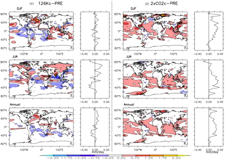
Moreover, the diurnal and seasonal distributions of orbital and 2×CO2forcings are drastically different. For 126 ka, anomalies (relative to pre-industrial) in summer insolation exceed 50 W m−2at mid and high northern latitudes (Fig. 3a, showing TOA radiative budget) at 126 ka, with large sea-sonal and latitudinal contrasts (Fig. 3b). This differs from the more homogeneous forcing caused by increased CO2 concentrations.
(b) 2xCO2c‐PRE (a) 126Kc‐PRE
Months Months
W/m2
°C °C
(d) (c)
Fig. 3. Comparison of anomalies between the last interglacial and pre-industrial control IPSL model simulations (left panel) and 2×CO2
and pre-industrial control simulation (right panel) for :(a)and(b)TOA net radiative budget (W m−2);(c)and(d)surface air temperature
(◦C) and(e)and(f)evaporation (mm day−1). For panels(a)and(b), anomalies are displayed as a function of month number (horizontal
axis) and latitude (vertical axis). For panels(c)to(f), anomalies are displayed as a function of longitude and latitude, for DJF
(December-January-February), JJA (June-July-August) and for the annual mean. On the right side of each panel(c)to(f), zonal mean anomalies are also
displayed as a function of latitude.
interglacial (126 ka) and pre-industrial for JJA, DJF and an-nual mean temperature, as well as their zonal mean, and compares them to the differences between 2×CO2 and present day for JJA, DJF and annual mean temperature. In-creased CO2 leads to simulated warming at low latitudes and a larger magnitude of warming at both poles (relative
mm/day mm/day
(e) (f)
Fig. 3.Continued.
insolation (Fig. 3a), with the exception of the Arctic, where a year round persistent warming is simulated. Such a feature is model-dependent, as shown by the comparison between the IPSL-CM4 results and other coupled model simulations for the seasonal cycle of simulated last interglacial temperature anomalies for Greenland (Masson-Delmotte et al., 2010c).
Figure 4 shows that the control simulation correctly cap-tures the amplitude and extrema of the observed Northern Hemisphere sea-ice cover (Rayner et al., 2003), but has a slight shift (one month earlier than in the data) in the sea-sonal cycle. In response to 126 ka orbital forcing, the model produces a summer sea ice retreat of∼3 million km2. This represents half of the retreat (∼6 million km2) simulated for 2x×CO2. In the 126 ka simulation, a small winter sea ice retreat is also simulated. This can be attributed to the large uptake of heat during summer in the high latitude ocean as well as to an enhanced AMOC, which brings warm surface waters to the high latitudes (Born et al., 2010). This winter sea-ice retreat is probably the cause for the warmer winter temperatures at 126 ka compared to the control simulation (Fig. 3c).
Winter Arctic warming is particularly large under 2×CO2 forcing, reaching ∼8◦C, compared to the ∼2◦C Arctic
warming for 126 ka conditions. While this comparison high-lights the differences between the two types of simulations, and therefore the limitations of analogies between the last in-terglacial and future climate change, we would like to stress that the simulated summer Arctic warming at 126 ka reaches a magnitude (∼4◦C) comparable to summer Arctic warming forced by 2×CO2(see also Fig. 5d).
Fig. 4. Monthly seasonal cycle of Northern Hemisphere sea ice
extent for present day (black), 126 ka (red) and 2×CO2(blue)
sim-ulated by IPSL-CM4. Present day (1900–2010) climatological data (Rayner et al., 2003) are also displayed (dashed grey).
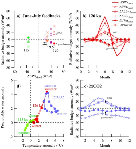
3.4 Analysis of radiative feedbacks
Following Braconnot et al. (2007), a simple feedback anal-ysis was performed in order to quantify the main drivers of changes in the top of the atmosphere radiative budget (TOA) at high latitudes (60–80◦N). The methodology for this
anal-ysis is described in Appendix A.
Figure 5 displays analyses of the TOA radiative budget terms and key feedbacks (represented by symbols) around Greenland. The different simulations are represented by the same colors as in Fig. 2. The specific radiative budgets for June–July are shown for all the orbitally forced simu-lations (Fig. 5a) and for each month for 126 ka (Fig. 5b) and 2×CO2 simulations (Fig. 5c). We do not display the changes in heat and water transport and only focus on the local radiation fluxes within the atmospheric column.
Figure 5a characterises the radiative feedbacks involved in the linear response of the IPSL-CM4 simulated summer Greenland surface temperature with respect to summer in-solation. At high northern latitudes, the different compo-nents of the radiative budget depict a linear relationship with respect to the change in incoming solar radiation at the top of the atmosphere1SWisimul. The net TOA shortwave flux (1SWnsimul, represented by “x”symbols) appears rel-atively close to the prescribed insolation change and only partially compensated for by increased longwave emission (1LWnsimul, represented by filled diamonds) so that the net radiative budget is positive (not shown).
At 6, 9.5, 122 and 126 ka, a strong positive shortwave feedback is linked with the total (surface and cloud) albedo effect (1ALBsimul, represented by “+” symbols). This fect is dominated by the clear sky (surface) albedo ef-fect (1ALB cssimul represented by the triangle symbols), only partly compensated by an enhanced negative cloud shortwave feedback (difference between1ALB cssimul and
1ALBsimul). The albedo feedback is consistent with changes in sea ice (Fig. 4). It increases almost linearly with the insola-tion forcing, stressing that the changes in clear sky shortwave surface radiation drive the surface radiative budget, surface temperature and thereby the snow and ice extent. Note that by construction, the total albedo feedback between the dif-ferent simulations lies on a line proportional to the planetary albedo of the control simulation. At 115 ka, clear sky and cloud albedo feedbacks have opposite signs and have a much smaller magnitude (with respect to the magnitude of the or-bital forcing) compared to other oror-bital simulations. The dif-ferent effects are thus not symmetrical for increased or re-duced insolation, certainly due to the temperature thresholds needed to build and melt snow and ice.
In addition, the longwave radiative budget changes (1LWnsimul, filled diamonds) appear to be driven by the changes in Planck emission directly caused by changes in surface temperature (1Plsimul, open diamonds). There is only a small increase in the atmospheric greenhouse effect caused by changes in the vertical temperature profile, wa-ter vapour content, and infra-red cloud radiative feedbacks (difference between the filled and open diamond symbols). This greenhouse feedback is too small to drive a non-linear response of the radiative budget around Greenland.
While this approach ignores the dynamical heat advection effects, it suggests that the top of the atmosphere radiative budget at high northern latitude is relatively linear with re-spect to orbital forcing and highlights the importance of the positive feedbacks linked with the surface albedo. The mag-nitude of the atmospheric greenhouse effect and the short-wave cloud negative feedback increase with the magnitude of the insolation forcing. In this model, the cloud feedback is enhanced for a warmer Arctic. Compensations of non-linearities of the Planck, albedo and cloud radiative effects at 115 ka likely explain the overall linearity of the IPSL-CM4 model high northern latitude temperature response to sum-mer insolation forcing.
6
4
2
0
-2
Precipitable water anomaly
8 6 4 2 0 -2 -4
Temperature anomaly (°C)
-80 -60 -40 -20 0 20 40 60 80
Radiative budget anomaly (W/m²)
12 10 8 6 4 2 0
Month
-80 -60 -40 -20 0 20 40 60 80
Radiative budget anomaly (W/m²)
12 10 8 6 4 2
Month -80
-60 -40 -20 0 20 40 60 80
Radiative budget anomaly (W/m²)
-80 -40 0 40 80
ΔSWisimul (W/m²)
d) c) 2xCO2
b) 126 ka a) June-July feedbacks
115
12269.5 126
2xCO2
126 ka
115 ka
cloud
greenhouse
summer
greenhouse cloud
cloud
greenhouse
summer
winter
winter
summer winter
ΔSWisimul
ΔSWnsimul
ΔALB cssimul
ΔALB simul
ΔLWnsimul ΔPlsimul
Fig. 5. Analysis of atmospheric feedbacks affecting the TOA radiative budget. (a)June–July changes in radiative budget terms (see text
and figure legend for details) as a function of June-July incoming solar radiation (W m−2), for different orbital contexts (6 ka, orange;
9.5 ka, violet; 115 ka, green; 122 ka, pink; and 126 ka, red). Arrows depict the magnitude of albedo (difference between “+” and triangle
symbols), cloud (difference between “+” and “x” symbols) and greenhouse (difference between open and filled diamonds) feedbacks for
126 ka. (b)Monthly values of the radiative budget 126 ka anomalies with respect to the control simulation (see text and legend for details)
(W m−2).(c)Same as(b)but for 2×CO2.(d)Seasonal cycle of precipitable water anomaly as a function of temperature anomaly (◦C) with
respect to the control simulation, for 115 ka (green), 126 ka (red) and 2×CO2(blue).
larger greenhouse feedbacks for 2×CO2in winter, as well as an earlier albedo feedback for 2×CO2, likely caused by the strongly reduced winter sea-ice cover in this simulation than for 126 ka (Fig. 4).
In order to better characterize the links between changes in surface temperature and atmospheric water content, Fig. 5d compares the seasonal cycle of atmospheric precipitable wa-ter anomaly as a function of surface temperature anomaly for 115, 126 ka and 2×CO2 simulations. The asymmetry between atmospheric moisture changes at 115 and 126 ka is obvious. Despite a completely different seasonality of the changes (with the 2×CO2 simulations showing its largest temperature changes in winter), the 126 ka and 2×CO2 sim-ulations again depict similar magnitudes of temperature and precipitable water changes, in summer.
4 Atmospheric modeling of water stable isotopes
4.1 Set up of the LMDZiso simulations
While water stable isotopes are not yet available in the cou-pled IPSL-CM4 model, they have been implemented in its at-mospheric component, LMDZ4 (Risi et al., 2010b) (hereafter called LMDZiso), with a standard resolution of 2.5◦×3.75◦.
and enriched bias at coastal stations. Comparable biases are found by other atmospheric models that include water stable isotopes (e.g. ECHAM and REMO-iso) (Sjolte et al., 2011). A suite of simulations has been conducted with the LMDZiso model, forced by the sea surface conditions and associated external forcings (6 ka and 126 ka orbital parame-ters, and increased greenhouse gas concentrations) simulated by the IPSL-CM4 model; a sensitivity test with 4◦C homo-geneous artificial increase in sea surface temperature com-pared to present-day (AMIP) has also been performed (Ta-ble 1). The isotopic simulations were run for 5 years, which is sufficient for the equilibration between the atmosphere and land surface reservoirs. We verified that trends in tempera-ture and stable isotopes over Greenland over the first 3 years of the simulations are lower than the standard deviations of the last 3 years, which were used for this study. We also ver-ified, using a longer 126 ka simulation (16 years), that the standard deviations calculated over a period of 3 years were not decreasing with a longer spin up period.
4.2 LMDZiso isotope-temperature relationships
Consistent with the coupled IPSL-CM4 simulations dis-cussed in Sect. 3, annual mean temperature changes simu-lated in central Greenland remain very small for the sim-ulations corresponding to changes in orbital configurations (<1◦C) (Fig. 6). They reach 4◦C for 2×CO
2, 6◦C for SST + 4◦C and ∼9◦C for 4×CO
2 simulations (Fig. 7). Deposition effects can be considered both for temperature and δ18O by calculating either annual mean or precipita-tion weighted values (Fig. 7). As discussed previously, this effect is particularly large for the orbitally forced simula-tions (up to 2◦C and 1 ‰, reaching magnitudes
compara-ble to the climate change signal). Because the CO2forcing increases both winter and summer temperature and precip-itation (Fig. 6), the resulting precipprecip-itation weighting effect is smaller (typically 1◦C and 0.5 ‰ for 4×CO2). This ef-fect enhances the magnitude of precipitation weightedδ18O anomalies (Fig. 7) and therefore slightly increases the “warm climate” isotope-temperature slope (from 0.30 to 0.36 ‰ per
◦C). Within all the studied simulations, the strength of the
correlation is comparable between annual mean precipita-tion isotopic composiprecipita-tion and temperature, and precipitaprecipita-tion weighted isotopic composition and temperature (R2>0.95,
n= 6) and larger than the correlation between precipita-tion weighted isotopic signal and annual mean temperature (R2= 0.86,n= 6). This suggests that the ice core data (cap-turing precipitation weighted information) should best be interpreted in terms of changes in precipitation-weighted temperature.
When considering all the available simulations, a lin-ear regression leads to a mean “warm climate” isotope-temperature slope of 0.31 ‰ per ◦C, with values ranging from 0.26 to 0.39 ‰ per◦C. This uncertainty is estimated by using either annual mean or precipitation weighting for
-35 -30 -25 -20 -15 -10 -5
0
Temperature (°C)
24 22 20 18 16 14 12 10 8 6 4 2 0
Month
14x10-6
12
10
8
6
4
2
Precipitation
-38 -36 -34 -32 -30 -28 -26 -24 -22
δ
18 Ο ( ο /οο
)
Control 6ka 126 ka 126 ka THC
2xCO2
4xCO2
SST+4
Fig. 6. Monthly seasonal cycle of temperature, precipitation and
precipitation δ18O simulated by LMDZiso for different sets of
boundary conditions (AMIP control, 6 ka, 126 ka, +4◦C SST, 2×
and 4x×CO2concentrations) prescribed using the IPSL-CM4 sea
surface conditions (see Table 1). For readability, the seasonal cycle has been repeated over 2 years (24 months).
temperature andδ18O, and by selections of 5 of the 6 sim-ulations to assess the uncertainty on each slope, which is about 0.03 ‰ per◦C. This simulated slope is consistent with
the lowest values derived from interstadial warming events (Capron et al., 2010a), with the slopes obtained using the borehole information at the glacial-interglacial scale (Cuffey and Clow, 1997; Dahl-Jensen et al., 1998), and lower than the slopes estimated during the current interglacial period after accounting for elevation changes (Vinther et al., 2009). This finding is also consistent with a small isotope-temperature slope simulated by the GISS model for the Holocene for Greenland (Legrande and Schmidt, 2009).
y = 0.36x R² = 0.83
y = 0.31x R² = 0.95
3
4
Last interglacial, ice core anomaly
4xCO2
y = 0.29x R² = 0.96
1
2
3
m
aly (‰)
126 ka SST+4°C6 ka
elevation ?
0
1
δ
18
O ano
m
mean T, weighted O
2xCO2
126 ka flux
6 ka
-2
-1
-2
0
2
4
6
8
10
mean T, mean O
weighted T, weighted O
f
2
0
2
4
6
8
10
Temperature anomaly (°C)
Fig. 7. Simulated anomalies of Greenland precipitation-weighted δ18O as a function of mean temperature (black open circles) and
precipitation-weighted temperature (red filled circles). Simulated anomalies of Greenland annual meanδ18O as a function of annual mean
temperature (grey open circles) are also displayed for all the LMDZiso simulations. Anomalies are calculated with respect to the AMIP control simulation. Linear regressions are also displayed.
at Summit (Landais et al., 2004; Masson-Delmotte et al., 2010a; Suwa et al., 2006) and in preliminary measurements from the NEEM ice core, recently drilled in northwestern Greenland (unpublished data).
The deposition effect alone cannot explain why the isotope-temperature slope is particularly weak for these warmer-than-present climates. Larger spring-summer tem-perature anomalies in the 4×CO2simulation are only asso-ciated with a small Greenland precipitation δ18O anomaly. This is also the case, but in a weaker proportion, for the 126 ka simulation. Source effects linked with geographi-cal shifts of the origin of the moisture source (as hinted by changes in evaporation, Fig. 3) are likely the cause for a reduced isotopic depletion despite strong summer Arctic warming.
4.3 LMDZiso changes in moisture origin
We conducted a water tagging experiment (Risi et al., 2010a) in which the high latitude (North of 50◦N) oceanic
evapora-tion was tagged for the control and 4×CO2experiments (in order to explore the largest anomaly). For central Greenland, 14 % of present-day moisture originates from high latitude (>50◦N) evaporation. High latitude evaporation is strongly isotopically enriched compared to the global mean atmo-spheric water vapour. The modern spatial slope in Green-land is 0.8 ‰ per◦C including all moisture sources. The wa-ter tagging simulation shows that, without the Arctic mois-ture source, this spatial slope would be reduced to 0.7 ‰ per
◦
C. This arises from a spatial gradient in the contribution of (enriched) high latitude moisture to Greenland precipitation. This contribution decreases poleward, because air mass tra-jectories reaching northern Greenland are transported at high elevation and are less exposed to high latitude evaporation.
In the 4×CO2experiment, the proportion of high latitude moisture decreases by about 40 % in winter and 60 % in sum-mer, due to enhanced poleward moisture transport from the subtropics and decreased high latitude evaporation (Fig. 3). This source effect quantitatively explains the difference be-tween the Rayleigh isotope-temperature slope (0.7 ‰ per◦C) and the actual temporal isotope-temperature slope (0.3 ‰ per
◦
C). This analysis shows that changes in high latitude recy-cling explain why the isotope-temperature slopes for warmer climates are much smaller in LMDZiso than the modern spa-tial slope. We now compare the LMDZiso model results with other available isotopic model results.
4.4 Comparison with other isotope model results
Small slopes are simulated by the LMDZiso model for Greenland for projections and interglacial configurations, and by the GISS model for the Holocene for Greenland (Legrande and Schmidt, 2009).
concentration scenario. This is relatively comparable to the LMDZiso 2×CO2simulation.
Whilst seasonal cycles of LMDZiso 2×CO2 and HadAM3iso 2100 outputs show relatively comparable mag-nitudes of Arctic sea ice, central Greenland temperature and precipitation changes, albeit with slightly different seasonal aspects (Supplement, Fig. S1), δ18O anomalies (with re-spect to the reference period) are higher for HadAM3iso (not shown). The HadAM3iso δ18O anomalies are positive all year round, while LMDZiso 2×CO2shows very small (or slightly negative)δ18O anomalies for that season. As a re-sult, the HadAM3iso model produces larger shifts inδ18O for a comparable warming, compared with LMDZiso. The average central Greenland shift is about 3 ‰ in HadAM3iso, which is slightly closer to the observed interglacial shift, compared with LMDZiso. However, note that since this shift occurs due to CO2forcing, rather than a more realistic orbital forced warming, it is difficult to know the pertinence of this result for the last interglacial climate.
The difference between the models likely arises from differences in moisture advection to central Greenland. HadAM3iso 2100 evaporation changes have comparable pat-terns but larger magnitudes at high northern latitudes, com-pared to 2×CO2 LMD4iso results (Figs. 3 and 8). This suggests that, whilst LMDZ4iso enhances the transport of depleted subtropical moisture towards Greenland (see pre-vious section), the specific 2100 simulation examined here may be allowing HadAM3iso to transport more moisture from nearby sea ice free high latitude oceans during the CO2 warming. Present day observations also depict shifts be-tween local and advected moisture during the autumn ice growth season with distinct isotopic fingerprints which also tends to support the idea that this local-distal moisture trans-port balance mechanism could be imtrans-portant (Kurita, 2011).
We conclude from this that changes in deposition (bias towards summer precipitation for orbitally driven warm climates) and source effects (varying contribution of Arctic moisture for all simulations) are responsible for the LMDZiso Greenland isotope-temperature slope being smaller than the modern spatial slope for warmer-than-present climates. The magnitude of changes in moisture origins and transport pathways could affect the isotope-temperature slope between different models and different simulations. Additional investigations (differences in sur-face boundary conditions, isotopic composition of the atmo-spheric water vapor, moisture advection paths) are needed to assess better and understand the reasons for inter-model differences.
4.5 Implications of IPSL-CM4/LMDZiso results for central Greenland ice sheet elevation during the last interglacial
The LMDZiso low temporal slope appears consistent with previous results obtained for glacial (Capron et al., 2010a)
and Holocene (Vinther et al., 2009) climates. The IPSL-CM4 and LMDZiso models do underestimate the magnitude of temperature and precipitation isotopic composition changes compared to the ice core data. This mismatch may re-sult from either missing feedbacks (e.g. vegetation changes), model sensitivity to forcings (e.g. magnitude of sea ice, water vapour and moisture origin, cloud etc. feedbacks), or, alter-natively, from changes in Greenland elevation, which are not considered in the climate simulations.
Assuming that the LMDZ/IPSL-CM4 model correctly captures the first order of the response to 126 ka insola-tion, the model-data comparison leaves a δ18O anomaly of ∼2.25 ‰ to explain. Given the modern ∼ −0.6 ‰ per 100 mδ18O-elevation gradient in Greenland (Vinther et al., 2009), this suggests that the central Greenland ice sheet ele-vation may have been reduced by at most 325–450 m at the end of the last interglacial. Such a reduced elevation in cen-tral Greenland is expected to result from stronger melt in the coastal ablation zone and dynamical ice sheet response dur-ing the last interglacial compared to today. So far, no infor-mation can be extracted from the deepest parts of the North-GRIP ice core regarding elevation changes. Air content mea-surements from the deepest parts of the GRIP ice core (Ray-naud et al., 1997) suggest little change in Summit elevation. It is expected that the undisturbed parts of the NEEM ice core could bring further constraints.
Simulations including the parameterization of Greenland melt at 126 ka produce, however, a reduced AMOC and lim-ited Greenland warming (reduced by 0.6◦C in summer and
0.4◦C in annual mean compared to the standard 126 ka sim-ulation), further reducing the magnitude of the simulated change in annual temperature and precipitation isotopic com-position. In this case (not shown), LMDZiso produces a very small precipitation weightedδ18O anomaly (0.13 ‰) (Fig. 7) which increases the model-data mismatch and would require larger elevation changes (400 to 1000 m, depending on the isotope-elevation slope) to bring the climate simulations in agreement with the NorthGRIP data. This result calls for consistent analyses of the estimates of the ice-sheet feed-backs at the regional scale in central Greenland (elevation effects) and at the larger scale (impacts on the thermohaline circulation and consequences for Arctic-Greenland climate, water cycle and stable isotopes).
5 Conclusions and perspectives
This manuscript has explored several aspects of past inter-glacials in Greenland from the available ice core information and the perspective of climate-isotope modeling.
temperature records) and the large-scale ocean circulation and climate (through the meltwater flux). Parallel decreasing trends between Northern Hemisphere summer insolation and ice core stable isotope data are found at the end of the cur-rent and last interglacials, albeit with diffecur-rent magnitudes of slopes. New information is expected from the NEEM deep ice core. There is data-based evidence from other pa-leothermometry methods (borehole data for the Holocene to last glacial variability, gas thermometry during abrupt glacial warming events) that the isotope-temperature slope varies between 0.3 and 0.6 ‰ per◦C.
The comparison between climate model simulations and ice core data is obviously complicated by uncertainties on the ice sheet topography and the impact of ice sheet melt-ing on ocean circulation (as forcmelt-ings for coupled ocean-atmosphere models), and also by the uncertainties on the isotope-temperature slopes. Here, we make use of coupled ocean-atmosphere simulations, using IPSL-CM4, under dif-ferent orbital and CO2forcings.
At 126 ka, this model has a strong summer temperature response compared to earlier published runs (e.g. .Otto-Bliesner et al., 2006; Gr¨oger et al., 2007), and propagates the orbitally forced summer Arctic warming towards winter season. There is evidence for a strong sea ice retreat in some Arctic areas during the last interglacial (Polyak et al., 2010), possibly larger than in the IPSL-CM4 simulations. New sea ice proxy records would be extremely useful to assess the re-alism of the modeled sea ice response. In these simulations, the IPSL-CM4 model does not include the feedbacks associ-ated with vegetation changes. Increased boreal forest cover (CAPE, 2006) could be expected to induce continental spring warming due to the albedo effect, and summer cooling due to increased evapotranspiration (Otto, 2011).
The IPSL-CM4 model depicts a very strong linear re-lationship between simulated summer Greenland tempera-ture and summer insolation forcing from 6 orbital configu-rations (0, 6, 9.5, 115, 122 and 126 ka). The slope of this relationship appears smaller than the one which can be es-timated from the NorthGRIP data for the late interglacial trends. This may be due to the lack of feedbacks such as ice sheet elevation changes. Sensitivity tests with parameter-isations of Greenland melt however highlight the fact that a large Greenland meltwater flux (about 10 mm yr−1) (Swinge-douw et al., 2009) acts as a local negative feedback through the impact of a reduced AMOC, decreasing the magnitude of 126 ka Greenland warming by about 0.5◦C. These tests,
however, do not account for any changes in Greenland ice sheet topography.
The quantitative interpretation of the ice core data relies on estimates of the temporal isotope-temperature relation-ship. Because the simulated 126 ka annual mean tempera-ture change is modest (<1◦C), and lower than expected from the ice core data, we also explore simulations conducted us-ing boundary conditions from 2×CO2and 4×CO2as well as 4◦C warmer SST climates. Because there is no physical
analogy between the greenhouse and orbital forcings, the IPSL-CM4 model response strongly differs in terms of sea-sonal and latitudinal temperature or water cycle changes. Inter-model differences in their response to orbital and green-house forcing can however be large.
During the last interglacial, the mid to high latitude summer warming occurs without a clear tropical or global anomaly and persists in winter at high latitudes; obliquity changes indeed induce reduced annual mean tropical insola-tion and ocean temperatures. This strongly differs from the impact of increased greenhouse gas concentrations, marked by year round tropical warming and strong winter warm-ing at high latitudes. However, the magnitude of summer Arctic warming is very similar in the IPSL-CM4 126 ka and 2×CO2simulations. Moreover, our simple analysis of feed-backs affecting the TOA radiative budget has also demon-strated comparable magnitudes of changes in the albedo, cloud and atmospheric greenhouse feedbacks in summer. Given the importance of summer temperature on ice sheet ab-lation, these comparable magnitudes have relevance regard-ing the assessment of climate model feedbacks, changes in Greenland ice sheet mass balance, and implications for sea level.
The LMDZiso model outputs show strong shifts in the precipitation seasonality due to increased summer precip-itation in response to the 6 ka and 126 ka orbital forcings (proportionally stronger than for increased CO2simulations). If true, this suggests that the Greenland ice core inter-glacial data must be cautiously interpreted in terms of pre-cipitation weighted signals with a summer bias. In the warm climate simulations, LMDZiso produces an isotope-temperature slope of ∼0.3 ‰ (within a 30 % uncertainty). Shifts in moisture origin under warm summer conditions clearly reduce the imprint of Greenland temperature changes in the simulated δ18O. Such changes may be caused by changes in storm tracks or in the Hadley cell (Fischer and Jungclaus, 2010), in response to changing latitudinal tem-perature gradients, sea ice and land sea contrasts. The differ-ences between isotopic modelδ18O shifts may be due to dif-ferent changes in moisture origin (especially the proportion of Arctic versus low latitude moisture). This aspect would deserve to be further investigated, perhaps using water tag-ging methods, and/or second order stable isotope information (e.g. deuterium excess, oxygen 17-excess) which could allow the realism of changes in moisture source characteristics to be tested (Kurita, 2011).
when considering the impact of meltwater on climate). In the future, this should be compared with information obtained from air content data (Raynaud et al., 1997) from the recent NEEM deep ice core, and with ice sheet model results (Otto-Bliesner et al., 2006; Robinson et al., 2011). The robustness of this finding should be assessed by comparing last inter-glacial precipitation isotopic composition simulations con-ducted with different climate models.
In the coming years, the PMIP3 project is expected to allow climate model inter-comparison with standardized boundary conditions for the last interglacial. We also aim to perform simulations at 126 ka with a prescribed reduced Greenland ice sheet, in order to better assess the impact of elevation changes on temperature and precipitation isotopic composition. Intercomparisons of isotopic simulations both under last interglacial and increased CO2 boundary condi-tions are needed in order to better understand the robust-ness of the results. Such analysis could be also expanded to Antarctica, where the cause for the ice coreδ18O opti-mum remains debated but is of considerable interest (Holden et al., 2010; Laepple et al., 2011; Masson-Delmotte et al., 2010c; Sime et al., 2009). Finally, the consistency between interglacial changes in elevation, accumulation and meltwa-ter fluxes would benefit from robust assessment. A good framework for this lies in coupling a water stable isotope tracer enabled interactive ice sheet- climate with a fully iso-topically enabled climate model.
Appendix A
Method for radiative feedbacks analysis
Following (Braconnot et al., 2007), a simple feedback anal-ysis was performed in order to quantify the main drivers of changes in the top of the atmosphere radiative budget (TOA) over and around Greenland (60–80◦N, 60–10◦W):
1TOAsimul = 1SWnsimul +1LWnsimul (A1)
where1simul is the change between a forced simulation (6, 9.5, 115, 122, 126 ka and 2×CO2) and the control simula-tion (ctrl); SWn is the net shortwave radiasimula-tion at the top of the atmosphere (positive downwards) and LWn the net long-wave radiation (positive downwards).
1SWnsimul is driven by interplay between the insolation forcing and the albedo feedbacks. The actual insolation forc-ing1SWfsimul corresponds to the net change in shortwave radiative forcing under the assumption of a constant plane-tary albedo (Hewitt and Mitchell, 1996). The shortwave ra-diative forcing (SWf) (at fixed planetary albedo) is estimated using the control simulation planetary albedo (αtotctrl) and the prescribed change in insolation1SWisimulas:
1SWfsimul = 1 −αtotctrl
1SWisimul. (A2)
The albedo feedback then results from the changes in surface albedo, atmospheric diffusion and clouds:
1ALBimul = 1SWnsimul −1SWfsimul. (A3) At first approximation, for clear sky conditions (cs), the change in shortwave radiation at the top of the atmosphere is primary due to changes in surface albedo (even though one cannot distinguish the effects of changes in atmospheric properties from changes in surface albedo). The snow and sea ice albedo effect can be thus be approximated from the difference in simulated clear sky (cs) net shortwave radiative fluxes, as:
1ALB cssimul = 1SWn cssimul −1SWfsimul. (A4) The role of clouds on1SWnsimul can then be estimated as the difference between the total and clear sky albedo feed-backs, or equivalently, by the change in cloud shortwave ra-diative forcing (with small uncertainties resulting from the differences in the area covered by clouds in the different simulations).
It is not easy to estimate the contribution of surface tem-perature, water vapour content, trace gases and lapse rate on the long wave emission at the top of the atmosphere (1LWnsimul). In the case of orbital forcing, all the terms that affect the longwave radiation are considered as feedbacks, which contrast with the 2×CO2forcing that exerts a direct longwave forcing. Here, we only consider a bulk estimate of the total greenhouse effect (g), considering the difference between the long wave emission at the surface and at the top of the atmosphere
1gsimul = 1LWnsimul −1Plsimul (A5)
with1Plsimul the change in direct (Planck) emission at the surface temperature Tssimulwith respect to the control simu-lation, which can be approximated by:
1Plsimul =4σTsctrl3 (Tssimul −Tsctrl). (A6)
Supplementary material related to this article is available online at:
http://www.clim-past.net/7/1041/2011/ cp-7-1041-2011-supplement.pdf.
Acknowledgements. The research leading to these results has re-ceived funding from the French Agence Nationale de la Recherche (NEEM project) and from the European Union’s Seventh
Frame-work programme (FP7/2007-2013) under grant agreement no
243908, ”Past4Future. Climate change - Learning from the past climate”. This is PAST4FUTURE publication 10.
The publication of this article is financed by CNRS-INSU.
References
Alkama, R., Kageyama, M., Ramstein, G., Marti, O., Ribstein, P., and Swingedouw, D.: Impact of a realistic river routing in coupled ocean-atmosphere simulations of the Last Glacial Max-imum climate, Clim. Dynam., 30, 855–869, 2008.
Barnola, J. M., Raynaud, D., Korotkevich, Y. S., and Lorius, C.: Vostok ice core provides 160,000-year record of atmospheric
CO2, Nature, 329, 408–414, 1987.
Born, A., Nisancioglu, K. H., and Braconnot, P.: Sea ice induced changes in ocean circulation during the Eemian, Clim. Dynam., 35(7–8), 1361–1371, 2010.
Braconnot, P., Otto-Bliesner, B., Harrison, S., Joussaume, S., Pe-terchmitt, J.-Y., Abe-Ouchi, A., Crucifix, M., Driesschaert, E., Fichefet, Th., Hewitt, C. D., Kageyama, M., Kitoh, A., Loutre, M.-F., Marti, O., Merkel, U., Ramstein, G., Valdes, P., We-ber, L., Yu, Y., and Zhao, Y.: Results of PMIP2 coupled simulations of the MidHolocene and Last Glacial Maximum -Part 2: feedbacks with emphasis on the location of the ITCZ and mid- and high latitudes heat budget, Clim. Past, 3, 279–296, doi:10.5194/cp-3-279-2007, 2007.
Braconnot, P., Marzin, C., Gr´egoire, L., Mosquet, E., and Marti, O.: Monsoon response to changes in Earth’s orbital parame-ters: comparisons between simulations of the Eemian and of the Holocene, Clim. Past, 4, 281–294, doi:10.5194/cp-4-281-2008, 2008.
CAPE: Last Interglacial Arctic warmth confirms polar amplification of climate change, Quaternary Sci. Rev., 25, 1383–1400, 2006. Capron, E., Landais, A., Chappellaz, J., Schilt, A., Buiron, D.,
Dahl-Jensen, D., Johnsen, S. J., Jouzel, J., Lemieux-Dudon, B., Loulergue, L., Leuenberger, M., Masson-Delmotte, V., Meyer, H., Oerter, H., and Stenni, B.: Millennial and sub-millennial scale climatic variations recorded in polar ice cores over the last glacial period, Clim. Past, 6, 345–365, doi:10.5194/cp-6-345-2010, 2010a.
Capron, E., Landais, A., Lemieux-Dudon, B., Schilt, A., Masson-Delmotte, V., Buiron, D., Chappellaz, J., Dahl-Jensen, D., Johnsen, S., Leuenberger, M., Loulergue, L., and Oerter, H.:
Synchronising EDML and NorthGRIP ice cores usingδ18O of
atmospheric oxygen and CH4 measurements over MIS5 (80–
123 ka), Quarternary Sci. Rev., 29, 235–246, 2010b.
Clark, P. U. and Huybers, P.: Global change: Interglacial and future sea level, Nature, 462, 856–857, 2009.
Cuffey, K. M. and Clow, G. D.: Temperature, accumulation, and ice sheet elevation in central Greenland through the last deglacial transition, J. Geophys. Res.-Oceans, 102, 26383–26396, 1997. Dahl-Jensen, D., Mosegaard, K., Gundestrup, N., Clow, G. D.,
Johnsen, S. J., Hansen, A. W., and Balling, N.: Past temperatures directly from the Greenland ice sheet, Science, 282, 268–271, 1998.
Dansgaard, W.: Stable isotopes in precipitation, Tellus, 16, 436– 468, 1964.
Fichefet, T. and Maqueda, M. A. M.: Sensitivity of a global sea ice model to the treatment of ice thermodynamics and dynamics, J. Geophys. Res.-Oceans, 102, 12609–12646, 1997.
Fischer, N. and Jungclaus, J. H.: Effects of orbital forcing on at-mosphere and ocean heat transports in Holocene and Eemian climate simulations with a comprehensive Earth system model, Clim. Past, 6, 155–168, doi:10.5194/cp-6-155-2010, 2010. Gr¨oger, M., Maier-Reimer, E., Mikolajewicz, U., Schurgers, G.,
Vizcaino, M. and Wingurth, A.: Changes in the hydrological cycle, ocean circulation and carbon/nutrient cycling during the last interglacial and glacial transitions, Paleoceanography, 22, PA4205, doi:10.1029/2006PA001375, 2007.
Hewitt, C. D. and Mitchell, J. F. B.: GCM simulations of the climate of 6 k BP: mean changes and inter-decadal variability, J. Climate, 9, 3505–3529, 1996.
Holden, P. B., Edwards, N. R., Wolff, E. W., Lang, N. J., Singarayer, J. S., Valdes, P. J., and Stocker, T. F.: Interhemispheric coupling, the West Antarctic Ice Sheet and warm Antarctic interglacials, Clim. Past, 6, 431–443, doi:10.5194/cp-6-431-2010, 2010. Hourdin, F., Musat, I., Bony, S., Braconnot, P., Codron, F.,
Dufresne, J. L., Fairhead, L., Filiberti, M. A., Friedlingstein, P., Grandpeix, J. Y., Krinner, G., Levan, P., Li, Z. X., and Lott, F.: The LMDZ4 general circulation model: climate performance and sensitivity to parameterizations, Clim. Dynam., 27, 787–813, 2006.
Johnsen, S., Dansgaard, W., and White, J.: The origin of Arctic precipitation under present and glacial conditions, Tellus B, 41, 452–468, 1989.
Jouzel, J., Alley, R. B., Cuffey, K. M., Dansgaard, W., Grootes, P., Hoffmann, G., Johnsen, S. J., Koster, R. D., Peel, D., Shuman, C. A., Stievenard, M., Stuiver, M., and White, J.: Validity of the temperature reconstruction from water isotopes in ice cores, J. Geophys. Res., 102, 26471–26487, 1997.
Jouzel, J., Sti´evenard, M., Johnsen, S. J., Landais, A., Masson-Delmotte, V., Sveinbjornsdottir, A., Vimeux, F., v. Grafenstein, U., and White, J. W. C.: The GRIP deuterium-excess record, Quaternary Sci. Rev., 26, 1–17, 2007.
Kageyama, M., Mignot, J., Swingedouw, D., Marzin, C., Alkama, R., and Marti, O.: Glacial climate sensitivity to different states of the Atlantic Meridional Overturning Circulation: results from the IPSL model, Clim. Past, 5, 551–570, doi:10.5194/cp-5-551-2009, 2009.
Kopp, R. E., Simons, F. J., Mitrovica, J. X., Maloof, A. C., and Oppenheimer, M.: Probabilistic assessment of sea level during the last interglacial stage, Nature, 462, 863–851, 2009.
Krinner, G., Genthon, C., and Jouzel, J.: GCM analysis of local
influences on ice coreδsignals, Geophys. Res. Lett., 24, 2825–
2828, 1997.
Kurita, N.: Origin of Arctic water vapor during the
ice-growth season, Geophys. Res. Lett., 38(2), L02709,
doi:10.1029/2010GL046064, 2011.
Laepple, T., Werner, M., and Lohmann, G.: Synchronicity of Antarctic temperature and local solar insolation on orbital time scales, Nature, 471, 91–94, 2011.