Open Degenerations of classical square matrices and their determinantal structure

(1)

Universidade Federal da Para´ıba

Universidade Federal de Campina Grande

Programa em Associa¸c˜

ao de P´

os Gradua¸c˜

ao em Matem´

atica

Doutorado em Matem´

atica

Degenerations of classical square

matrices and their

determinantal structure

por

Rainelly Cunha de Medeiros

(2)

Degenerations of classical square

matrices and their

determinantal structure

por

Rainelly Cunha de Medeiros

†

sob orienta¸c˜ao do

Prof. Dr. Aron Simis

Tese apresentada ao Corpo Docente do Programa em Associa¸cão de Pós Gradua¸cão em Matemática UFPB/UFCG, como requisito parcial para obten¸cão do t´ıtulo de Doutor em Matemática.

Jo˜ao Pessoa - PB Mar¸co/2017

(3)

M488d Medeiros, Rainelly Cunha de.

Degenerations of classical square matrices and their determinantal structure / Rainelly Cunha de Medeiros. - João Pessoa, 2017.

101 f.

Orientador: Aron Simis.

Tese (Doutorado) - UFPB/UFCG

1. Matemática. 2. Matriz genérica. 3. Matriz genérica simétrica. 4. Matriz de Hankel. 5. Matriz Hessiana. 6. Determinante homaloidal. I.Título.

(4)

(5)

Dedicat´

oria

(6)

Agradecimentos

A Deus, por cuidar de mim e daqueles que amo e por me dar coragem e for¸cas para lutar pelos meus objetivos.

Aos meus pais, Raimundo e Vera Neide, e aos meus irmãos, por todo amor, com-preensão, apoio, cuidado e por sempre acreditarem em mim; A Laura pelos sorrisos que enchem o cora¸cão da “titia” de alegria.

Ao meu namorado Diego Ferraz, pelo amor, paciência, companheirismo e cuidado; A Concei¸cão Ferraz (mãe de Diego), pelo carinho e por dar todo suporte.

Ao Prof. Aron Simis, por ter me concedido a oportunidade de estudar com o mesmo, pela orienta¸c˜ao, paciˆencia, disponibilidade e incentivo constante.

Ao Prof. Zaqueu Ramos, por participar fundamentalmente desta tese, pela aten¸c˜ao, disponibilidade, empenho e por todas as contribui¸c˜oes dadas.

Aos amigos do DM/UFPB, pelos momentos compartilhados, pelo companheirismo, por contribu´ırem para a realiza¸cão deste trabalho. Em especial aos amigos, Ricardo Burity, Luis Alba, Mariana Brito, Tony Nogueira, José Carlos, Rayssa Caju, Marcius Petrúcio, Gilcenio Neto, Lisiane Rezende, Esteban Pereira, Nacib Gurgel, Gilson Carvalho, Ro-drigo Clemente, Yane Lisley, Pammella Queiroz, Gustavo Arajo e Eudes Mendes.

Aos professores do DM/UFPB, pelos ensinamentos, pelo incentivo, pelas oportunidades. Em especial aos professores Fágner, Jacqueline, Cleto, João Marcos, Flávia, Miriam, Napoleón, Roberto Bedregal, Elisandra, Bruno, Everaldo e Uberlândio.

Aos amigos Gerlˆandia Santos, Maria Aparecida, Ricardo Pinheiro, Tatiane Carvalho e Maikon Livi, pela amizade, aten¸c˜ao e suporte.

Aos membros da banca por todas as contribui¸c˜oes dadas para a melhoria deste trabalho.

Ao Programa Associado de Pós-Gradua¸cão em Matemática UFPB/UFCG pela opor-tunidade.

A Coordena¸c˜ao de Aperfei¸coamento de Pessoal de N´ıvel Superior (Capes), pelo apoio financeiro.

(7)

“Frodo: I can’t do this, Sam.

Sam: I know. It’s all wrong. By rights we shouldn’t even be here. But we are. It’s like in the great stories, Mr. Frodo. The ones that really mattered. Full of darkness, and danger, they were. And sometimes you didn’t want to know the end, because how could the end be happy? How could the world go back to the way it was when so much bad had happened? But in the end, it’s only a passing thing, this shadow. Even darkness must pass. A new day will come. And when the sun shines, it’ll shine out the clearer. Those were the stories that stayed with you. That meant something. Even if you were too small to understand why. But I think, Mr. Frodo, I do understand. I know now. Folk in those stories had lots of chances of turning back only they didn’t. They kept going. Because they were holding on to something. Frodo: What are we holding on to, Sam?

Sam: That there’s some good in this world, Mr. Frodo ... and it’s worth fighting for.”

(8)

Resumo

Nesta tese, estudamos certas degenera¸cões/especializa¸cões da matriz quadrada genérica sobre um corpo k de caracter´ıstica zero, ao longo de suas principais estruturas rela-cionadas, tais como o determinante da matriz, o ideal gerado por suas derivadas parci-ais, o mapa polar definido por essas derivadas, a matriz Hessiana e o ideal dos menores submáximos da matriz. Os tipos de degenera¸cão da matriz quadrada genérica con-siderados aqui são: (1) degenera¸cão por “clonagem” (repeti¸cão) de uma variável; (2) substitui¸cão de um subconjunto de entradas por zeros, em uma disposi¸cão estratégica; (3) outras degenera¸cões dos tipos acima partindo de certas especializa¸cões da matriz quadrada genérica, tais como a matriz genérica simétrica e a matriz quadrada genérica de Hankel. O foco em todas essas degenera¸cões é nos invariantes descritos acima, com destaque para o comportamento homaloidal do determinante da matriz. Para tal, empregamos ferramentas provenientes da álgebra comutativa, com ênfase na teoria de ideais e na teoria de siz´ıgias.

(9)

Abstract

In this thesis, we study certain degenerations/specializations of the generic square matrix over a field k of characteristic zero along its main related structures, such the determinant of the matrix, the ideal generated by its partial derivatives, the polar map defined by these derivatives, the Hessian matrix and the ideal of submaximal minors of the matrix. The degeneration types of the generic square matrix considered here are: (1) degeneration by “cloning” (repeating) a variable; (2) replacing a subset of entries by zeros, in a strategic layout; (3) further degenerations of the above types starting from certain specializations of the generic square matrix, such as the generic symmetric matrix and the generic square Hankel matrix. The focus in all these degenerations is in the invariants described above, highlighting on the homaloidal behavior of the determinant of the matrix. For this, we employ tools coming from commutative algebra, with emphasis on ideal theory and syzygy theory.

(10)

Introduction

Let Pn ₌ _Pn

k denote the projective space over a field k. The subject of the

Cremona transformations of Pn _{is a classical chapter of algebraic geometry, yet the}

classification of such maps is presently poorly understood. Indeed, the group of Cre-mona transformations of Pn _{is only reasonably understood for} _n _≤ _{2 and depends on}

results that have been proved only recently. An important class of Cremona maps of Pn _{arises from the so-called polar maps, i.e., rational maps whose coordinates are the}

partial derivatives of a homogeneous polynomialf in the homogeneous coordinate ring

R=k[x0, . . . , xn] ofPn. A homogeneous polynomial f ∈R for which the polar map is

a Cremona map is called homaloidal – though more often this designation applies to the corresponding hypersurface rather than to f itself. This terminology stems from an older terminology for certain plane linear systems (“homaloidal nets”).

In the projective plane, a smooth conic, the union of three distinct non-concurrent lines and the union of a smooth conic with one of its tangent lines are the only reduced homaloidal curves. This result has been established by Dolgachev in [11] and has thereafter given several different proofs. It is worth emphasizing that the core of Dolgachev’s result is the fact the degree of a homaloidal polynomial in k[x0, x1, x2] is at most 3. Alas, for n _≥ 3 there is no counterpart to this result. In fact, recently families of irreducible homaloidal hypersurfaces of degree d in projective space Pn_,

for any n _≥ 3 and any d _≥ 2n₋3 have been produced in [5]. These examples are strongly based on the theory of normal scrolls and their particular projections. While the existence of these families shows that there are plenty of homaloidal polynomials around, including polynomials whose degree is not bounded in terms of the embedding dimension, it does not make the structure of the Cremona group any easier to grasp. In fact, other families have been described afterwards (see [23], [32]) and still the group nature of Cremona transformations is largely untouched, even forn = 3.

(13)

We are mainly interested in the search of irreducible homaloidal polynomials in the environment consisting of determinants of square matrices with homogeneous entries of the same degree. In this context, [5] introduced an infinite family of determi-nantal homaloidal hypersurfaces based on a certain degeneration of a generic Hankel matrix.

Recently, [28] and [29] considered structured square matrices whose entries are indeterminates over a field k and looked at the corresponding determinants from the viewpoint of homaloidness. Inspired by the latter results our main object in this thesis is that of the determinant of a square matrix with entries which are either variables in a polynomial ring over a field k or zeros. In other words, we look at degener-ations/specializations of classical square matrices. The term “classical” refers to the generic and symmetric generic matrices and the generic Hankel matrix. Of course, they are all specializations of the generic model, yet their study may use distinctive methods. The goal of this work is to understand the effect of such degeneration/specialization on the properties of the underlying ideal theoretic structures. Some of the prominent gadgets envisaged are the full determinant of the matrix, its gradient (Jacobian) ideal, the associated polar map and its image, and the ideal of submaximal minors.

The degeneration types of the generic square matrix considered here are: (1) degeneration by “cloning” (repeating) a variable; (2) replacing a subset of entries by zeros, in a strategic layout; (3) further degenerations of certain specializations of the generic matrix, such as those of the generic symmetric square matrix and the generic square Hankel matrix. A minuscule part is dedicated to the case of a so called r-leap generic catalecticant matrix, mainly in the way of suggesting the multiple possibilities in sight.

By and large we consider this work as an overture towards the problems envisaged, with the hope that a lot more be dealt with in the near future. The colorful and varied situations in which the present degenerations appear constitute a true source of problems in commutative algebra and algebraic geometry.

As in [29], we will assume that the base field has characteristic zero, because the study of a polar map in characteristic zero is primevally driven by the properties of the Hessian determinant H(f) of f, the reason being the classically known criterion for the dominance of the polar map in terms of the non-vanishing of the corresponding Hessian determinant.

A more detailed description of the contents of this thesis goes as follows.

The first chapter explains the required background from commutative algebra incident to homaloidal maps.

(14)

as (diagonal) cloning. Here we show that the determinant f of the diagonally cloned matrix is homaloidal. For this, we first prove that the Jacobian ideal J has maximal linear rank and that the Hessian determinant H(f) of f does not vanish. We then move on to the ideal P of the submaximal minors. It will be a Gorenstein ideal of codimension 4, a fairly immediate consequence of specialization. Yet, showing it is a prime ideal required a result of D. Eisenbud drawn upon the 2-generic property of the generic matrix – we believe thatR/P is actually a normal ring, but only cared to prove it in the casem= 3. It turns out thatP is the minimal primary component ofJ

and the latter defines a double structure on the varietyV(P) with a unique embedded component of codimension 4m₋5 supported on a linear space. An additional result is that the rational map defined by the submaximal minors is birational onto its image. We give the explicit form of the image through its defining equation, a determinantal expression of degreem₋1. From the purely algebraic side, the bearing is to the proof that the ideal J is not a reduction of its minimal component P.

In the subsequent section, we replace generic entries by zeros in a strategic po-sition to be explained in the text. For any given 1 _≤ r _≤ m₋2, the degenerated matrix will acquire r+1₂ zeros. We prove that the ideal J still has maximal linear rank. However, the Hessian determinant vanishes and, in fact, the image of the polar map is proved to have dimensionm2₋_r₍_r_{+ 1)}₋_{1. Moreover, its homogeneous} coor-dinate ring is a ladder determinantal Gorenstein ring. In the sequel, as in the previous section, our drive is the nature of the ideal I of submaximal minors. It will be still Gorenstein ideal of codimension 4, but is not anymore prime for all values ofr. Using the result of D. Eisenbud mentioned before we conclude that the bound r+1₂ _≤m₋3 implies the primeness of I. Others algebraic results come naturally while trying to uncover the nature of the relationship between the three ideals J, I and J : I. The main geometric result of this section is that the submaximal minors define a birational map onto its image and the latter is a cone over the polar variety off with vertex cut by r+1₂ coordinate hyperplanes.

In the third chapter, we study in parallel degenerations of the generic symmetric matrix. We first look at cloning degenerations that preserve the symmetric structure, in which case, there are two natural possibilities: cloning along the main diagonal or else along the anti-diagonals. In this work one considers only the first of these possibilities. At the other end, we study the degeneration by one single zero, obtaining parallel results to the generic case. The results for both degeneration setups follow the same pattern but parts of the proofs may differ – such as is the case of conveying the primeness of the ideal of submaximal minors. We close the chapter with a remark on other prospective degenerations preserving the symmetry.

(15)

matrix, most emphatically those obtained by zeros. Because of its importance through-out areas of mathematics other than algebra and the fact that they are the extreme case of symmetric matrices, Hankel matrices seem like a good choice for the chapter. Besides, it takes up the paradigm of the generic case developed in [29] in such a way as to throw some light back at the generic case at least in questions of ideal theoretic nature.

Here, we first develop the preliminaries of properties of Hankel matrices that do not depend on degeneration. For example, a major tool is the celebrated Gruson– Peskine size-independent lemma. Of some usefulness is also the behavior of the gradient ideal of the Hankel determinant under homomorphisms. Quite surprisingly, as much as in the case of the so-called subHankel matrices considered in [5], the Hessian of any degeneration by zeros does not vanish – the relative surprise coming from the fact that the degeneration of either the generic or the generic symmetric matrices have vanishing Hessians. By and large, however, the subHankel case is atypical. Thus, for example, we show that for all other cases of the m_×m Hankel matrix degenerations by r zeros the ideal of submaximal minors is prime and further so is the ideal of the (m₋2)-minors if r _≤ m₋4. This outcome rests strongly on the 1-generic property of the generic Hankel matrix via a result of D. Eisenbud. The classical result about generic Hankel maximal minors tells us that their defining polynomial relations are generated by Grassmann–Pl¨ucker relations and the latter define a Cohen–Macaulay ideal. Moreover, the entire presentation ideal of the corresponding Rees algebra is of fiber type and Cohen–Macaulay as well. For the case of degeneration by zeros there appear also polynomial relations of degree 3 as minimal generators – a phenomenon as yet not fully understood. We conjecture that the ideal of polynomial relations is still Cohen–Macaulay and the presentation ideal of the corresponding Rees algebra is of fiber type and Cohen–Macaulay, just as in the generic case.

(16)

Chapter 1 Preliminaries

The aim of this chapter is to introduce the algebraic tool required throughout. The overall objective is understand the effect of particular specializations of the classical square matrices on properties of the underlying ideal theoretic structures. For this, we need recap some notions and tools from ideal theory in birational maps, as well recall the ideal theoretic structures of the classical square matrices.

1.1 Recap of ideal theory

In this section, we review a few basic concepts from commutative ring theory that will be used throughout this work.

Let R denote a commutative Noetherian ring and let I _⊂ R stand for an ideal. Let _SR(I) and RR(I) denote the symmetric and the Rees algebra of I, respectively.

The literature on this is quite extensive (see [21], [38] for general guidance). Recall that there is structural graded R-algebra surjective homomorphism _SR(I) ։ RR(I).

One says that the idealI is of linear type if this map is injective.

Let (R,m) denote a Notherian local ring and its maximal ideal (respectively, a

standard graded ring over a field and its irrelevant ideal). For an idealI _⊂m

(respec-tively, a homogeneous ideal I _⊂ m), the special fiber of I is the ring R_R(I)/mR_r(I).

Note that this is an algebra over the residue field ofR.

The (Krull) dimension of this algebra is called the analytic spread of I and is denoted ℓ(I).

Quite generally, given J _⊂I ideals in a ring R,J is said to be a reduction of I if there exists an integern _≥0 such that In+1 ₌_JIn_._{Obviously, any ideal is a reduction}

of itself, but one is interested in “minimal” possible reductions.

Note that if JIn ₌ _In+1_, _{then for all positive integers} _m_, _Im+n ₌ _JIm+n−1 ₌

(17)

all m _≥ 1, Im+n _⊂ _Jm_. _{In particular, an ideal shares the same radical with all its}

reductions. Therefore, they share the same set of minimal primes and have the same codimension.

A reduction J of I is called minimal if no ideal strictly contained in J is a reduction ofI. Thereduction number ofIwith respect to a reductionJis the minimum integer n such that JIn ₌ _In+1_{. It is denoted by red}

J(I). The (absolute) reduction

number of I is defined as red(I) = min_{redJ(I)| J ⊂I is a minimal reduction of I}.

If R/m is infinite, then every minimal reduction of I is minimally generated by

exactlyℓ(I) elements. In particular, every reduction ofIcontains a reduction generated byℓ(I) elements.

In this context, the following invariants are related in the case of (R,m):

ht(I)_≤ℓ(I)_≤min_{µ(I),dim(R)_},

whereµ(I) stands for the minimal number of generators ofI. If the rightmost inequality turns out to be an equality, one says thatI hasmaximal analytic spread. By and large, the ideals considered in this work will have dimR _≤ µ(I), hence being of maximal analytic spread means in this case that ℓ(I) = dimR.

Suppose now that R is a standard graded over a field k and I is generated by

n+ 1 forms of a given degree s. In this case, I is more precisely given by means of a free graded presentation

R(₋(s+ 1))ℓ _⊕ X

j≥2

R(₋(s+j))_−→ϕ R(₋s)n+1 _−→I _−→0

for suitable shifts₋(s+j) and rank ℓ. Of much interest in this work is the value ofℓ, so let us state in which for. We call the image ofR(₋(s+ 1))ℓ _by_ϕ _the_{linear part of} _ϕ

– often denotedϕ1. One says that the rank ofϕ1is thelinear rank ofϕ (or ofI for that matter) and that ϕ has maximal liner rank provided its linear rank is n (=rank(ϕ)). Clearly, the latter condition is trivially satisfied if ϕ = ϕ1, in which case I is said to havelinear presentation (or is linearly presented).

Note that ϕis a graded matrix whose columns generate the (first)syzygy module ofI (corresponding to the given choice of generators) and asyzyzyofI is an element of this module – that is, a linear relation with coefficients inR on the chosen generators. In this context, ϕ1 can be taken as the submatrix of ϕ whose entries are linear forms of the standard graded ringR. Thus, the linear rank is the rank of the matrix of the linear syzygies.

(18)

order, iff _∈Rwe denote by in(f) the initial term off and by in(I) the ideal generated by the initial terms of the elements of I – this ideal is called the initial ideal of I. The following result in this regard is very useful: dimR/I = dimR/in(I).

A subset I′ _{of the ideal} _I _{is called a} _Gr¨_{obner basis} _of _I _{if in(}_I_{) is generated by}

the initial terms of the elements of I′_{. For the general theory of monomial ideals and}

Gr¨obner basis we refer to [20].

For a Noetherian local ring (R,m), the depth of R (the maximum length of a

regular sequence in the maximal ideal ofR) is at most dimR. The ring (R,m) is called

(local) Cohen–Macaulay ring if its depth is equal to its dimension. More generally, a Noetherian ring is called Cohen–Macaulay ring if all of its localizations at maximal ideals are (local) Cohen–Macaulay rings .

The Gorenstein rings are particular examples of Cohen-Macaulay rings. A n -dimensional Noetherian local ring (R,m) is said a (local) Gorenstein ring if it is a

Cohen-Macaulay ring and dimkExtnR(R/m, R) = 1, i.e., it is Cohen-Macaulay of type

1. A Noetherian ring is a Gorenstein ring if its localization at every maximal ideal is a (local) Gorenstein ring.

As a final point, when a cyclic R-module R/I is Cohen–Macaulay (respectively, Gorenstein) we by abuse say that the idealI is Cohen–Macaulay (respectively, Goren-stein).

1.2 Recap of classical matrices

In this section we recall results and properties of some classical matrices. Through-out for a matrix _M the notation Ir(M) denotes the ideal generated by the r-minors

of _M. We started, defining the following notion introduced in [16]:

Definition 1.2.1. Let _M denote a m_×n matrix of linear forms (m _≤ n). We say that _M is l-generic for some integer 1 _≤ l _≤ m if even after arbitrary invertible row and column operations, any l of its entries are linearly independent.

It was proved in [16] that the m_×n generic matrix (whose entries are distinct variables in a polynomial ring) is m-generic, in particular, this matrix is l-generic for any 1 _≤ l _≤ m. The m _×n generic matrix is a extreme case of a m _×n generic catalecticant, whose definition is given below:

Definition 1.2.2. Letm_≥2 and 1_≤r_≤m+1 be given integers. LetR= [x1, . . . , xs]

(19)

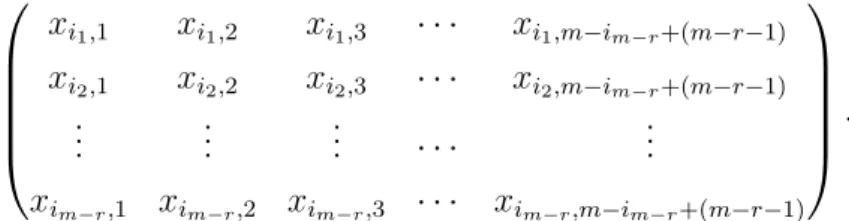
Cm,r =

        

x1 x2 x3 . . . xn

xr+1 xr+2 xr+3 . . . xr+n

x2r+1 x2r+2 x2r+3 . . . x2r+n

..

. ... ... . .. ...

x(m−1)r+1 x(m−1)r+2 x(m−1)r+3 . . . x(m−1)r+n

        

(1.1)

The extreme values r = 1 and r = m yield, respectively, the generic Hankel matrix and the generic matrix.

A crucial property proved in [16] is that the generic Hankel matrix of arbitrary sizem_×n is 1-generic. Using this property, it has been proved in [33] that the generic catalecticant matrix of arbitrary size and leap is 1-generic. This notion implies, in particular, that the determinant of a square such a matrix is irreducible (cf. the next theorem). Although the generic symmetric matrix is not an extreme case of a catalecticant, it is also 1-generic, which has been proven in [16, Proposition 4.4].

The following is a result of Eisenbud ([16, Theorem 2.1]) relating the property

l-generic of the matrix and the primeness of the r-minors ideal, for certain values of

r. With an appropriate language adaptation of the original notation, the part of the result we need reads as follows:

Proposition 1.2.3. One is given integers1_≤w_≤v. Let _G denote thew_×v generic matrix over a ground field. Let_M′ denote aw_×v matrix of linear forms in the entries of _G and let further _M denote a w_×v matrix of linear forms in the entries of _M′. Let there be given an integerk _≥1 such that _M′ is a(w₋k)-generic matrix and such that the vector space spanned by the entries of _M has codimension at most k ₋1 in the vector space spanned by the entries of _M′_{. Then the ideal} _I

k+1(M) is prime. It is known that the ideals of k-minors of the generic and generic symmetric matrices are prime ideals of codimension (m₋k+ 1)(m₋k+ 1) and m−₂k+2(see [13] and [27], respectively). In particular, the ideal of submaximal minors of a square generic matrix (respectively, a square generic symmetric matrix) is a prime ideal of codimension 4 (respectively, a prime ideal of codimension 3), regardless of the size of the matrix. An important property of the latter ideals is that they are (linearly presented) of linear type (see [25] for the generic case and [26] for the generic symmetric case).

In turn, the result [16, Proposition 4.3] ensures that the ideal of k-minors of the

m_×m generic Hankel matrix _Hm is also prime and of codimension 2m−2k+ 1. The

(20)

Theorem 1.2.4. Consider the generic Hankel matrix of arbitrary size which we write as follows:

Hj,2m−j :=

      

x1 x2 . . . x2m−j

x2 x3 . . . x2m−j+1

..

. ... . . . ... xj xm+1 . . . x2m−1

      

,

where j <2m. Then It(Hj,2m−j) =It(Ht,2m−t) for all t≤j ≤2m−t.

This property allows to reduce to the case of maximal minors. In this case, one may use the fact that the Hankel matrix specializes to the well-known specialization using only 2m₋2k+ 1 variables. In particular, in the case of the square Hankel matrix

Hm =Hm,m, its ideal of submaximal minors coincides with the ideal of maximal minors

of _Hm−1,m+1.

Several properties relating Im−1(Hm) to the gradient ideal J generated by the

partial derivatives of det(_Hm) are proved in [29]. One of these is that Im−1(Hm) is the

minimal component of the primary decomposition ofJ. In [28] it was proved that the

linear rankof J is 3 and conjectured thatJ is of linear type.

The following result, originally proved in [17] and independently obtained in [[28], Proposition 5.3.1], plays a role in looking at degenerations by zeros:

Proposition 1.2.5. Let _M denote a square matrix over R = k[x0, . . . , xn] satisfying

the following requirements:

• Every entry of _M is either 0 or xi for some i= 0, . . . , n;

• Any variable xi appears at most once on every row or column.

Let f = det(_M). Then, for each i = 0, . . . , n, the partial derivative of f with respect to xi is the sum of the (signed) cofactors of the entry xi, in all its appearances as an

entry of _M.

1.3 Homaloidal polynomials

Letk be an arbitrary field. For the purpose of the full geometric picture we may assumek to be algebraically closed. We denote by Pn ₌_Pn

k the n-th projective space,

where we naturally assume throughout thatn _≥1. A rational map _F : Pn

99K Pm is defined by m + 1 forms f = {f0, . . . , fm} ⊂

R := k[x] = k[x0, . . . , xn] of the same degree d ≥ 1, not all null. We often write

(21)

lost of generality be brought to satisfy the condition that gcd_{f0, . . . , fm} = 1 (in the

geometric terminology, _F has no fixed part). The common degree d of the forms fj is

the degree of _F and the ideal IF = (f0, . . . , fm) is called the base idealof F.

Theimageof _F is the projective subvariety W _⊂Pm _{whose homogeneous}

coordi-nate ring is the k-subalgebra k[f]_⊂R after degree renormalization. Write S :=k[f]_≃

k[y]/I(W), where I(W) _⊂ k[y] = k[y0, . . . , ym] is the homogeneous defining ideal of

the image in the embeddingW _⊂Pm_.

We say that_F isbirational onto the imageif there is a rational backwardsPm

99K

Pn _{such that the residue class}_g ₌_{_g

0, . . . , gn} ⊂S of a set of defining coordinates do

not simultaneously vanish and satisfy the relations

(g0(f) :· · ·:gn(f)) = (x0 :· · ·:xn), (f0(g) :· · ·:fm(g)) = (y0 :· · ·:ym).

When m = n and _F is a birational map of Pn_{, we say that} _F _{is a} _Cremona

map. An important class of Cremona maps of Pn _{comes off the so-called} _{polar maps}_,

that is, rational maps whose coordinates are the partial derivatives of a homogeneous polynomialf in the ring R=k[x0, . . . , xn]. More precisely:

Definition 1.3.1. Let f _∈ k[x] = k[x0, . . . , xn] be a square homogeneous polynomial

of degreed_≥2. Let

J =

∂f ∂x0

, . . . , ∂f ∂xn

⊂k[x].

the so calledgradient ideal of f. The rational map_Pf =

∂f

∂x0 :· · ·:

∂f ∂xn

is called the polar map defined by f. If _Pf is birational one says that f ishomaloidal.

We note that the image of this map is the subvariety on the target whose homo-geneous coordinate ring is given by the k-subalgebra k[∂f /∂x0, . . . , ∂f /∂xn] ⊂ k[x].

We call this variety of the polar variety.

A notable parallel construction is that of the dual variety V(f)∗ _{to the}

hyper-surface V(f). The homogeneous coordinate ring of its embedding in the usual dual coordinates can here be dealt with through thek-subalgebra

k[∂f /∂x0, . . . , ∂f /∂xn]

(f)_∩k[∂f /∂x0, . . . , ∂f /∂xn] ⊂

k[x] (f).

The following birationality criterion will be very useful in this work:

Theorem 1.3.2. [[12], Theorem 3.2] Let _F : Pn

99K Pm be a rational map given by m+ 1 forms g = _{g0, . . . , gm} of a fixed degree. If dim(k[g]) = n+ 1 and the linear

(22)

It is a classical result in characteristic zero that dim(k[f]) =n+ 1 coincides with the rank of the Jacobian matrix of f = _{f0, . . . , fn}. Assuming that the ground field

has characteristic zero, if the Hessian determinantH(f) does not vanish and the linear rank of the gradient ideal off is maximal, then f is homaloidal.

(23)

Chapter 2 Degenerations of the generic square

matrix

Throughout this chapter all matrices will have as entries either variables in a polynomial ring over a field or zeros, viewed as particular degenerations of the generic square matrix. Our goal is to understand the effect of such degenerations on the properties of underlying ideal theoretic structures such as the full determinant of the matrix, its gradient ideal, the associated polar map and its image, and the ideal of submaximal minors.

The degeneration types considered are: (1) degeneration by ”cloning” (repeating) a variable; (2) replacing a subset of entries with zeros, in a strategic layout;

2.1 Degeneration by cloning

More broadly, let A = (ai,j)1≤i,j≤m denote a m×m matrix where ai,j is either

a variable on a ground polynomial ring R = k[x] over a field k or ai,j = 0. Among

the simplest specializations is going modulo a binomial of the shapeai,j−ai′_,j′, where

ai,j 6=ai′_,j′ and a_i′_,j′ 6= 0. The idea is to replace a certain nonzero entrya_i′_,j′ (variable) by a different entryai,j (possibly zero), keeping ai,j as it was – somewhat like cloning

a variable, but keeping the mold. This has the effect of dropping the number of times a variable appears as an entry and often also dropping the total number of variables. It also seems natural to expect that the new cloning position should matter as far as the finer properties of the ideals are concerned.

(24)

G :=         

x1,1 x1,2 . . . x1,m−1 x1,m

x2,1 x2,2 . . . x2,m−1 x2,m

..

. ... . . . ... ...

xm−1,1 xm−1,2 . . . xm−1,m−1 xm−1,m

xm,1 xm,2 . . . xm,m−1 xm,m

        

, (2.1)

where the entries are independent variables over a fieldk.

Now, we distinguish essentially two sorts of cloning: the one that replaces an entryxi′_,j′ by another entry x_i,j such that i6=i′ and j 6=j′, and the one in which this replacement has either i=i′ _or _j ₌_j′_.

In the situation of the second kind of cloning, by an obvious elementary operation and renaming of variables (which is possible since the original matrix is generic), one can assume that the matrix is the result of replacing a variable by zero on a generic matrix. Such a procedure is recurrent, letting several entries being replaced by zeros. The resulting matrix along with its main properties will be studied in the Section 2.2. Therefore, this section will deal exclusively with the first kind of cloning – which, for emphasis, could be referred to asdiagonal cloning. Up to elementary row/column operations and renaming of variables, we assume once for all that the diagonally cloned matrix has the shape

GC :=         

x1,1 x1,2 . . . x1,m−1 x1,m

x2,1 x2,2 . . . x2,m−1 x2,m

..

. ... . . . ... ...

xm−1,1 xm−1,2 . . . xm−1,m−1 xm−1,m

xm,1 xm,2 . . . xm,m−1 xm−1,m−1         

, (2.2)

where the entry xm−1,m−1 has been cloned as the (m, m)-entry of the m×m generic matrix. Beyond a mere expression, the cloning imagery will remind us of a close interchange between properties associated to one or the other copy of the same variable in its position as an entry of the matrix.

2.1.1 Polar behavior

Throughout we set f := det(_GC) and let J = Jf denote the ideal generated by

the partial derivatives of f with respect to the variables of R, the polynomial ring in the entries of _GC over a ground field k. For convenience we call J the gradient ideal

of f – wishfully to distinguish it from the widely accepted terminology Jacobian ideal

(25)

Sticking to a more geometric terminology, we let the term polar be associated with the behavior of the gradient ideal as defining a rational map and the geometry of this map.

Theorem 2.1.1. Consider the diagonally cloned matrix as in (2.2). One has:

(i) f is irreducible.

(ii) The Hessian determinant H(f) does not vanish.

(iii) The linear rank of the gradient ideal of f is m2₋_{2 (}_{maximum possible}₎_. (iv) f is homaloidal.

Proof. (i) We induct on m, the initial step of the induction being subsumed in the general step.

By the Laplace expansion along the first row, one sees that

f =x1,1∆1,1+g,

where ∆1,1 is the determinant of the (m −1)×(m −1) cloned generic matrix ob-tained from _GC by omitting the first row and the first column. Note that both ∆1,1 and g belong to the subring k[x1,2, . . . , xm,m−1]. Thus, in order to show that

f is irreducible it suffices to prove that it is a primitive polynomial (of degree 1) in

k[x1,2, . . . , xm,m−1] [x1,1].

Now, on one hand, ∆1,1 is irreducible by the inductive hypothesis. Therefore, it is enough to see that ∆1,1 is not factor ofg. For this, one verifies their initial terms in the revlex monomial order: in(∆1,1) = x2,m−1. . . xm−1,2xm−1,m−1 and in(g) = in(f) =

x1,m−1. . . xm−1,1xm−1,m−1.

An alternative more sophisticated argument is to use that the idealP of submax-imal minors has codimension 4, as shown independently in the Theorem 2.1.2 (i) below. Since P = (J,∆m,m), as pointed out in the proof of the latter proposition, then J has

codimension at least 3. Therefore, the ringR/(f) is locally regular in codimension one, so it must be normal. Butf is homogeneous, hence irreducible.

(ii) Set v:=_{x1,1, x2,2, x3,3, . . . , xm−1,m−1} for the set of variables along the main diagonal. We argue by a specialization procedure, namely, consider the ring endomor-phism ϕ of R by mapping any variable in v to itself and by mapping any variable off

vto zero. Clearly, it suffices to show that by applying ϕ to the entries of the Hessian matrix _H(f) the resulting matrix has a nonzero determinant.

Note that the partial derivative of f with respect to any xi,i ∈ v coincides with

the (signed) cofactor of xi,i, for i ≤ m−2, while for i = m−1 it is the sum of the

(26)

By expanding each such a cofactor according to the Leibniz rule it is clear that it has a unique (nonzero) term whose support lies in v and, moreover, the remaining terms have degree at least 2 in the variables off v. Observe that in the two cofactors of xm−1,m−1 the terms whose support lies inv coincide.

Now, for xi,j ∈/ v, without exception, the corresponding partial derivative

co-incides with the (signed) cofactor. By a similar token, the Leibniz expansion of this cofactor has no term whose support lies in v and has exactly one nonzero term of degree 1 in the variables offv.

By the preceding observation, applying ϕ to any second partial derivative of f

will return zero or a monomial supported on the variables in v. Thus, the entries of the specialized Hessian matrix off, which we will denote _H′_{, are zeros or monomials}

supported on the variables inv.

To see that the determinant of this matrix _H′ _{is nonzero, consider the Jacobian}

matrix of the set of partial derivatives _{fv|v ∈ v} with respect to the variables in

v. Let M0 denote the specialization of this Jacobian matrix by ϕ, considered as a corresponding submatrix of_H′_{. Up to permutation of rows and columns of}_H′_{, we may}

write

H′ = M0 N

P M1

!

,

for suitableM1. Now, by the way the second partial derivatives off specialize via ϕ, as explained above, one must have N =P = 0. Therefore, det(_H′_{) = det(}_M

0) det(M1), so it remains to prove the nonvanishing of these two subdeterminants.

Now the first block is the Hessian matrix of the form

g :=

m_Y−2

i=1

xi,i

!

x2m−1,m−1. This is the product of the generators of the k-subalgebra

k[x1,1, . . . , xm−2,m−2, x2m−1,m−1]⊂k[x1,1, . . . , xm−2,m−2, xm−1,m−1].

Clearly these generators are algebraically independent overk, hence the subalgebra is isomorphic to a polynomial ring itself. Theng becomes the product of the variables of a polynomial ring overk. This is a classical homaloidal polynomial, hence we are done for the first matrix block.

As for the second block, by construction it has exactly one nonzero entry on each row and each column. Therefore, it has a nonzero determinant.

(iii) Let fi,j denote the xi,j-derivative of f and let ∆j,i stand for the (signed)

(27)

is the cofactor of xm−1,m−1 in the (m −1, m −1)-entry of GC (respectively, in the (m, m)-entry of _GC) and ∆j,i is the cofactor of xi,j on GC, for any (i, j) other than

(m₋1, m₋1) and (m, m).

The classical Cauchy cofactor formula

GC ·adj(_GC) = adj(_GC)_{· GC} = det(_GC)Im (2.3)

yields by expansion a set of linear relations involving the (signed) cofactors of_GC:

m

X

j=1

xi,j∆j,k = 0, for 1≤i≤m−1 and 1≤k ≤m−2 (k6=i); (2.4) m−1

X

j=1

xm,j∆j,k+xm−1,m−1∆m,k = 0, for 1≤k ≤m−2; (2.5) m

X

j=1

xi,j∆j,i= m

X

j=1

xi+1,j∆j,i+1, for 1≤i≤m−3; (2.6)

m

X

i=1

xi,k∆j,i= 0, for 1≤j ≤m−3 andj < k≤j+ 2; (2.7) m

X

i=1

xi,m−1∆m−2,i = 0; (2.8)

m_X−1

i=1

xi,m∆m−2,i+xm−1,m−1∆m−2,m = 0. (2.9)

Since fi,j = ∆j,i for every (i, j)6= (m−1, m−1) and the above relations do not

involve ∆m−1,m−1 or ∆m,m, then they give linear syzygies of the partial derivatives of

f.

In addition, (2.3) yields the following linear relations:

m_X−1

j=1

xm−1,j∆j,m+xm−1,m∆m,m = 0; (2.10) m_X−2

i=1

xi,m∆m−1,i+xm−1,m∆m−1,m−1+xm−1,m−1∆m−1,m = 0; (2.11) m_X−1

i=1

xi,m−1∆m,i+xm,m−1∆m,m= 0; (2.12) m_X−2

j=1

(28)

m

X

j=1, j6=m−1

xm−1,j∆j,m−1+xm−1,m−1∆m−1,m−1 =

m

X

j=1

xm−2,j∆j,m−2; (2.14)

m_X−1

j=1

xm,j∆j,m+xm−1,m−1∆m,m = m

X

j=1

xm−2,j∆j,m−2. (2.15) As fm−1,m−1 = ∆m−1,m−1 + ∆m,m, adding (2.10) to (2.11), (2.12) to (2.13) and

(2.14) to (2.15), respectively, outputs three new linear syzygies of the partial derivatives off. Thus one has a total of (m₋2)(m₋1) + (m₋3) + 2(m₋2) + 3 =m2₋_{2 linear} syzygies ofJ.

It remains to show that these are independent. For this we order the set of partial derivativesfi,j in accordance with the following ordered list of the entries xi,j:

x1,1, x1,2, . . . , x1,m x2,1, x2,2, . . . , x2,m . . . xm−2,1, xm−2,2, . . . , xm−2,m,

xm−1,1, xm,1 xm−1,2, xm,2 . . . xm−1,m−1, xm,m−1 xm−1,m.

Here, we traverse the entries along the matrix rows, left to right, starting with the first row and stopping prior to the row having xm−1,m−1 as an entry; then start traversing the last two rows along its columns top to bottom, until exhausting all variables.

We now claim that, the above sets of linear relations can be grouped into the following block matrix of linear syzygies:

                             ϕ1

0 ϕ2 . . .

..

. ... . .. ...

0 0 . . . ϕm−2 0m−1

2 0m2 . . . 0m2 ϕ32 0m−1

2 0m2 . . . 0m2 022 ϕ43

..

. ... . . . ... ... ... . ..

0m−1

2 0m2 . . . 0m2 022 022 . . . ϕ (m−1) (m−2) 0m−1

2 0m2 . . . 0m2 022 022 . . . 022 ϕm(m−1) 0m−1

1 0m1 . . . 0m1 021 021 . . . 012 021 xm−1,m xm,m−1 xm−1,m−1 0m−1

1 0m1 . . . 0m1 021 021 . . . 021 021 2xm−1,m−1 0 xm,m−1 0m−1

1 0m1 . . . 0m1 021 021 . . . 021 021 0 2xm−1,m−1 xm−1,m

                             .

We next explain the blocks of the above matrix:

• ϕ1 is the matrix obtained from the transpose GCt of GC by omitting the first column;

(29)

• ϕr+1 r =

xm−1,r xm−1,r+1

xm,r xm,r+1)

!

, forr = 2, . . . , m₋2;ϕm (m−1)=

xm−1,m−1 xm−1,m

xm,m−1 xm−1,m−1

!

;

• Each 0 under ϕ1 is a zero block of the size m×(m−1) and each 0 underϕi is a

zero block of the size m_×m for i= 2, . . . , m₋3 ;

• 0c

r denotes a zero block of size r×c, forr = 1,2 and c= 2, m−1, m.

Next, we justify why these blocks make up (linear) syzygies.

First, as already observed, the relations (2.4) through (2.15) yield linear syzygies of the partial derivatives off. Settingk= 1 in the relations (2.4) and (2.5) they can be written asPm_j₌₁xi,jf1,j = 0 for alli= 2, . . . , m−1 andPm_j₌₁−1xm,jf1,j+xm−1,m−1f1,m =

0, respectively. Ordering the set of partial derivatives fi,j as explained before, the

coefficients of these relations form the first matrix above

ϕ1 :=      

x2,1 x3,1 . . . xm−1,1 xm,1

..

. ... . . . ... ...

x2,m−1 x3,m−1 . . . xm−1,m−1 xm,m−1

x2,m x3,m . . . xm−1,m xm−1,m−1      

Note thatϕ1 coincides indeed with the submatrix of GCt obtained by omitting its first column.

Gettingϕk, fork = 2, . . . ., m−2, is similar, namely, use again relations (2.4) and

(2.5) retrieving a submatrix of _GCt excluding thekth column and replacing it with an extra column that comes from relation (2.6) takingi=k₋1.

Continuing, for each r = 2, . . . , m₋2 the block ϕr+1

r comes from the relation

(2.7) (setting j =r₋1) and ϕm

m−1 comes from the relations (2.8) and (2.9). Finally, the lower right corner 3_×3 block of the matrix of linear syzygies comes from the three last relations obtained by adding (2.10) to (2.11), (2.12) to (2.13) and (2.14) to (2.15). This proves the claim about the large matrix above. Counting through the sizes of the various blocks, one sees that this matrix is (m2 ₋₁₎_×₍_m2₋_{2). Omitting its} first row obtains a block-diagonal submatrix of size (m2 ₋₂₎_×₍_m2₋_{2), where each} block has nonzero determinant. Thus, the linear rank ofJ attains the maximum.

(iv) By (ii) the polar map of f is dominant. Since the linear rank is maximum by (iii), one can apply the Theorem 1.3.2 to conclude that f is homaloidal.

2.1.2 Primality

In this part we study the nature of the ideal of submaximal minors (cofactors) of

(30)

Theorem 2.1.2. Consider the matrix_GC as in (2.2), with m _≥3. Let P :=Im−1(GC)

denote its ideal of (m₋1)-minors. Then

(i) P is a Gorenstein prime ideal of codimension 4.

(ii) J has codimension 4 and P is the minimal primary component of J in R.

(iii) J defines a double structure on the variety defined by P, with a unique embed-ded component of codimension 4m₋5 supported on a linear space and no other embedded component of codimension _≤4m₋5.

(iv) Letting_D_i,j denote the cofactor of the(i, j)-entry of the generic matrix(yi,j)1≤i,j≤m,

the (m₋1)-minors ∆ =_{∆i,j} of GC define a birational map Pm

2₋₂

99KPm2−1

onto a hypersurface of degree m₋1 with defining equation Dm,m−Dm−1,m−1 and

inverse map defined by the linear system spanned by De :=_{Di,j|(i, j)6= (m, m)}

modulo _D_m,m₋_D_m₋₁_,m₋₁.

(v) J is not a reduction of P.

Proof. (i) Let _P denote the ideal of submaximal minors of the fully generic matrix (2.1). The linear form xm,m −xm−1,m−1 is regular on the corresponding polynomial ambient and also modulo_P as the latter is prime and generated in degree m₋1_≥2. Since_P is a Gorenstein ideal of codimension 4 by a well-known result (“Scandinavian complex”), then so isP.

In order to prove primality, we first consider the case m = 3 which seems to require a direct intervention. We will show more, namely, that R/P is normal – and, hence a domain asP is a homogeneous ideal. SinceR/P is a Gorenstein ring, it suffices to show thatR/P is locally regular in codimension one. For this consider the Jacobian matrix of P:

                 

x2,2 −x2,1 0 −x1,2 x1,1 0 0 0

x2,3 0 −x2,1 −x1,3 0 x1,1 0 0

0 x2,3 −x2,2 0 −x1,3 x1,2 0 0

x3,2 −x3,1 0 0 0 0 −x1,2 x1,1

x2,2 0 −x3,1 0 x1,1 0 −x1,3 0

0 x2,2 −x3,2 0 x1,2 0 0 −x1,3

0 0 0 x32 −x3,1 0 −x2,2 x21

0 0 0 x2,2 x2,1 −x3,1 −x2,3 0 0 0 0 0 2x2,2 −x3,2 0 −x2,3

                 

(31)

Direct inspection yields that the following pure powers are (up to sign) 4-minors of this matrix: x4

1,3,x42,1,x42,2,x42,3,x43,1 andx43,2. Therefore, the ideal of 4-minors of the Jacobian matrix has codimension at least 6 = 4 + 2, thus ensuring that R/P satisfies the condition (R1).

For m _≥ 4 we will apply the Theorem 1.2.3 in the case where _M′ ₌ _G _{is an}

m_×m generic matrix and _M=_GC is the cloned generic matrix as in the statement. In addition, we take k = m₋ 2, so k + 1 = m ₋1 is the size of the submaximal minors. Since m _≥ 4 and the vector space codimension in the theorem is now 1, one has 1_≤m₋3 =k₋1 as required. Finally, the m_×m generic matrix is m-generic as explained in [16, Examples, p. 548]; in particular, it is 2 =m₋(m₋2)-generic. The theorem applies to give that the idealP =Im−1(GC) is prime.

(ii) By item (i), P is a prime ideal of codimension 4. We first show that codim (J : P) > 4, which ensures that the radical of the unmixed part of J has no primes of codimension <4 and coincides with P – in particular, J will turn out to have codimension 4 as stated.

For this note thatP = (J,∆m,m), where ∆m,mdenotes the cofactor of the (m, m

)-entry of_GC. From the Cauchy cofactor formula we read the following relations:

m

X

j=1

xk,j∆j,m = 0, fork= 1, . . . , m−1; m_X−1

j=1

xm,j∆j,m+xm−1,m−1∆m,m = m

X

j=1

x1,j∆j,1;

m

X

i=1

xi,k∆m,i = 0, fork= 1, . . . , m−1.

Since the partial derivativefi,j off with respect to the variablexi,j is the (signed)

cofactor ∆j,i, with the single exception of the partial derivative with respect to the

variable xm−1,m−1, we have that the entries of the m-th column and the m-th row all belong to the ideal J : ∆m,m = J : P. In particular, the codimension of J : P is at

least 5, as needed.

In addition, since P has codimension 4 then J : P _6⊂ P. Picking an element

a_∈J :P _\P shows that PP ⊂JP. Therefore P is the unmixed part ofJ.

(32)

m

X

j=1,j6=m−1

xk,j∆j,m−1+xk,m−1∆m−1,m−1 = 0, fork = 1, . . . , m, (k6=m−1);

m

X

j=1,j6=m−1

xm−1,j∆j,m−1+xm−1,m−1∆m−1,m−1 =

m

X

j=1

x1,j∆j,1;

m

X

i=1,i6=m−1

xi,k∆m−1,i+xm−1,k∆m−1,m−1 = 0, fork = 1, . . . , m(k 6=m−1); Then as above we have that the entries of the (m₋1)-th column and the (m₋1)-th row belong to the idealJ : ∆m−1,m−1 =J :P.

From this, the variables of the last two rows and of the last two columns of _GC multiply P into J. As is clear that P is contained in the ideal generated by these variables it follows that P2 _⊂ _J _{(of course, this much could eventually be verified by} inspection). Therefore, the radical of J – i.e., the radical of the minimal primary part of J – is P.

(iii) By (ii), P is the minimal component of a primary decomposition of J. We claim thatJ :P is generated by the 4m₋5 entries of_GC off the upper left submatrix of size (m₋2)_×(m₋2). LetI denote the ideal generated by these entries.

As seen in the previous item, I _⊂ J : P. We now prove the reverse inclusion by writing I = I′ ₊_I′′ _{as sum of two prime ideals, where} _I′ _{(respectively,} _I′′_{) is the}

ideal generated by the variables on the (m₋1)-th row and on the (m₋1)-th column of _GC (respectively, by the variables on the m-th row and on the m-th column of

GC). Observe that the cofactors ∆i,j ∈ I′′ for all (i, j) 6= (m, m) and ∆i,j ∈ I′ for all

(i, j)₆= (m₋1, m₋1). Clearly, then ∆m,m ∈/ I′′ and ∆m−1,m−1 ∈/ I′. Let b_∈J :P =J : ∆m,m, say,

b∆m,m =

X

(i,j)6=(m−1,m−1)

ai,jfi,j+afm−1,m−1

= X

(i,j)6=(m−1,m−1)

ai,j∆j,i+a(∆m−1,m−1+ ∆m,m) (2.16)

for certain ai,j, a∈R. Then

(b₋a)∆m,m =

X

(i,j)6=(m−1,m−1)

ai,j∆j,i+a∆m−1,m−1 ∈I′′. Since I′′ _{is a prime ideal and ∆}

(33)

a=b₋cin (2.16) gives

(₋b+c)∆m−1,m−1 =

X

(i,j)6=(m−1,m−1)

ai,j∆j,i−c∆m,m ∈I′.

By a similar token, since ∆m−1,m−1 ∈/I′, then−b+c∈I′. Therefore

b=c₋(₋b+c)_∈I′′+I′ =I,

as required.

In particular, J : P is a prime ideal which is necessarily an associated prime of prime ofR/J. As pointed out, P _⊂J :P, hence J :P is an embedded prime of R/J. Moreover, this also givesP2 _⊂_J_{, hence}_J _{defines a double structure on the irreducible} variety defined byP.

Let_Qdenotes the embedded component ofJ with radicalJ :P and let_Q′ _denote

the intersection of the remaining embedded components of J. From J = P _{∩ Q ∩ Q}′

we get

J :P = (_Q:P)_∩(_Q′ :P),

in particular, passing to radicals,J :P _⊂√_Q′_{. This shows that}_Q_{is the unique}

embed-ded component of codimension_≤4m₋5 and the corresponding geometric component is supported on a linear subspace.

(iv) By Theorem 2.1.1 (ii), the polar map is dominant, i.e., the partial derivatives of f generate a subalgebra of maximum dimension (= m2 ₋_{1). Since} _J _⊂ _P _{is an} inclusion in the same degree, the subalgebra generated by the submaximal minors has dimension m2 ₋_{1 as well. On the other hand, since} _P _{is a specialization from the} generic case, it is linearly presented. Therefore, the minors define a birational map (see Theorem 1.3.2) onto a hypersurface. To get the defining equation of the latter we proceed as follows.

Write ∆j,i for the cofactor of the (i, j)-entry of GC. It suffices to show that

Dm,m−Dm−1,m−1 belongs to the kernel of the k-algebra map

ψ :k[yi,j|1≤i, j ≤m]→k[∆] =k[∆i,j|1≤i, j ≤m],

as it is clearly an irreducible polynomial.

Consider the following well-known matrix identity

adj(adj(_GC)) =fm−2_{· GC}_, _(2.17)

(34)

Looking at the (m₋1, m₋1)-entry and the (m, m)-entry of the right-hand side matrix we obviously see the same element, namely, fm−2_x

m−1,m−1.

As to the entries of the matrix on the left-hand side, for any (k, l), the (k, l)-entry is Dl,k(∆). Indeed, the (k, l)-entry of adj(adj(GC)) is the cofactor of the entry ∆l,k in

the matrix adj(_GC). Clearly, this cofactor is the (l, k)-cofactorDl,kof the generic matrix

(yi,j)1≤i,j≤m evaluated at ∆.

Therefore, we get (Dm,m−Dm−1,m−1)(∆) = 0, as required.

Finally, by the same token, from (2.17) one deduces that the inverse map has coordinates De :=_{Di,j|(i, j)6= (m, m)} modulo Dm,m−Dm−1,m−1.

(v) It follows from (iv) that the reduction number of a minimal reduction of P is

m₋2. Thus, to conclude, it suffices to prove thatPm−1 _6⊂_JPm−2_. We will show that ∆m−1

m,m ∈Pm−1 does not belong toJPm−2.

Recall from previous passages that J is generated by the cofactors

∆l,h, with (l, h)6= (m−1, m−1),(l, h)6= (m, m)

and the additional form ∆m,m+ ∆m−1,m−1. If ∆m−1

m,m ∈JPm−2, we can write

∆m_m,m−1 = X (l,h)6=(m−1,m−1)

(l,h)6=(m,m)

∆l,hQl,h(∆) + (∆m,m+ ∆m−1,m−1)Q(∆) (2.18) whereQl,h(∆) and Q(∆) are homogeneous polynomial expressions of degree m−2 in

the set

∆ =_{∆i,j|1≤i, j ≤m}

of the cofactors (generators ofP).

Clearly, this gives a polynomial relation of degree m₋1 on the generators of P, so the corresponding form of degreem₋1 ink[yi,j|1≤i, j ≤m] is a scalar multiple of

the defining equationH :=Dm,m−Dm−1,m−1 obtained in the previous item. Note that Hcontains only squarefree terms. We now argue that such a relation is impossible.

Namely, observe that the sum X

(l,h)6=(m−1,m−1) (l,h)6=(m,m)

∆l,hQl,h(∆)

does not contain any nonzero terms of the form α∆m−1

m,m or β∆m−1,m−1∆mm,m−2. In

(35)

a contradiction due to the squarefree nature ofH.

On the other hand, if c= 1 then we still have a polynomial relation ofP having a nonzero term ym−1,m−1ymm,m−2. Now, if m > 3 this is again a contradiction vis-`a-vis

the nature ofH as the nonzero terms of the latter are squarefree monomials of degree

m₋1 > 3₋1 = 2. Finally, if m = 3 a direct checking shows that the monomial

ym−1,m−1ym,m cannot be the support of a nonzero term in H. This concludes the

statement.

2.2 Degeneration by zeros

In this section, we look at the cloning degeneration where an entry is cloned along the same row or column of the original generic matrix. As mentioned before, up to elementary operations of rows and/or columns the resulting matrix has a zero entry. A glimpse of this first status has been tackled in [29, Proposition 4.9 (a)].

This procedure can be repeated to add more zeros. Aiming at a uniform treatment of all these cases, we will fix integersm, r with 1_≤r_≤m₋2 and consider the following degeneration of them_×m generic matrix:

                  

x1,1 . . . x1,m−r x1,m−r+1 x1,m−r+2 . . . x1,m−1 x1,m

..

. . . . ... ... ... . . . ... ... xm−r,1 . . . xm−r,m−r xm−r,m−r+1 xm−r,m−r+2 . . . xm−r,m−1 xm−r,m

xm−r+1,1 . . . xm−r+1,m−r xm−r+1,m−r+1 xm−r+1,m−r+2 . . . xm−r+1,m−1 0

xm−r+2,1 . . . xm−r+2,m−r xm−r+2,m−r+1 xm−r+2,m−r+2 . . . 0 0

..

. . . . ... ... ... . .. ... ... xm−1,1 . . . xm−1,m−r xm−1,m−r+1 0 . . . 0 0

xm,1 . . . xm,m−r 0 0 . . . 0 0

                  

(2.19)

Assuming m is fixed in the context, let us denote the above matrix by _DG(r).

2.2.1 Polar behavior

Theorem 2.2.1. Let R = k[x] denote the polynomial ring in the nonzero entries of

DG(r), with 1 _≤ r _≤ m₋2, let f := det(_DG(r)) and let J _⊂ R denote the gradient ideal off. Then:

(i) f is irreducible.

(ii) J has maximal linear rank.

(iii) The homogeneous coordinate ring of the polar variety of f in Pm2−(r+12 )−1 _{is a}

(36)

the analytic spread of J is m2 ₋_r₍_r_{+ 1)}_.

Proof. (i) Expanding the determinant by Laplace along the first row, we can write

f = x1,1∆1,1 +g, where ∆1,1 is the cofactor of x1,1 on DG(r). Clearly, both ∆1,1 and

g belong to the polynomial subring omitting the variable x1,1. Thus, in order to show that f is irreducible it suffices to prove that it is a primitive polynomial (of degree 1) ink[x1,2, . . . , xm,m−r][x1,1]. In order words, we need to check that no irreducible factor of ∆1,1 is a factor of g.

We induct on m _≥ r+ 2. If m = r + 2 then ∆1,1 = x2,mx3,m−1· · ·xm−1,3xm,2, while the initial term ofg in the revlex monomial order is

in(g) = in(f) =x1,mx2,m−1· · ·xm,1.

Thus, assume that m > r + 2. By the inductive step, ∆1,1 is irreducible being the determinant of an (m₋1)_×(m₋1) matrix of the same kind (samer). But deg(∆1,1) = deg(g)₋1. Therefore, it suffices to show that ∆1,1 is not a factor ofg. Supposing it were, we would get that f is multiple of ∆1,1 by a linear factor – this is clearly impossible.

Once more, an alternative argument is to use that the ideal J has codimension 4, as will be shown independently in Theorem 2.2.7 (ii). Therefore, the ring R/(f) is locally regular in codimension at least one, so it must be normal. Butfis homogeneous, hence irreducible.

(ii) The proof is similar to the one of Theorem 2.1.1 (iii), but there is a numerical diversion and, besides, the cases where r > m₋r₋1 and r _≤ m₋r₋1 keep slight differences.

Letfi,j denote thexi,j-derivative of f and let ∆j,i stand for the (signed) cofactor

of xi,j onDG(r). We first assume that r > m−r−1. The Cauchy cofactor formula

DG(r)_·adj(_DG(r)) = adj(_DG(r))_{· DG}(r) = det(_DG(r))Im

yields by expansion the following three blocks of linear relations involving the (signed) cofactors of_DG(r):

      

Pm

j=1xi,j∆j,k = 0 for 1≤i≤m−r, 1≤k≤m−r(k 6=i) Pm−l

j=1 xm−r+l,j∆j,k = 0 for 1≤l≤r, 1≤k ≤m−r

Pm

j=1xi,j∆j,i−Pmj=1xi+1,j∆j,i+1 = 0 for 1≤i≤m−r−1

(37)

( Pm

i=1xi,j∆k,i= 0 for 1≤j ≤m−r, 1≤k ≤m−r(k 6=j)

Pm−l

i=1 xi,m−r+l∆k,i = 0 for 1≤l≤2r−m+ 1, 1≤k≤m−r

(2.21)

with (m₋r)(m₋r₋1) + (m₋r)(2r₋m+ 1) =r(m₋r) such relations; and

( Pm−l

i=1 xi,m−r+l∆m−r+l,i−

Pm

j=1xi,1∆1,i= 0 for 1≤l ≤r−1 Pm−k

i=1 xi,m−r+k∆m−r+l,i= 0 for 1≤l ≤r−2, l+ 1 ≤k≤r−1 (2.22) with r(r₋1)/2 such relations.

Similarly, when r _≤ m₋r ₋1, the classical Cauchy cofactor formula outputs by expansion three blocks of linear relations involving the (signed) cofactors of_DG(r). Here, the first and third blocks are, respectively, exactly as the above ones, while the second one requires a modification due to the inequality reversal; namely, we get

( Pm

i=1xi,j∆k,i = 0 for 1≤j ≤r+ 1, 1≤k ≤r(k 6=j)

Pm

i=1xi,j∆k,i = 0 for 1≤j ≤r, r+ 1≤k ≤m−r,

(2.23)

with r(m₋r) such relations (as before).

Sincefi,j coincides with the (signed) cofactor ∆j,i, any of the above relations gives

a linear syzygy of the partial derivatives off. Thus one has a total of m2₋_rm₋_{1 +}

r(m₋r) +r(r₋1)/2 =m2₋ r+1 2

−1 linear syzygies of J. It remains to show that these are independent.

For this, we adopt the same strategy as in the proof of Theorem 2.1.1 (iii), whereby we list the partial derivatives according to the following ordering of the nonzero entries: we traverse the first row from left to right, then the second row in the same way, and so on until we reach the last row with no zero entry; thereafter we start from the first row having a zero and travel along the columns, from left to right, on each column from top to bottom, till we all nonzero entries are counted.

Thus, the desired ordering is depicted in the following scheme, where we once more used arrows for easy reading:

x1,1, x1,2, . . . , x1,m x2,1, x2,2, . . . , x2,m . . . xm−r,1, xm−r,2. . . , xm−r,m

xm−r+1,1, . . . , xm,1 xm−r+1,2, . . . , xm,2 . . . xm−r+1,m−r, xm−r+2,m−r, . . . ,

xm,m−r xm−r+1,m−r+1, . . . , xm−1,m−r+1 xm−r+1,m−r+2, . . . , xm−2,m−r+2

(38)

With this ordering the above linear relations translate into linear syzygies col-lected in the following block matrix

M=                                

ϕ1 . . .

0 ϕ2 . . .

..

. ... . .. ...

0 0 . . . ϕm−r

0m_r−1 0m_r . . . 0m_r ϕ1_r

0m−1

r 0mr . . . 0mr 0rr ϕ2r

..

. ... . . . ... ... ... . ..

0m−1

r 0mr . . . 0mr 0rr 0rr . . . ϕ

(m−r)

r

0m_r₋−₁1 0_rm₋₁ . . . 0m_r₋₁ 0r_r₋₁ 0r_r₋₁ . . . 0r_r₋₁ Φ1

0m_r₋−₂1 0m_r₋₂ . . . 0m_r₋₂ 0r_r₋₂ 0r_r₋₂ . . . 0r_r₋₂ 0r_r−₋1₂ Φ2

..

. ... ... ... ... ... ... ... ... ... . ..

0m₁−1 0m₁ . . . 0m₁ 0r₁ 0r₁ . . . 0₁r 0r₁−1 0₁r−2 . . . Φr−1

                                , where:

• ϕ1 is the matrix obtained from the transpose DG(r)t of DG(r) by omitting the first column

• ϕ2, . . . , ϕm−r are each a copy ofDG(r)t (up to column permutation);

• When r > m₋r₋1, ϕi

r is the r×r minor omitting the i-th column for i =

1, . . . , m₋r of the following submatrix of _DG(r):

              

xm−r+1,1 . . . xm−r+1,m−r xm−r+1,m−r+1 xm−r+1,m−r+2

..

. ... ... ... ...

xm−(2r−m+1),1 . . . xm−(2r−m+1),m−r xm−(2r−m+1),m−r+1 xm−(2r−m+1),m−r+2

xm−(2r−m+1)+1,1 . . . xm−(2r−m+1)+1,m−r xm−(2r−m+1)+1,m−r+1 xm−(2r−m+1)+1,m−r+2

..

. ... ... ... ...

xm−1,1 . . . xm−1,m−r xm−2,m−r+1 0

(39)

. . . xm−r+1,r+1

..

. ...

. . . xm−(2r−m+1),r+1

. . . 0

..

. ... . . . 0

. . . 0

              

.

When r_≤m₋r₋1,ϕi

ris the r×rminor obtained from the following submatrix

of _DG(r)

_





x

m−r+1,1

. . . x

m−r+1,r

x

m−r+1,r+1

..

.

..

.

..

.

..

.

m,1

. . .

x

m,r

x

m,r+1







by omitting thei-th column fori= 1, . . . , rand by omitting the (r+1)-th column for i=r+ 1, . . . , m₋r.

• Each 0 under ϕ1 is a zero block of the size m×(m−1) and each 0 underϕi is a

zero block of the size m_×m for i= 2, . . . , m₋r₋1 ;

• 0c

l denotes a zero block of size l×c.

• Φi is the (r−i)×(r−i) submatrix of DG(r) described bellow:

Φi =

     

xm−r+1,m−r+i xm−r+1,m−r+i+1 . . . xm−r+1,m−1

xm−r+2,m−r+i xm−r+2,m−r+i+1 . . . 0

..

. ... ... ...

xm−i,m−r+i 0 . . . 0

     

Next we justify why these blocks make up (linear) syzygies. As already explained, the relations in (2.20), (2.21) and (2.22) yield linear syzygies of the partial derivatives of f. Setting k = 1 in the first two relations of (2.20), the latter can be written as

Pm

j=1xi,jf1,j = 0, for i= 2, . . . , m−r, and Pmj=1−lxm−r+l,jf1,j = 0, for all l = 1, . . . , r.

Ordering the set of partial derivatives fi,j as explained before the coefficients of these

Open Degenerations of classical square matrices and their determinantal structure

Universidade Federal da Para´ıba

Universidade Federal de Campina Grande

Programa em Associa¸c˜

ao de P´

os Gradua¸c˜

ao em Matem´

atica

Doutorado em Matem´

atica

Degenerations of classical square

matrices and their

determinantal structure

Rainelly Cunha de Medeiros

Degenerations of classical square

matrices and their

determinantal structure

Rainelly Cunha de Medeiros

Prof. Dr. Aron Simis

Dedicat´

oria

Agradecimentos

Resumo

Abstract

Contents

Introduction

Chapter 1

Preliminaries

1.1

Recap of ideal theory

1.2

Recap of classical matrices

1.3

Homaloidal polynomials

Chapter 2

Degenerations of the generic square

matrix

2.1

Degeneration by cloning

2.1.1

Polar behavior

2.1.2

Primality

2.2

Degeneration by zeros

2.2.1

Polar behavior











x

. . . x

x

..

.

..

.

..

.

..

.

. . .

x

x











_