INTRODUCTION
The importance of quantitative genetic analysis for breeders is reflected by the large number of publications in which this approach is used. The diallel genetic design and its various modifications have been used by breeders to evalu-ate the potential of populations for intrapopulational im-provement and the usefulness of parents in interpopulational breeding programs, and to select inbred lines in hybrid de-velopment programs. Although several strategies for diallelic analysis have been proposed, few of them are commonly applied. The best-known methods are those developed by Jinks and Hayman (1953) and Hayman (1954a,b, 1958), both exclusively for homozygous parents, that by Griffing (1956a,b), valid for any species, that by Kempthorne and
Curnow (1961), for circulantdiallel cross, that by Gardner
and Eberhart (1966), normally used when the parents are open-pollinated populations, and those by Miranda Filho and Geraldi (1984) and Geraldi and Miranda Filho (1988), which are adaptations of the Gardner and Eberhart and the Griffing methods, respectively, for partial diallels. Of these, the Griffing (1956b) and Gardner and Eberhart (1966) methods are doubtless the most frequently applied.
The main reasons that justify the widespread use of the Griffing (1956b) method are its generality, since the par-ents can be clones, pure lines, inbred lines, or populations of a self-pollinated, cross-pollinated or intermediate spe-cies, and the ease of analysis and interpretation; the latter also characterizes the method developed by Gardner and Eberhart (1966). The genetic interpretation of parameters in the Gardner and Eberhart and the Griffing models and the
relationship between them have been discussed by Vencovsky (1970) and Cruz and Vencovsky (1989), thereby making the methods more accessible to breeders. However, the para-metric restrictions associated with these statistical models have not yet been examined in depth. Does the model neces-sarily have to be restricted? Do the restrictions satisfy the genetic parameters? Do the restrictions help to make the analysis and interpretation easier? The objective of this study was to answer these and other related questions.
MATERIAL AND METHODS
The same diallel analyzed by Gardner and Eberhart (1966) was considered here (Table I), although it is not an
ideal database because the tests on varietyheterosis and
specificheterosis are not significant at the 5% level.
Parametric values of the components of the Gardner and Eberhart (1966) model
We consider a polygenic system, with k genes, each with two allelic forms and no epistasis, and N non-endogamic populations in Hardy-Weinberg equilibrium involved in a diallel. The genotypic mean of population j (j = 1, 2 , ... , N) is
Mj = Σ mi + Σ [(2pij - 1)ai + 2(pij - p2ij)di] = m + vj
where mi is the mean of the genotypic values of the
ho-mozygotes relative to locus i, pij is the frequency in
popu-lation j of the locus i gene that increases traitexpression,
The parametric restrictions of the Gardner and Eberhart diallel
analysis model: heterosis analysis
José Marcelo Soriano Viana
Abstract
The parametric restrictions of the diallel analysis model of Gardner and Eberhart (analysis II) were studied in order to address the following questions: i) does the statistical model really have to be restricted? ii) Do the restrictions satisfy the genetic parameter values? iii) Do the restrictions make analysis and interpretation easier? Objectively, the answers to these questions are: i) no, ii) not all, and iii) they facilitate the analysis, but the interpretation is the same as for the unrestricted model. The main conclusion was that the restrictionsof the
Gardner and Eberhart’s estimators of the varietyheterosis effects, the specificheterosis effects and their variances, differ from those of the unrestricted model. Any analysis using the unrestricted model and that of Gardner and Eberhart should lead to the same inferences, at least for those based on assessment of the population effects expressed as deviations from the average value, theheteroses, the average heterosis and the varietyheteroses (the correlation between the estimates of the two models is 1). The limiting factor for the use of the unrestricted model is the lack of formulas for computing the sums of squares and for estimating the estimable function variances.
Departamento de Biologia Geral, Universidade Federal de Viçosa, 36571-000 Viçosa, MG, Brasil k
i = l k
i = l Gardner and Eberhart model related to specificheterosis effects, Σ S*
jj’ = 0 (j’ ≠ j), for all j, do not satisfy the parametric values. The N
ai is the difference between the genotypic value of the
ho-mozygotewith highest expression and mi, di is the
devia-tion due to dominance relative to locus i, and vj is the
ef-fect of population j.
Interpreting Mj is the same as interpreting vj because
m is a constant. The mean or the effect of a population is an indicator of its superiority relative to other populations in terms of the frequency of the favorable genes. If there is no predominant overdominance, the higher the genotypic mean or the effect of a population, the greater the frequen-cies of the genes that increase trait expression.
The average of the genotypic means of the diallel’s parents is
E(Mj) = M. = Σ mi + Σ [(2pi - 1)ai + 2(pi - p 2
i)di] = m + v.
where pi is the average frequency of the locus i gene that
increases trait expression,p2
i is the average genotypic
fre-quency of the homozygote of greatest expression relative
to locus i,and v. is the average of the population effects.
The genotypic mean of the hybrid between popula-tions j and j’ is
Mjj’ = Σ mi + Σ [(pij +pij’ - 1)ai + (pij + pij’ - 2pij pij’)di]
And theheterosisexpressed in the hybrid is
If there is dominance, the heterosisin the hybrid of
parents j and j’ indicates the degree of divergence between
them. The higher the value of aheterosis, the greater the
differences in gene frequency between the populations.
The mean of the heteroses expressedin the hybrids
of the genitor j (variety heterosis of parent j) is
Hj = E(Hjj’) = Σ (p2ij - 2pij pi.(j) + p2i.(j))di
where pi.(j) is the average frequency of the locus i gene that
increases trait expression in the diallel’s parents, except
the genitor j, and p2
i.(j) is the average genotypic frequency
of the homozygote with highest expression relative to lo-cus i in the diallel’s parents, except the genitor j.
Theheterosisof a population is null when the gene
frequencies in the population are equal to the average fre-quencies in the other diallel’s parents. Therefore, the higher
the absolutevalue of the heterosisof a population, the
greater the differences between the gene frequencies in the population and the average frequencies in the other diallel’s parents, i.e., the higher the divergence compared to the other genitors.
The averageheterosis is
H = E(Hjj’) = E(Hj) = M.. - M. = Σ 2p2i - Σ pij pi.(j) di
where
M.. = E(Mjj’) = Σ mi + Σ (2pi - 1)ai +
is the genotypic mean of the hybrids.
If there are differences in the gene frequencies
be-tween the diallel’s parents, the averageheterosis should be
used to evaluate the existence and predominant direction of deviations due to dominance. If the null hypothesis is confirmed, this proves to be the absence of dominance or bidirectional dominance. A value above zero means that the dominance effects are predominantly positive (the genes with some degree of dominance are those that increase trait expression). Unidirectional negative dominance is indi-cated if H is less than 0.
The genotypic mean of the hybrid between genitors j and j’ can be expressed as
Mjj’ = Σ mi + Σ [(2pij - 1)ai + 2(pij - p 2
ij)di] +
+ Σ [(2pij’ - 1)ai + 2(pij’ - p 2
ij’) di]
+ Σ (pij - pij’)2di = m + vj + vj’ + Hjj’
But,
H + Hj + Hj’ = Σ (pij - pij’)2di - Σ -2p2i +
+ Σ Σ 2pij pij’ + 2pij pi.(j) - p2i.(j) +
where Sjj’ is the specific heterosis of populations j and j’,
as defined by Gardner and Eberhart (1966). Finally,
Mjj’ = m + vj + vj’ + Hjj’ = m + vj + vj’ +
+ H + Hj + Hj’ + Sjj’
The discussion about specificheteroses is redundant
forheterosisanalysis involving the assessment of divergence
between genitor pairs, although it provides more
informa-tion thanthe Hjj’ values. For one gene and populations with
pij values of 0, 0.1, 0.2, 0.3, 0.4, 0.5, 0.6, 0.7, 0.8, 0.9 and 1,
the correlation betweenHjj’ and Sjj’ is approximately 0.84
for any degree of dominance (d/a ≠ 0). If there is
unidirec-tional negative dominance, the lowestSjj’ values identify the
k
i = l k
i = l
k
i = l k
i = l
k
i = l
Mj + Mj’
2
Hjj’ = Mjj’ - = Σ (pij - pij’) 2d
i
j fixed
k
i = l
2 N
N
j = l
+ 2pi - Σ pij pi.(j) di
1 2 1 2 1 2 1 2 k
i = l k
i = l
N
j = l
2 N
k
i = l
1 2
k
i = l
k
i = l
1 2
k
i = l
k
i = l
1 2 1 2 + k
i = l
k
i = l
1 N(N - 1)
2
N
j = l N
j’ = l <
populations with the greatest gene frequency differences between themselves and in relation to the average frequen-cies in the diallel’s parents. The highest values identify popu-lations with the smallest gene frequency differences, but with
gene frequencies different from the average frequenciesin
the diallel’s parents. When there is unidirectional positive
dominance, the lowest Sjj’ values are associated with
popu-lations having the smallest differences in gene frequencies, but which show differences in their gene frequencies
rela-tive to the average frequenciesin the diallel’s parents. The
highest values indicate populations with the greatest differ-ences in gene frequencies between themselves and in rela-tion to the parental group. Independent of the direcrela-tion of
the dominance effects, specificheterosis values close to
the average value (S.. = -2H) or near zero, when expressed as
deviations from the average effect, indicate populations with small gene frequency differences between themselves and
in relation to the average frequenciesin the parental group.
The specificheterosisof populations j and j’ is therefore an
indicator of the divergence between them (as Hjj’) and of
their divergence in relation to the diallel’s genitors.
The analysis of heteroses, varietyheteroses or
spe-cificheterosesis also redundant when assessing the
aver-ageheterosis for the predominant direction of deviations
due to dominance. If genes with some degree of dominance
increase trait expression, theheteroses andvariety
het-eroses are predominantly positive and the specific
het-eroses are all or nearly all negative.Negative heteroses,
varietyheteroses and positive specificheteroses indicate
unidirectional negative dominance.
Based on the previous results, the phenotypic means of population j and the hybrid from populations j and j’ are
Yj = m + vj + ej
and
Yjj’ = m + vj + vj’ + Hjj’ + ejj’ = m + vj + vj’ +
+ H + Hj + Hj’ + Sjj’ + ejj’
where ej and ejj’ are the average errors associated with the
phenotypic means of parent j and the hybrid between popu-lations j and j’.
The statistical models above are not those defined by Gardner and Eberhart (1966) because there are no restric-tions associated with them. These equarestric-tions therefore de-fine an unrestricted model. Normally, the unrestricted model is used to provide estimates of population genotypic
means, ofheteroses, of average heterosis, and of variety
and specific heteroses, while the restricted model of
Gardner and Eberhart (1966) is used to estimate popula-tion effects expressed as deviapopula-tions from the mean effect,
heteroses, averageheterosis, as well as the effects of
vari-etyand specificheteroses. Nevertheless, the
interpreta-tions are absolutely equivalent, as will be shown.
The genotypic means of a population and a hybrid can
be defined as shown below since E(Sjj’) = S.. = -2H:
Mj = m + vj± v. = (m + v.) + (vj - v.) = M. + v
* j
Mjj’= m + vj + vj’ + H + Hj + Hj’ + Sjj’± v.± S..
= (m + v.) + (vj - v.) + (vj’ - v.) + H + (Hj - H) +
+ (Hj’ - H) + (Sjj’ - S..) = M. + v
* j + v
* j’ +
+ H + H*
j + H *
j’ + S *
jj’
where v*
j = Mj - M. is the effect of population j expressed
as deviation from the average population effects, H*
j is the
effect of the heterosis of population j, and S*
jj’ is the effect
of the specificheterosis of populations j and j’.
Since M., H and S.. are constants, there is no
differ-ence at all between the interpretation of the estimates of
the population genotypic means, the varietyheterosesand
the specific heteroses in the unrestricted model, and the interpretation of the estimates of the population effects expressed as deviations from the average, the variety het-erosis effects and the specific hethet-erosis effects in the re-stricted model.
Thus, the statistical models that describe the pheno-typic means in the diallel table can be expressed as
Yj = M. + v*j + ej
and
Yjj’ = M. + v*j + v*j’ + Hjj’ + ejj’ = M. + v*j + v*j’ +
+ H + H*
j + H*j’ + S*jj’ + ejj’
The restricted model defined by these equations is not the same as that proposed by Gardner and Eberhart (1966) since the parametric restrictions are different. The restrictions necessarily associated with the restricted model described here are
(i) Σ v*
j = 0, (ii) Σ H*j = 0, and (iii) Σ Σ S*jj’ = 0
since E(v*
j) = E (H*j) = E(S*jj’) = 0, yielding three
restric-tions.
The restrictions of the Gardner and Eberhart (1966) model are
(i) Σ v*
j = 0, (ii) Σ H*j = 0, (iii) Σ Σ S*jj’ = 0,
giving N + 2 linearly independent restrictions.
The difference between the two restricted models lies 1
2 1 2
1 2
1 2
1 2
1 2
1 2
1 2
N
j = l
N
j = l
N
j = l N
j’ = l <
and (iv) Σ S*
jj’ = 0 (j’ ≠ j), for all j, N
j’ = l N
j = l
N
j = l
N
j = l N
j’ = l <
1 2
1 2 1 2
1 2
1 2
in the restrictions shown in item (iv), which do not satisfy
the parametric values of S*
jj’, since Σ S *
jj’ = H *
j (j’ ≠ j), for
all j. If the restrictions in (iv), of which N - 1 is linearly independent relative to the first three, are not coherent to the parametric values of the effects of specific heterosis, why were they considered by Gardner and Eberhart (1966)?
The answer is that without them, the normal equation
sys-tem X’Xβ° = X’Y is, as in the unrestricted model,
consis-tent and undetermined, which makes it impossible to de-fine formulas for estimating the variances of the effects and the contrasts of effects and for calculating the sums of squares. If the formulas could not be defined, the method-ology would have a more limited use, especially for soft-ware developers who are normally not specialists in quan-titative genetics and linear models. The problem of miss-ing formulas in the original paper, another fact that cer-tainly limited its use, was corrected in a later article (Gardner, 1967).
Since the restricted and unrestricted models de-scribed here are the same, the estimable functions in one are the estimable functions in the other. This means that in the unrestricted model, the population effects expressed as deviations from the mean effect can be analyzed, as can
be the effects of varietyand specificheteroses. In the
re-stricted model, population genotypic means and varietyand
specificheteroses can be analyzed. However, there are
dif-ferences between these models and that proposed by Gardner and Eberhart (1966), not in relation to the analysis of vari-ance nor to the testable hypotheses or to the estimable func-tions, but related to the estimators of several estimable functions and their variances. In any applied model, the tested hypotheses in the analysis of variance are:
1. H0(1): equality of the treatment means (parents and
hy-brids); testing this hypothesis implies testing that there are no differences in the gene frequencies between genitors (pij = pi for all i and j).
2. H0(2): equality of the population means (Mj = M. for all
j) or equality of the population effects (vj = v. for all j)
or nullity of the population effects expressed as
devia-tions from the average effect (v*
j = 0 for all j); if the
hypothesisH0(1) was rejected, testing this hypothesis
implies testing the equality of the effects of populations
with different genetic structures. The rejection ofH0(2)
indicates gene frequency differences between the diallel’s parents, but its acceptance does not indicate the contrary.
3. H0(3): nullity of the heteroses; if there are differences in
the gene frequencies between populations, testing this hypothesis is equivalent to testing that there is no
domi-nance (di = 0 for any i).
4. H0(4): nullity of the average heterosis; a redundant test in
relation to H0(3) although the statistics are associated with
different degrees of freedom for the numerator.
5. H0(5): equality of the varietyheteroses (Hj = H for all j)
or nullity of the variety heterosis effects (H*
j = 0 for all
j); if there are differences between the gene frequen-cies of the parents and if there is dominance, testing this hypothesis is to test that the degree of divergence of each population in relation to the other diallel’s par-ents is a constant.
6. H0(6): equality of the specificheteroses (Sjj’ = S.. = -2H
for all j and j’) or nullity of the specificheterosis
ef-fects (S*
jj’ = 0 for all j and j’); if there are differences
between the gene frequencies of the parents and if there is dominance, testing this hypothesis is to test that for all pairs of populations the magnitude of the divergence between themselves and between them and the diallel’s parents is a constant.
In relation to the estimable functions, the following must be emphasized: all the estimable functions in the unre-stricted model are also estimable in the Gardner and Eberhart (1966) model, even though the reciprocal is not true. Since in the latter the normal equation system is consistent and determined, the elements of the estimator of the parameter vector which are the estimators of the variety and specific heterosis effects are exclusive of this model.
RESULTS AND DISCUSSION
The analysis of variance of the diallel table (Table I) is valid for the unrestricted and the Gardner and Eberhart (analysis II) models (Table II). At the 5% level of
signifi-N
j’ = l
Table I - Mean grain yield (bushels/acre) of six corn
populations and their hybrids1.
1 - M 2 - HG 3 - GR 4 - BR 5 - K 6 - KII 1 - M 91.0 98.8 91.1 95.3 93.5 100.7
2 - HG 91.7 92.7 97.1 94.1 105.4
3 - GR 87.9 101.3 91.6 103.3
4 - BR 96.6 95.4 102.7
5 - K 91.3 101.6
6 - KII 96.2
1From Gardner and Eberhart (1966).
Table II - Diallel analysis of grain yield (bushels/acre) of six
corn populations and their hybrids, based on the unrestricted and Gardner and Eberhart (1966) models. Source of Degrees of Sum of Mean F Probability variation freedom squares square
Treatments 20 473.17 23.66 3.33 0.0002 Varieties 5 234.23 46.85 6.60 0.0001 Heterosis 15 238.94 15.93 2.24 0.0141 Average 1 115.44 115.44 16.26 0.0002
Variety 5 59.72 11.94 1.68 0.1527
Specific 9 63.78 7.09 1.00 0.4515
Error1 60 426.00 7.10
cance, the tests showed that i) there are differences in the gene frequencies between the populations, which justifies the inequality between their effects, ii) the deviations due to dominance contribute to the individual genotypic values for yield, iii) there are no differences between the variet-ies in their degree of divergence relative to the other diallel’s parents, and iv) there are no differences in the de-gree of divergence between population pairs and between the pairs and the diallel’s genitors. These results indicate that the populations chosen for an interpopulational im-provement program should be those with higher frequen-cies of the genes that increase yield.
In the analysis according to the Gardner and Eberhart (1966) model, the variety sum of squares is the sum of squares attributable to the hypothesis of equality of the population effects, allowing for an absence of dominance
or the presence of only averageheterosis. Consequently, it
is only possible to use the quotient between the variety
mean square and the error mean square to test the H0(2)
hy-pothesis if there is no dominance or if there is only
aver-ageheterosis. Indeed this was the situation described by
Gardner and Eberhart (1966). Therefore, the test is adequate and has also been considered in the unrestricted model. If there were evidence of differences between the variety
heteroses and/or the specificheteroses, the correct
statis-tic for the test of the hypothesis of equality for the popula-tion effects would be F = 11.195/7.1 = 1.58 (probability = 0.18). The problem in this case is to obtain the adequate variety sum of squares (55.975 in the example given) since the latter is not orthogonal relative to the heterosis sum of squares, and it is therefore not possible to define an ex-pression for its calculation.
The estimates of the main estimable functions in the unrestricted model, which are also estimable, as mentioned
before, in the Gardner and Eberhart (1966)model, their
variances and the variances of the contrasts between them are shown in Tables III and IV. As stated above, analyzing the estimates of the population genotypic means, and of
the variety and specificheteroses is equivalent to
analyz-ing the estimates of the population effects expressed as deviations relative to the average effect, the variety
het-erosis effects and the specificheterosis effects, because
the correlation between the function estimates is 1. These results showed that the populations 4 and 6 are superior to the others in terms of frequency of favorable genes and can be used in intrapopulational improvement programs, and that the dominance effects are predominantly positive. As there are no significant differences between
the variety heteroses and the specificheteroses, both can
also be used in a reciprocal recurrent selection program. The heterosis estimates show that the populations with the greatest gene frequency differences are 2 and 6, and 3 and 6. If the hypotheses of equality of the variety and specific heteroses were rejected, the following inferences would still hold: i) population 6 is the most divergent from the other parents, and would necessarily be chosen for an
Table III - Estimates of the population genotypic means (Mj), variety
heteroses (Hj), population effects expressed as deviations from the average effect (v*
j), variety heterosis effects (H*j) and the variances of these and other linear combinations of the parameters,
relative to grain yield (bushels/acre), in the unrestricted model.
Population Mj Hj v*j H*j
1 91.0 4.01 -1.45 -1.18
2 91.7 5.47 -0.75 0.28
3 87.9 5.37 -4.55 0.18
4 96.6 4.25 4.15 -0.94
5 91.3 3.25 -1.15 -1.94
6 96.2 8.79 3.75 3.60
V(Mj) = 7.10 V(Hj) = 3.55 V(v*
j) = 5.92 V(H*
j) = 1.89
V(vj - vj’) = V(Mj - Mj’) = V(v *
j - v *
j’) = 14.20 V(Hj - Hj’) = V(H
* j - H
* j’) = 4.54
^ ^
^ ^
^ ^ ^ ^
^ ^
^ ^
^ ^ ^ ^
^
^
^ ^ ^ ^
^ ^ ^ ^ ^
^ ^
^ ^
interpopulational improvement program, ii) the populations which diverge most between themselves and in relation to the parental group are 3 and 4, and 1 and 2, iii) populations 1 and 3, and 2 and 3 diverge at a small rate, but have differ-ent gene frequencies relative to the average frequencies in
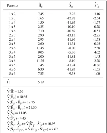
TableIV - Estimates of the heteroses (Hjj’), average heterosis (H),
specific heteroses (Sjj’), specific heterosis effects (S *
jj’) and the variances of these and other linear combinations of the parameters,
relative to grain yield (bushels/acre), in the unrestricted model.
Parents Hjj’ Sjj’ S
* jj’
1 x 2 7.45 -7.22 3.16
1 x 3 1.65 -12.92 -2.54
1 x 4 1.50 -11.95 -1.57
1 x 5 2.35 -10.10 0.28
1 x 6 7.10 -10.89 -0.51
2 x 3 2.90 -13.13 -2.75
2 x 4 2.95 -11.96 -1.58
2 x 5 2.60 -11.31 -0.93
2 x 6 11.45 -8.00 2.38
3 x 4 9.05 -5.76 4.62
3 x 5 2.00 -11.81 -1.43
3 x 6 11.25 -8.10 2.28
4 x 5 1.45 -11.24 -0.86
4 x 6 6.30 -11.93 -1.55
5 x 6 7.85 -9.38 1.00
H 5.19
V(H) = 1.66 V(Hjj’) = 10.65 V(Hjj’ - Hjj”) = 17.75 V(Hjj’ - Hj”j’”) = 21.30 V(Sjj’) = 11.08 V(S*
jj’) = 4.45
V(Sjj’ - Sjj”) = V(S*jj’ - S*jj”) = 10.93 V(Sjj’ - Sj”j’”) = V (S*jj’ - S*j”j’”) = 7.67
^
^
^ ^
^ ^ ^
^ ^
^
^ ^
^ ^ ^
^ ^ ^
^ ^
^ ^
^ ^ ^ ^ ^
^ ^ ^ ^ ^
^
the parental group, and iv) the gene frequencies in popula-tions 1 and 5, and 1 and 6 come close to the average values for the diallel’s parents.
Tables V and VI show the estimates of the parameters for the model developed by Gardner and Eberhart (1966). The differences in adjustment relative to the unrestricted model are limited to the estimates of the variety and
spe-cific heterosiseffects and their variances. The variances
associated with the estimates of variety heterosis and their contrasts are considerably smaller for the functions ob-tained by adjusting the unrestricted model. On the other hand, the estimates of the variances of the specific hetero-sis effects and their contrasts are smaller for the functions
normally estimated by the Gardner and Eberhart (1966) model. However, the correlation between the estimated
values of H*
j and S *
jj’ are of high magnitude (1 and 0.96,
respectively). Hence, the inferences that can be established tend to be the same as those obtained previously. If there were any statistical difference between the specific het-eroses, only one inference would not conform with the
results of the unrestricted model: the estimates of S*
jj’
in-dicate that populations 4 and 5, and 2 and 5 are the least divergent between themselves and in relation to the paren-tal group.
CONCLUSIONS
Gardner and Eberhart (1966) model do not satisfy the para-metric values of the specific heterosis effects. Conse-quently, the estimators of the effects of variety heterosis, specific heterosis and their variances differ from those of the unrestricted model. Analyses using the unrestricted and the Gardner and Eberhart (1966) models should lead to the same inferences, at least in the assessment of population effects expressed as deviations from the average effect, the heteroses, the average heterosis and the variety het-eroses (the correlation between the estimates of the two models is 1). The use of the unrestricted model is limited by the lack of formulas for calculating the sums of squares and the variance estimates for estimable functions, although this does not exclude the possibility of developing the ap-propriate software for analysis. In conclusion, it is gener-ally quite safe to use the Gardner and Eberhart model.
RESUMO
O objetivo deste trabalho foi discutir as restrições paramétricas do modelo de análise dialélica de Gardner & Eberhart (análise II), visando responder às seguintes questões, entre outras: i) o modelo estatístico tem que ser restrito?; ii) as restrições satisfazem os valores dos parâmetros genéticos?, e iii) elas tornam a análise e a interpretação mais fáceis? Objetivamente, estas questões podem ser assim respondidas: i) não; ii) nem todas, e iii) a análise sim, mas a interpretação é a mesma do modelo irrestrito.
As principais conclusões são: as restrições Σ S*
jj’ = 0 (j’ ≠ j),
para todo j, do modelo de Gardner & Eberhart não satisfazem os valores paramétricos dos efeitos de heterose específica; em conseqüência, os estimadores dos efeitos de heterose de população, dos efeitos de heterose específica e de suas variâncias diferem daqueles do modelo irrestrito; as análises considerando os modelos irrestrito e de Gardner & Eberhart devem conduzir às mesmas inferências, pelo menos em relação às decorrentes da avaliação dos efeitos de população expressos como desvios em torno do efeito médio, das heteroses, da heterose média e das heteroses varietais (a correlação entre as estimativas dos dois modelos é 1); o fator que limita o uso do modelo irrestrito é a inexistência de fórmulas para o cálculo das somas de quadrados e
Table VI - Estimates of the heteroses (Hjj’; values below the diagonal),
specific heterosis effects (S*
jj’; values above the diagonal), average heterosis (H) and the variances of these and other linear combinations
of the parameters, relative to grain yield (bushels/acre), based on the Gardner and Eberhart (1966) model.
Parents 1 2 3 4 5 6
1 3.385 -2.290 -1.040 1.060 -1.115
2 7.45 -2.865 -1.415 -0.515 1.410
3 1.65 2.90 4.810 -0.990 1.335
4 1.50 2.95 9.05 -0.140 -2.215
5 2.35 2.60 2.00 1.45 0.585
6 7.10 11.45 11.25 6.30 7.85 H = 5.19
V(H) = 1.66 V(Hjj’) = 10.65 V(Hjj’ - Hjj”) = 17.75 V(Hjj’ - Hj”j’”) = 21.30 V(S*
jj’) = 4.26 V(S*
jj’ - S*jj”) = 10.65 V(S*
jj’ - S*j”j’”) = 7.01
^ ^
^
^
^ ^
^ ^
^ ^ ^
^ ^ ^
^ ^
^ ^ ^
^ ^ ^
Table V - Estimates of the population effects expressed as
deviations from the average effect (v*
j), variety heterosis effects (H*
j) and the variances of these and other linear combinations of the parameters, relative to grain yield (bushels/acre), based
on the Gardner and Eberhart (1966) model.
Population v*
j H*j
1 -1.45 -1.475
2 -0.75 0.350
3 -4.55 0.225
4 4.15 -1.175
5 -1.15 -2.425
6 3.75 4.500
V(v* j) = 5.92 V(H*
j) = 2.96 V(v*
j - v*j’) = 14.20 V(H*
j - H*j’) = 7.10
^ ^
^ ^
^ ^ ^ ^
^ ^ ^
^ ^ ^
N
j’ = l N
j’ = l
The restrictions Σ S*
das estimativas das variâncias das funções estimáveis, embora isto não impossibilite o desenvolvimento de ‘software’ para automa-tização da análise.
REFERENCES
Cruz, C.D. and Vencovsky, R. (1989). Comparação de alguns métodos de
análise dialélica. Rev. Bras. Genet. 12: 425-438.
Gardner, C.O. (1967). Simplified methods for estimating constants and
computing sums of squares for a diallel cross analysis. Fitotec. Lati-noam. 4: 1-12.
Gardner, C.O. and Eberhart, S.A. (1966). Analysis and interpretation of
the variety cross diallel and related populations. Biometrics 22: 439-452.
Geraldi, I.O. and Miranda Filho, J.B. de (1988). Adapted models for the
analysis of combining ability of varieties in partial diallel crosses. Rev. Bras. Genet. 11: 419-430.
Griffing, B. (1956a). A generalized treatment of the use of diallel crosses in
quantitative inheritance. Heredity 10: 31-50.
Griffing, B. (1956b). Concept of general and specific combining ability in
relation to diallel crossing system. Aust. J. Biol. Sci. 9: 463-493.
Hayman, B.I. (1954a). The analysis of variance of diallel tables. Biometrics
10: 235-244.
Hayman, B.I. (1954b). The theory and analysis of diallel crosses. Genetics
39: 789-809.
Hayman, B.I. (1958). The theory and analysis of diallel crosses. II.
Genet-ics 43: 63-85.
Jinks, J.L. and Hayman, B.I. (1953). The analysis of diallel crosses. Maize
Genet. Coope vration News Lett. 27: 48-54.
Kempthorne, O. and Curnow, R.N. (1961). The partial diallel cross.
Bio-metrics 17: 229-250.
Miranda Filho, J.B. de and Geraldi, I.O. (1984). An adapted model for the
analysis of partial diallel crosses. Rev. Bras. Genet. VII: 677-688.
Vencovsky, R. (1970). Alguns aspectos teóricos e aplicados relativos a
cruzamentos dialélicos de variedades. Livre Docência thesis, ESALQ/ USP, Piracicaba, SP.