OSD
9, 3049–3070, 2012Island and ocean sea-level
J. Williams and C. W. Hughes
Title Page
Abstract Introduction
Conclusions References
Tables Figures
◭ ◮
◭ ◮
Back Close
Full Screen / Esc
Printer-friendly Version Interactive Discussion
Discussion
P
a
per
|
Dis
cussion
P
a
per
|
Discussion
P
a
per
|
Discussio
n
P
a
per
|
Ocean Sci. Discuss., 9, 3049–3070, 2012 www.ocean-sci-discuss.net/9/3049/2012/ doi:10.5194/osd-9-3049-2012
© Author(s) 2012. CC Attribution 3.0 License.
Ocean Science Discussions
This discussion paper is/has been under review for the journal Ocean Science (OS). Please refer to the corresponding final paper in OS if available.
The coherence of small island sea-level
with the wider ocean: a model study
Joanne Williams and Christopher W. Hughes
National Oceanography Centre, 6 Brownlow St, Liverpool L3 5DA, UK
Received: 29 August 2012 – Accepted: 12 September 2012 – Published: 26 September 2012
Correspondence to: J. Williams ([email protected])
OSD
9, 3049–3070, 2012Island and ocean sea-level
J. Williams and C. W. Hughes
Title Page
Abstract Introduction
Conclusions References
Tables Figures
◭ ◮
◭ ◮
Back Close
Full Screen / Esc
Printer-friendly Version Interactive Discussion
Discussion
P
a
per
|
Dis
cussion
P
a
per
|
Discussion
P
a
per
|
Discussio
n
P
a
per
|
Abstract
Studies comparing tide gauge measurements with sea level from nearby satellite al-timetry have shown good agreement for some islands, and poor agreement for others, though no explanation has been offered. Using the 1/12◦OCCAM ocean model, we in-vestigate the relationship between sea level at small, open-ocean islands, and offshore
5
sea level. For every such island or seamount in the model, we compare the shallow-water sea level with the steric and bottom pressure variability in a neighboring ring of deep water. We find a latitude-dependent range of frequencies for which off-shore sea level is poorly correlated with island sea level. This poor coherence occurs in a spec-tral region for which steric signals dominate, but are unable to propagate as baroclinic
10
Rossby waves. This mode of decoupling does not arise because of island topography, as the same decoupling is seen between deep ocean points and surrounding rings.
1 Introduction
Tide gauges are necessarily situated on the coast and in using tide-gauge data to draw inferences about the deeper ocean some assumptions must be made. Satellite
15
altimetry, by contrast, has until recently performed poorly at the coast (Vignudelli et al., 2011). How does sea-level at islands relate to that offshore? This question matters not only to island communities but also because island tide gauges play a particularly important role in satellite altimetry calibration (Leuliette et al., 2004). It may also be significant for reconstructing global sea levels from historic tide gauge records. It has
20
been addressed to some extent by Vinogradov and Ponte (2011), who compared tide gauge records to nearby sea-surface height derived from Topex/Poseidon altimetry. “Nearby” here refers to altimetry from within 180 km, also usually more than 200 m deep. They find the percentage of variance in near-gauge altimetry data explained by the gauge is high (>80 %) for most Pacific islands and Indian Ocean sites, but low
25
OSD
9, 3049–3070, 2012Island and ocean sea-level
J. Williams and C. W. Hughes
Title Page
Abstract Introduction
Conclusions References
Tables Figures
◭ ◮
◭ ◮
Back Close
Full Screen / Esc
Printer-friendly Version Interactive Discussion
Discussion
P
a
per
|
Dis
cussion
P
a
per
|
Discussion
P
a
per
|
Discussio
n
P
a
per
|
Eastern South Pacific – see Fig. 6 in their paper. They also hint at improved correlations when timeseries are averaged over longer periods – 2 and 3 yr.
There are three ways in which coastal sea level can be decoupled from nearby deep water variability. First: there can be additional variability in shallow water, resulting from local effects of wind stress and atmospheric pressure. Second: deep water signals,
5
which are often primarily steric (density-related), can fail to penetrate to the coast (as bottom pressure signals; they cannot remain as steric signals in shallow water) be-cause the interaction of density with topography can induce alongshore currents which block the propagation of a pressure signal onshore. Third: it may simply be the case that the offshore variability does not propagate in an organized manner, and therefore
10
is not strongly correlated with any nearby variability, coastal or otherwise.
The first two of these mechanisms appear to be operating on some continental coasts, as illustrated in spectra of sea level variability in the range of periods 2–24 weeks by Hughes and Williams (2010). These show several regions where variability in shallow water is dominated by high frequency content, and that in deeper water by
15
low frequencies, with the two separated by low variability along the shelf edge. Thus, the deep water variability does not penetrate onto the shelf, and there is additional variability on the shelf with a spectrum representative of wind-driven processes.
Bingham and Hughes (2012) looked at continental coasts in the OCCAM 1/12◦
model, reconstructing coastal sea level using various approximations. “Approximation
20
A” in their paper, was that sea-surface height is spatially constant near the coast, ∇p0=0, so the tide gauge can be approximated by steric height at a nearby point.
This only does well near the equator, with performance dropping poleward of about 20◦, particularly on the western ocean boundaries. “Approximation C” in their paper was that the horizontal gradient of pressure anomaly at the bottom is zero, ie there
25
OSD
9, 3049–3070, 2012Island and ocean sea-level
J. Williams and C. W. Hughes
Title Page
Abstract Introduction
Conclusions References
Tables Figures
◭ ◮
◭ ◮
Back Close
Full Screen / Esc
Printer-friendly Version Interactive Discussion
Discussion
P
a
per
|
Dis
cussion
P
a
per
|
Discussion
P
a
per
|
Discussio
n
P
a
per
|
disrupt the link between coastal and deep ocean sea level, even on interannual time scales.
For small islands, we might expect both of these mechanisms to be less effective. The closed, short topographic contours around an island may present less of a barrier to signal propagation, and the shallow water area over which wind stress acts will be
5
smaller, producing less additional local variability. Nonetheless, in this model study we do see significant decoupling for many islands, and the much greater data availability in the model compared with the limited number of tide gauge records available in the real world allows us to investigate the spatial and spectral dependence of this decoupling in more detail. We find evidence for the importance of the third decoupling mechanism,
10
which does not depend on the reference point being an island, or in shallow water, but operates at all open ocean points.
2 Methods
For this paper sea-surface height, steric height and bottom pressures are calculated from run 401 of the OCCAM 1/12◦ model (Marsh et al., 2009), sampled as 5-day
15
means over the years 1988–2004. We will consider variability of inverse-barometer corrected sea-level h to be the sum of variation in terms p and φ associated with bottom pressurepband steric variations, respectively, where
h=p+φ= pb
ρ0g
−
0 Z
−H
ρgdz. (1)
ρis density (withρ0 the model’s Boussinesq reference density), gis the acceleration
20
due to gravity,zis the vertical coordinate andH is ocean depth.
OSD
9, 3049–3070, 2012Island and ocean sea-level
J. Williams and C. W. Hughes
Title Page
Abstract Introduction
Conclusions References
Tables Figures
◭ ◮
◭ ◮
Back Close
Full Screen / Esc
Printer-friendly Version Interactive Discussion
Discussion
P
a
per
|
Dis
cussion
P
a
per
|
Discussion
P
a
per
|
Discussio
n
P
a
per
|
“continental” and New Zealand for being too large, but Fiji is included. There is no re-quirement for there to actually be any land, so some small sea-mounts are included. With this generous definition we find islands in much of the ocean, though there are few in the deep East Pacific (the distribution can be seen in later figures).
For each island we compare sea-surface height (h) averaged over this onshore-area
5
withhand its steric (φ) and bottom pressure (p) components, averaged over a “ring” around the island, defined as all points deeper than 3000 m and closer than 2.5◦latitude and longitude (∼200 km at mid-latitudes) to the island centre.
To establish whether any effects are due to the island depth or simply distance, we also define “control islands” as 0.75◦×0.75◦ squares of water over 3000 m deep and
10
compare sea-level there to the surrounding squares between widths 0.75◦ and 2.5◦ (intermediate ring) and between widths 2.5◦and 5◦ (distant ring).
3 Results
3.1 Global mean spectra
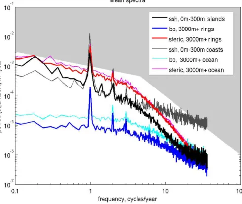
Firstly, we compare the spectra of sea-level signals averaged over all the islands with
15
that for deep oceans and continental coasts. The deep waterφvariability (heavy and light red, Fig. 1) has a spectrum approximately proportional toσ−1/2, steepening be-yond σ−2 at frequencies (σ) greater than 3 cycles/year. Steric variability has much greater power than bottom pressurep (heavy and light blue) in deep water, which has a more gently-sloping spectrum. The near-islandp spectrum is a little less energetic
20
than that for the deep ocean as a whole but very similar in shape. The h signal at the islands (heavy black), has a spectrum similar in character but reduced in power compared to the deepφ, suggesting an influence of nearby steric variability on island sea level, but a degree of decoupling resulting in reduced power. The islandh spec-trum is very close to the continental coastal h (light black) between about 4 months
25
OSD
9, 3049–3070, 2012Island and ocean sea-level
J. Williams and C. W. Hughes
Title Page
Abstract Introduction
Conclusions References
Tables Figures
◭ ◮
◭ ◮
Back Close
Full Screen / Esc
Printer-friendly Version Interactive Discussion
Discussion
P
a
per
|
Dis
cussion
P
a
per
|
Discussion
P
a
per
|
Discussio
n
P
a
per
|
energetic. This corresponds to the “blue” high-frequency spectra seen on the continen-tal coasts in the altimetry spectral maps of Hughes and Williams (2010). The greater high-frequency energy in coastal shallow water is due, in part at least, to the greater ef-fect on sea level of wind over shallow water than over deep water. The rapid drop-offof the island sea level spectrum at these high frequencies is consistent with this process
5
being a much less important source of decoupling at islands than on broad continental shelves, though we should note that the limitations of model resolution may lead to an underestimate of the energy in small-scale, local processes. The island sea level spec-trum also approaches the near-island steric specspec-trum at the longest timescales, unlike the continental coastal sea level spectrum, perhaps suggesting that the decoupling
10
reduces at the longest time scales.
The shapes of the spectra suggest that nearby steric-height signals do directly in-fluence coastal island sea level, but that deep bottom pressure signals become the dominant influence at high frequency. But all these interpretations remain tentative when based on globally-averaged spectra. A more detailed analysis is needed in order
15
to understand the processes.
3.2 Relationship between island and off-shore sealevel
3.2.1 For islands
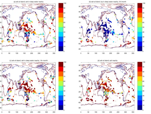
To investigate geographically-varying effects, we plot in Fig. 2a the percentage of vari-ance of the islandhsignal explained byhin the surrounding ring of deep water. A
lati-20
tude dependence emerges, with much higher variance explained at the equator, drop-ping with latitude, and rising again in the Southern Ocean. A similar plot (not shown) forp at the island explained by hoffshore is nearly identical to this, and a plot of h
explained byφoffshore is also very alike, with changes mainly in the Southern Ocean. Less than 5 % of overall island variability is explained by the offshore p, except in the
25
OSD
9, 3049–3070, 2012Island and ocean sea-level
J. Williams and C. W. Hughes
Title Page
Abstract Introduction
Conclusions References
Tables Figures
◭ ◮
◭ ◮
Back Close
Full Screen / Esc
Printer-friendly Version Interactive Discussion
Discussion
P
a
per
|
Dis
cussion
P
a
per
|
Discussion
P
a
per
|
Discussio
n
P
a
per
|
What is the timescale upon which the offshoreφsignal can approximate the island
h? If we filter each signal to pass periods<6 months before calculating the percentage of variance (not shown) we find that at the shorter time scales the islandh variance explained by the offshore φ drops from a maximum of about 90 % at the equator to a maximum of 80 %. The latitude dependence remains, and polewards of 20◦ latitude
5
there are few islands for which the off-shore φalone explains more than about 25 % of the variance of the island h signal. Offshore φ does almost as well as offshore h
except in the Southern Ocean where it is the offshore p that explains the island h
at these timescales, with almost no contribution fromφ (see Fig. 2b). There are not enough islands at equivalent northern latitudes to say whether this behaviour is limited
10
to the Southern Hemisphere.
If we instead filter each signal to pass>18 months (Fig. 2c) we find that the variance explained by offshore h improves slightly. A latitude dependence remains, with most islands between±20◦ N having over 70 % of variance explained by off-shore φ (not shown, similiar to Fig. 2c), and islands between 40◦S–20◦S around 30–50 %. At these
15
longer periods, offshore p (not shown) makes very little contribution to the observed coherence anywhere.
3.2.2 For “flat-bottomed control” regions
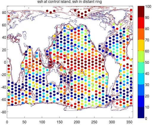
The coherence (or lack of it) between island and off-shore sea-level may be due to the bathymetry, or simply the distance to the deeper waters. The coherence between the
20
distant sea-level and that at the “control island” displays the same spatial dependence as for the island analysis (Fig. 3). In fact, Fig. 2a could almost be a subsampled version of Fig. 3.
The spatial variability in Fig. 3 is not a function of latitude alone, but also includes some longitude dependence. Regions of high eddy energy, such as the Kuroshio, the
25
OSD
9, 3049–3070, 2012Island and ocean sea-level
J. Williams and C. W. Hughes
Title Page
Abstract Introduction
Conclusions References
Tables Figures
◭ ◮
◭ ◮
Back Close
Full Screen / Esc
Printer-friendly Version Interactive Discussion
Discussion
P
a
per
|
Dis
cussion
P
a
per
|
Discussion
P
a
per
|
Discussio
n
P
a
per
|
3.3 Correlation by timescale
To investigate the correlation by timescale in more detail, we calculate the magnitude squared coherence estimate,γxy, using the Matlab function mscohere. This is defined as
γxy(σ)= |Sxy(σ)| 2
Sxx(σ)Syy(σ) ,
5
whereSxy is the cross power spectral density, thusγxy(σ) has values between 0 and 1 and indicates how wellx, the signal at the island, corresponds toy, the signal in deep water, at each frequency (Emery and Thomson, 2001).x andy are chosen fromh,φ
andp.
10
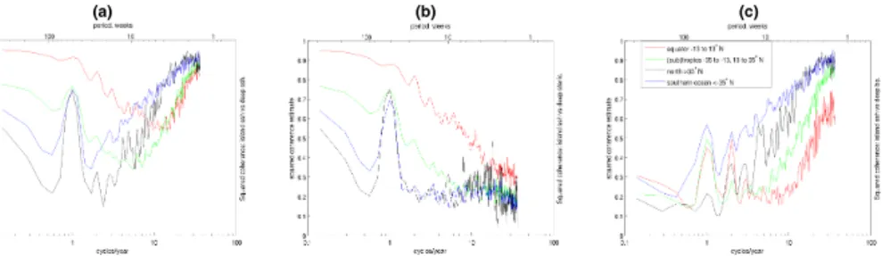
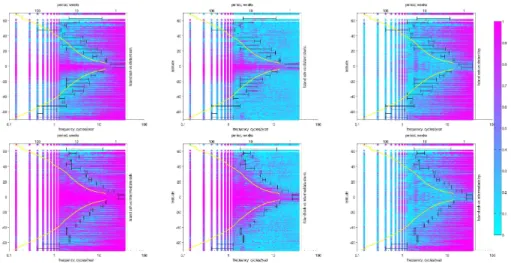
Figure 4 shows γhh, γhφ, γhp, the magnitude squared coherence of sea-surface height at islands and signals in deep water, averaged over four latitude bands. At the annual frequency, there is a sharp peak in γhφ, especially at high latitudes. Other-wise, equatorwards of 35◦ γhφ generally decreases with higher frequencies, and γhp
increases with higher frequencies. γhφ is highest at the equator for all frequencies,
15
and at high frequenciesγhp appears to steadily increase with distance from the equa-tor.γhh≈max(γhφ,γhp), with a dip in coherence at the transition between steric height and bottom pressure, which occurs over periods of between one month and one year according to latitude.
3.4 Correlation by timescale and latitude
20
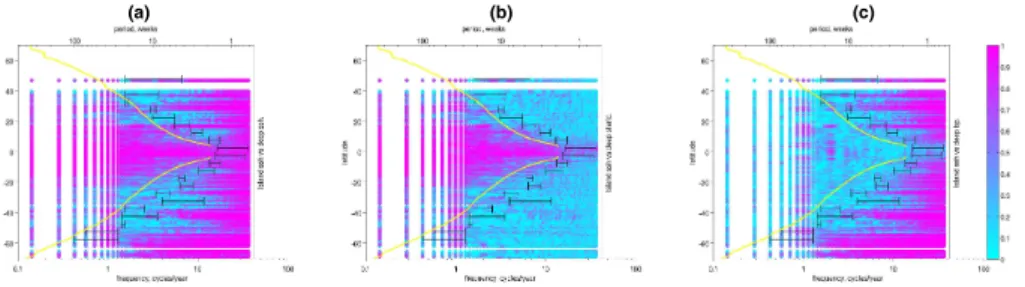
This latitude dependence bears further investigation, and the three panels of Fig. 5 showγhh,γhφ andγhp, respectively, for every island by latitude and frequency. In panel (a) there is a high coherence for low frequencies (left) where the steric part of the offshore signal corresponds well to islandh, and for high frequencies (right) where the bottom pressure part of the offshore signal corresponds well to h, but a zone of low
25
OSD
9, 3049–3070, 2012Island and ocean sea-level
J. Williams and C. W. Hughes
Title Page
Abstract Introduction
Conclusions References
Tables Figures
◭ ◮
◭ ◮
Back Close
Full Screen / Esc
Printer-friendly Version Interactive Discussion
Discussion
P
a
per
|
Dis
cussion
P
a
per
|
Discussion
P
a
per
|
Discussio
n
P
a
per
|
The Rossby frequency, σmax=βR0/4π, is the maximum frequency at which
baro-clinic Rossby waves can exist, based on the linear dispersion relation and the first baroclinic Rossby radius R0, taken from Chelton et al. (1998). The zonal average (in water deeper than 3000 m) Rossby frequency is marked on Fig. 5 as a yellow line and corresponds to periods ranging from about 4 weeks at ±5◦ to longer than a year at
5
high latitudes. Above the maximum Rossby frequency baroclinic Rossby waves are not possible, meaning that the only propagation mechanism for subinertial variability is advective.
Once again,γhh in Fig. 5 panel (a) is close to the larger of γhφ and γhp in panels (b) and (c). The transition region betweenγhφ and γhp is emphasized by black bars.
10
These show, averaged over islands in bands of 5◦latitude, the range between the high-est frequency (shorthigh-est period) for whichγhφ> γhpand the lowest frequency (longest period) for whichγhφ< γhp. All of these bars are to the right of the yellow line, thus at all latitudes, the islandh is explained more by off-shore φ than off-shore p for all frequencies lower than the Rossby wave frequency.
15
All this may lead one to think that at higher frequencies thehsignal offshore is
dom-inated by the p component. However, although the p component certainly becomes
more significant, it is only at a few latitudes that it overtakesφat periods longer than 10 days (the Nyquist period for this dataset).
These transitions are well to the right of the low-coherence zone in Fig. 5a. So in
20
the low-coherence zone the signal is primarily steric off-shore, but this is not sufficient for off-shoreφto translate into an islandhsignal. Only at timescales long enough for baroclinic Rossby waves does the off-shore steric height correlate well with the island sea-surface height.
Bingham and Hughes (2012) found that although coastal sea level could be
recon-25
OSD
9, 3049–3070, 2012Island and ocean sea-level
J. Williams and C. W. Hughes
Title Page
Abstract Introduction
Conclusions References
Tables Figures
◭ ◮
◭ ◮
Back Close
Full Screen / Esc
Printer-friendly Version Interactive Discussion
Discussion
P
a
per
|
Dis
cussion
P
a
per
|
Discussion
P
a
per
|
Discussio
n
P
a
per
|
the mid-depthφ does much better at explaining the island h, as would be expected as it is likely to be closer to the island. Figure 2d shows the variance of island h ex-plained byhin a ring defined as all points with depth 500–1000 m and closer than 2.5◦ latitude and longitude to the island centre. The latitude dependence still exists, though it is weaker than in Fig. 2a, and most islands between 35◦S and 13◦S have around
5
40–80 % of islandh variance explained by offshore φ (mid-depth ring) compared to 10–50 % (deep ring).
The coherence (or lack of it) between island and off-shore sea-level may be due to the bathymetry, or simply the distance to the deeper waters. To test this further we have defined arbitrarily selected “control islands” as 0.75◦×0.75◦squares of water over
10
3000 m deep and compared sea-level there to the surrounding squares between widths 0.75◦ and 2.5◦ (intermediate ring) and between widths 2.5◦ and 5◦ (distant ring). The timescale for coherence between the distant sea-level and that at the “control island” displays the same latitude relationship as for the on-shore vs off-shore results above (Figs. 3 and 6). The dip in coherence extends to longer timescales for the more distant
15
ring. These results show that the dip in coherence does not result from any dynamics specific to islands.
3.5 Admittance
We have also plotted the admittance or transfer function for the islands and rings as defined above. This is defined by
20
Txy(σ)=Sxy(σ)
Sxx(σ) ,
whereSxy is the cross power spectral density, and is calculated using the Matlab func-tion “tfestimate”. This gives informafunc-tion about the ratios of the signals as well, but in fact admittance looks very similar to coherence. The only exception is at the annual period,
25
OSD
9, 3049–3070, 2012Island and ocean sea-level
J. Williams and C. W. Hughes
Title Page
Abstract Introduction
Conclusions References
Tables Figures
◭ ◮
◭ ◮
Back Close
Full Screen / Esc
Printer-friendly Version Interactive Discussion
Discussion
P
a
per
|
Dis
cussion
P
a
per
|
Discussion
P
a
per
|
Discussio
n
P
a
per
|
3.6 Spectral shape of steric signal
The pattern in Fig. 3 is not purely a function of latitude. Points in the most energetic regions seem to have lowhvariance explained by their neighbouring rings, tending to give lower values in the west of basins than the east.
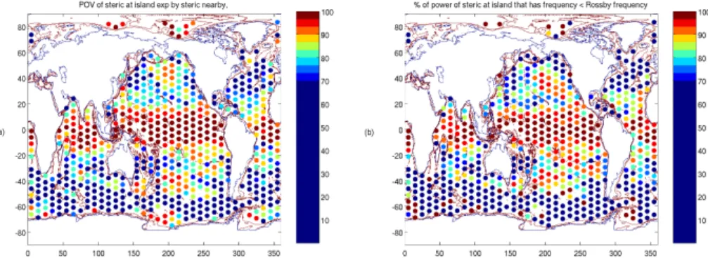
In Fig. 7b we show for each control point the percentage of the steric power spectrum
5
that has frequency lower than the Rossby frequency. If our interpretation is right, then this is the percentage of the variance at each point that occurs in the high coherence spectral band, so should look similar to Fig. 7a, the percentage ofφvariance explained by a 2.5◦ diameter nearby ring.
The spectral shape alone introduces the longitudinal structure of Fig. 7a. A similar
10
plot (not shown) of the percentage of the steric power spectrum that has frequency lower than half the Rossby frequency corresponds almost as well with the percentage of variance of steric explained by steric in a 5◦distant ring. However at this distance, in high-energy regions including the North-West Pacific and Gulf Stream, we find lower coherence in Fig. 7a than this argument predicts. That is, in the regions of high
vari-15
ability, low frequency signals at a distance of around 2◦(∼150 km at mid-latitudes) are not coherent. Eddies matter even at periods longer than a year.
4 Conclusions
Figure 2a showed that the strength of the relationship between island sea level and nearby deep ocean sea level is quite variable, with some latitudes showing rather
20
weakly coupled signals. Decoupling implies that there is either locally-trapped vari-ability associated with the island topography, or that nearby deep ocean signals simply do not propagate to the coast, perhaps because of a topographic barrier to propa-gation. Both of these explanations appear to play a part in the decoupling between deep ocean and coastal continental sea level variability seen by Hughes and Williams
25
OSD
9, 3049–3070, 2012Island and ocean sea-level
J. Williams and C. W. Hughes
Title Page
Abstract Introduction
Conclusions References
Tables Figures
◭ ◮
◭ ◮
Back Close
Full Screen / Esc
Printer-friendly Version Interactive Discussion
Discussion
P
a
per
|
Dis
cussion
P
a
per
|
Discussion
P
a
per
|
Discussio
n
P
a
per
|
decoupling, similar to that seen at islands, also occurs between deep ocean points and surrounding rings. In that sense, island sea level behaves just like sea level at any open ocean point. This suggests that the decoupling must be associated with short wave-length signals which are failing to propagate from a deep ocean ring to its center, and that the topographic barrier is not a dominant factor in this failure.
5
Our spectral coherence analyses (Figs. 4 and 5) support this conclusion. At high frequencies, there is coherence between island and offshore sea level, and this is vir-tually all associated with bottom pressure variability, which typically has large length scales associated with barotropic variability, and dominates the variability out to longer periods at higher latitudes (Vinogradova et al., 2007; Bingham and Hughes, 2008). On
10
moving to lower frequencies, as Fig. 1 shows, steric variability, and therefore baroclinic processes, come to dominate. This results in a dip in coherence, but then a rise again, which always occurs at frequencies lower than (to the left of) the yellow line in Fig. 5, representing the maximum frequency at which linear baroclinic Rossby waves can ex-ist. The Rossby wave dispersion relation is such that, immediately to the left of the
15
yellow line, only a narrow range of wavelengths is permitted. The range of permitted wavelengths expands as frequency decreases, and therefore represents an increasing fraction of the total variability.
Thus, coherent signals appear to be associated with barotropic and wave-like baro-clinic processes. The band of low coherence spreads for some (variable) range to
20
either side of the Rossby wave cut-offfrequency, and appears to represent steric vari-ability which cannot propagate in a wave-like manner. As noted in Hughes and Williams (2010), although much of the actual variability is nonlinear and may be eddy-like, it still often displays many of the features of baroclinic Rossby waves, including westward propagation resulting from a similar mechanism. In this interpretation, poor correlation
25
OSD
9, 3049–3070, 2012Island and ocean sea-level
J. Williams and C. W. Hughes
Title Page
Abstract Introduction
Conclusions References
Tables Figures
◭ ◮
◭ ◮
Back Close
Full Screen / Esc
Printer-friendly Version Interactive Discussion
Discussion
P
a
per
|
Dis
cussion
P
a
per
|
Discussion
P
a
per
|
Discussio
n
P
a
per
|
Other processes will apply to steep and small islands that cannot be resolved by the 1/12 degree model. However it seems unlikely to us that the correlation between island and off-shore sea-level would be increased by such processes, so the pink regions in Figs. 5 and 6 represent the maximum extent of the latitudes and periods for which high coherence can be expected.
5
At high latitudes, linear baroclinic waves propagate so slowly that currents of only a few cm s−1 can be sufficient to overwhelm the wave propagation. In the Antarctic Circumpolar Current, this results in the eastward propagation of all features with wave-lengths shorter than about 300–500 km and a series of stationary, equivalent-barotropic waves at that wavelength (Hughes, 2005; Hughes et al., 1998). This unusual structure
10
is probably responsible for the notably different behaviour seen in the Southern Ocean in Fig. 2.
There appears to be broad agreement between our results and those of Vinogradov and Ponte (2011), although their data is limited to existing gauge locations, so there is a sparser distribution of points, making it harder to see any latitude dependence. The
15
island locations between 20◦N and 20◦S have higher correlation between tide gauges and satellite altimetry than those further north (e.g. Canaries, Azores) and south (e.g. Easter Island, San Felix) (see Fig. 6 in their paper). They used time series of annual means, which would explain the slightly higher correlations than in Fig. 2a – our nearest equivalent figure is percentage of variance of islandhexplained by offshorehfiltered
20
to pass periods>18 months, which looks very similar (Fig. 2c). They also state that “results based on 2 and 3 yr averages do lead to improved agreement between the tide gauge and [altimetry] records”, though with no indication of regional effects.
Vinogradov and Ponte (2011) saw discrepancies between the tide-gauge and altime-try at three islands (San Felix, Juan Fernandez and Easter Island) in the South-Eastern
25
OSD
9, 3049–3070, 2012Island and ocean sea-level
J. Williams and C. W. Hughes
Title Page
Abstract Introduction
Conclusions References
Tables Figures
◭ ◮
◭ ◮
Back Close
Full Screen / Esc
Printer-friendly Version Interactive Discussion
Discussion
P
a
per
|
Dis
cussion
P
a
per
|
Discussion
P
a
per
|
Discussio
n
P
a
per
|
Acknowledgements. Thanks to Rory Bingham for discussions and help with the model diagnos-tics. This work was funded by the UK Natural Environment Research Council, using National Capability funding allocated to the National Centre for Earth Observation and the National Oceanography Centre.
References
5
Bingham, R. J. and Hughes, C. W.: The relationship between sea-level and bottom pres-sure variability in an eddy permitting ocean model, Geophys. Res. Lett., 35, L03602, doi:10.1029/2007GL032662, 2008. 3060
Bingham, R. J. and Hughes, C. W.: Local diagnostics to estimate density-induced sea level variations over topography and along coastlines, J. Geophys. Res.-Oceans, 117, C01013,
10
doi:10.1029/2011JC007276, 2012. 3051, 3057, 3059
Chelton, D., DeSzoeke, R., Schlax, M., El Naggar, K., and Siwertz, N.: Geographical variabil-ity of the first baroclinic Rossby radius of deformation, J. Phys. Oceanogr., 28, 433–460, doi:10.1175/1520-0485(1998)028<0433:GVOTFB>2.0.CO;2, 1998. 3057
Emery, W. J. and Thomson, R. E.: Data Analysis Methods in Physical Oceanography, Elsevier,
15
Amsterdam, 2001. 3056
Hughes, C.: Nonlinear vorticity balance of the Antarctic Circumpolar Current, J. Geophys. Res.-Oceans, 110, C11008, doi:10.1029/2004JC002753, 2005. 3061
Hughes, C. W. and Williams, S. D. P.: The color of sea level: Importance of spatial variations in spectral shape for assessing the significance of trends, J. Geophys. Res.-Oceans, 115,
20
C10048, doi:10.1029/2010JC006102, 2010. 3051, 3054, 3059, 3060
Hughes, C. W., Jones, M. S., and Carnochan, S.: Use of transient features to iden-tify eastward currents in the Southern Ocean, J. Geophys. Res., 103, 2929–2943, doi:10.1029/97JC02442, 1998. 3061
Leuliette, E. W., Nerem, R. S., and Mitchum, G. T.: Calibration of TOPEX/POSEIDON and Jason
25
altimeter data to construct a continuous record of mean sea level change, Marine Geodesy, 27, 79–94, doi:10.1080/01490410490465193, 2004. 3050
simu-OSD
9, 3049–3070, 2012Island and ocean sea-level
J. Williams and C. W. Hughes
Title Page
Abstract Introduction
Conclusions References
Tables Figures
◭ ◮
◭ ◮
Back Close
Full Screen / Esc
Printer-friendly Version Interactive Discussion
Discussion
P
a
per
|
Dis
cussion
P
a
per
|
Discussion
P
a
per
|
Discussio
n
P
a
per
|
lated with eddy-permitting and eddy-resolving ocean models, Ocean Model., 28, 226–239, doi:10.1016/j.ocemod.2009.02.007, 2009. 3052
Vignudelli, S., Kostianoy, A., Cipollini, P., and Benveniste, J. (eds.): Coastal Altimetry, 1st edn., Springer, Berlin, 2011. 3050
Vinogradov, S. V. and Ponte, R. M.: Low-frequency variability in coastal sea level from tide
5
gauges and altimetry, J. Geophys. Res., 116, C07006, doi:10.1029/2011JC007034, 2011. 3050, 3061
Vinogradova, N. T., Ponte, R. M., and Stammer, D.: Relation between sea level and bottom pressure and the vertical dependence of oceanic variability, Geophys. Res. Lett., 34, L03608, doi:10.1029/2006GL028588, 2007. 3060
OSD
9, 3049–3070, 2012Island and ocean sea-level
J. Williams and C. W. Hughes
Title Page
Abstract Introduction
Conclusions References
Tables Figures
◭ ◮
◭ ◮
Back Close
Full Screen / Esc
Printer-friendly Version Interactive Discussion
Discussion
P
a
per
|
Dis
cussion
P
a
per
|
Discussion
P
a
per
|
Discussio
n
P
a
per
|
(a) (b) (c)
Fig. 5. Magnitude squared coherence of sea-surface height at island and (left to right) (a)
OSD
9, 3049–3070, 2012Island and ocean sea-level
J. Williams and C. W. Hughes
Title Page
Abstract Introduction
Conclusions References
Tables Figures
◭ ◮
◭ ◮
Back Close
Full Screen / Esc
Printer-friendly Version Interactive Discussion
Discussion
P
a
per
|
Dis
cussion
P
a
per
|
Discussion
P
a
per
|
Discussio
n
P
a
per
|