A GAUSSIAN PROCESS BASED MULTI-PERSON INTERACTION MODEL

A GAUSSIAN PROCESS BASED MULTI-PERSON INTERACTION MODEL

T. Klinger, F. Rottensteiner, C. Heipke

Institute of Photogrammetry and GeoInformation, Leibniz Universit¨at Hannover, Germany -(klinger, rottensteiner, heipke)@ipi.uni-hannover.de

Commission III, WG III/3

KEY WORDS:Gaussian Processes, Interactions, Online, Pedestrians, Tracking, Video

ABSTRACT:

Online multi-person tracking in image sequences is commonly guided by recursive filters, whose predictive models define the expected positions of future states. When a predictive model deviates too much from the true motion of a pedestrian, which is often the case in crowded scenes due to unpredicted accelerations, the data association is prone to fail. In this paper we propose a novel predictive model on the basis of Gaussian Process Regression. The model takes into account the motion of every tracked pedestrian in the scene and the prediction is executed with respect to the velocities of all interrelated persons. As shown by the experiments, the model is capable of yielding more plausible predictions even in the presence of mutual occlusions or missing measurements. The approach is evaluated on a publicly available benchmark and outperforms other state-of-the-art trackers.

1. INTRODUCTION

Visual pedestrian tracking is one of the most active research top-ics in the fields of image sequence analysis and computer vi-sion. The generated trajectories carry important information for the semantic analysis of scenes and thus are a crucial input to many applications in fields such as autonomous driving, field-robotics and visual surveillance.

Most available systems for tracking use variants of the recursive Bayes Filter such as the Kalman- or the Particle Filter to find a compromise between image-based measurements (i.e., automatic pedestrian detections) and a motion model. Generally, the motion model is a realisation of a first-order Markov chain which consid-ers the expected dynamic behaviour such as constant velocity or smooth motion. In the absence of measurements, e.g. during an occlusion, the trajectory is continued only by the motion model. For longer intervals of occlusions, however, a first-order Markov chain is prone to drift away from the actual target position. This situation often occurs in crowded environments, where mutual occlusions cannot be avoided and pedestrian movements often do not match the assumption of an un-accelerated motion. Some au-thors explain the deviations from a constant-velocity model as an effect of social forces caused by interactions with other members of a scene (Helbing and Moln´ar, 1995). The information gath-ered from other scene members with respect to motion is often referred to as motion context. In the scope of recursive filter-ing, this motion context carries valuable information for tracking and allows to generate more plausible predictions in the absence of measurements. In turn, more realistic predictions lower the risk of tracking errors such as false negative detections and iden-tity switches. Available context-aware approaches to pedestrian tracking often require binary decisions about group membership of individuals, or they constrain the interactions by a Markovian assumption. In either way, possible correlations between pedes-trians that are not related by the model are discarded.

Our approach considers the context between every possible pair of pedestrians without being explicit about their interactions. To this end we propose a new model for the predictive function of a recursive filter that is based on Gaussian Process Regression. In this context, we formulate a new covariance function taking

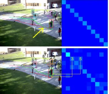
Figure 1. Trajectories generated using a stand-alone Kalman Fil-ter (upper image) and the proposed method (lower image). On the right side of the images the covariance matrices are shown for that scene. The covariance matrix has one row and column for every tracked person in ascending order of their associated iden-tification number. Brighter values indicate higher covariances of the trajectories. Using the stand-alone Kalman Filter, an iden-tity switch occurred after a phase of mutual occlusion (indicated by the arrow), which can be avoided when using the proposed method.

The contributions of this paper are the proposal and comprehen-sive investigation of a new strategy for the incorporation of mo-tion context into a recursive filter. The proposed method is im-plemented in the framework of a recursive tracking-by-detection framework based on (Klinger et al., 2015). A quantitative evalu-ation of the results is carried out on the basis of the Multi Object Tracking Benchmark (Leal-Taix´e et al., 2015).

The remainder of this paper is structured as follows: First we review the related work on the topic of visual multi-pedestrian tracking with a focus on approaches that investigate motion con-text, and on the topic of Gaussian Process Regression applied in the context of tracking (Sec. 2). Then, we investigate Gaussian Process Regression in some more detail. Subsequently, we for-mulate our novel approach (Sec. 3). In the experiments (Sec. 4) we analyse the sensitivity of the proposed method to the varia-tion of the involved parameters and compare the final results with methods from related work on the basis of a publicly available benchmark dataset. In Sec. 5 we conclude our work and give an outlook.

2. RELATED WORK

In this section we briefly review related approaches to context-aware multi-person tracking. We further refer to papers that deal with Gaussian Process Regression in the context of recursive fil-tering approaches.

Motion context. While the main factors for path planning of a pedestrian are well understood (Helbing and Moln´ar, 1995), there are many approaches for embedding this contextual infor-mation into a tracking framework. In (Scovanner and Tappen, 2009) and (Milan et al., 2014) trajectory estimation is formu-lated as an energy minimisation problem, where the energy is the sum of various terms penalising a deviation from an expected behaviour such as collision avoidance, moving towards a prede-fined destination in a straight line and constant velocity. Being aware of other pedestrians’ positions in the scene, such a motion model considers context to avoid collisions, but possible correla-tions of the trajectories that indicate mutual patterns of motion are not further evaluated. Ge et al. (2009), Yamaguchi et al. (2011), Pellegrini et al. (2010), Leal-Taix´e et al. (2011) and Zhang and van der Maaten (2013) incorporate group models which basically have a smoothing effect on the motion of pedestrians of the same group. Although contextual information w.r.t. the motion of in-teracting pedestrians is considered in this way, the binary group membership represented by the model neglects potential correla-tions between subjects from different groups.

Pellegrini et al. (2009), Choi and Savarese (2010), and Yoon et al. (2015) do not apply grouping explicitly. They predict the position of each subject based on the history of all pedestrians. Pellegrini et al. (2009) directly incorporate interactions as well as expected destinations in the scene into the dynamic model of a recursive filter. The degree of interaction between two pedestrians is eval-uated by their current distance and by the angular displacement of their trajectories, i.e., the cosine of the angle between their directions of motion. Choi and Savarese (2010) use a Markov Random Field, where the current state estimate is conditioned on the previous one and undirected edges are established between neighbouring subjects, modelling the social forces caused by in-teractions. However, due to the Markov property interactions of pedestrians which are not direct neighbours in object space are suppressed. As a consequence, potential correlations between subjects that are further apart are neglected. Yoon et al. (2015) also consider the relative motion between subjects by condition-ing the current state estimate on the previous state estimate of the

same subject and on the subjects in its vicinity. In this way, the motion of different interrelated persons is taken into account, but uncertainties about the previous state estimates are not considered in the estimation of the current state estimates.

Gaussian Process Regression. Gaussian Process (GP) Regres-sion models are well studied in the fields of geodesy (where an equivalent to GP Regression is known ascollocation) (Moritz, 1973), geo-statistics (where it is also known askriging), (Krige, 1951), machine learning (Rasmussen, 2006) and computer vision (e.g. Urtasun et al., 2006). We stick to the terminology of ’Gaus-sian Processes’ as our work is set in the context of photogramme-try and computer vision.

A Gaussian Process is a stochastic process in which any finite subset of random variables has a Gaussian joint distribution. Given a set of input points and observed target variables, a pre-diction of the target variable for a test point is made by condi-tioning its target variable on the observed target variables. In this way, the predictive function need not be modelled paramet-rically; it is merely assumed that the input data are correlated. Each conditional distribution over a target variable is Gaussian, which favours their application in the context of recursive Bayes Filters. Ko and Fox (2009) use GPs for Bayesian filtering (GP-Bayes Filter), emphasising that in this way parametric prediction and parametric observation models can be avoided. For the pre-diction of a robot’s state transition, the authors define a Gaus-sian Process taking as input previous state and control sequences of the robot. Ellis et al. (2009) applied GP-Bayes Filters to the tracking of pedestrians, where the input data are trajectories of different persons observed in the past. The problem is formulated as a regression task, where velocities are estimated on the basis of the previously observed trajectories. For a predictive model which is representative for a complete scene, a high amount of training data may be required (depending on the complexity of the scene). As the trajectories are required a priori, the applica-tion is restricted to offline processing. Kim et al. (2011) apply GP based regression for the prediction of motion trajectories of vehicles. Individual trajectories are assigned to clusters and out-liers are detected when the trajectories deviate from a so-called mean flow field. By the explicit association of the trajectories to clusters, possible correlations between trajectories from different clusters are not considered. Later the same authors applied GP re-gression to detect regions of interest for camera orientation, when acquiring images of a football match, by looking at the means of the regression model which reflect the expected destinations of the involved subjects (football players) (Kim et al., 2012). Here, the motion trajectories are not regarded further and persons are correlated based on the spatial distance only. In these works, the input data are the 2D locations of the subjects and the target vari-ables are their velocities.

the similarity between trajectories at runtime. In this way, we di-rectly incorporate contextual information into the tracking frame-work and simultaneously estimate the velocities together with the interactions. This enables more reliable predictions even in the absence of measurements.

3. METHOD

In this section we explain the principles of Gaussian Process Re-gression (GPR) and formulate the prediction model of a recursive filter as a GPR problem. To make the prediction sensitive to inter-actions, we propose a new covariance function, which takes a pair of motion trajectories as input and computes a measure of simi-larity based on the motion direction and the spatial distance of the trajectories. We assume that pedestrians interact to the degree of the covariance of their motion trajectories.

3.1 Gaussian Process Regression

In a Gaussian Process Regression model, it is assumed that the function values of a target variableyare drawn from a noisy pro-cess:

y=f(x) +n

with Gaussian white noisenwith varianceσ2

n. The regression

functionf(x) = t(x) +sis composed of a deterministic part

t(x), also referred to as thetrend, and a stochastic parts ∼ N(0,Σss), which is referred to as thesignaland which follows a

zero-mean normal distribution with covarianceΣss. It is further

assumed that the signal at close positions is correlated. Given a set of observed input and target variables

D={(x1, y1), ...,(xn, yn)}, the aim is to predict the target vari-abley∗for a new input pointx∗. By definition, any finite subset

of the random variables in a GP has a Gaussian joint distribu-tion (Rasmussen, 2006). Hence the joint distribudistribu-tion of an un-known target variabley∗and the observed datay={y1, ..., yn} is Gaussian and can be modelled according to Eq. 1,

y

y∗

∼ N

E(y)

E(y∗)

,

K KT

∗

K∗ K∗∗

(1)

whereE(y)andE(y∗)are the expected values of the observed

and the unknown target variables that correspond to the trend. The covariance matrix is a block matrix, whose elements are specified by a covariance functionk(xi, xj). The matrixK is the covariance matrix of the observed target variables, such that

K(i, j) = k(xi, xj), K∗ is the vector of covariances of the

observed and the unknown target variables, such thatK∗(i) =

k(x∗, xi), andK∗∗ =k(x∗, x∗)is the variance of the unknown

target variable. One of the most prominent realisations of the co-variance function is the squared exponential or Gaussian function (Rasmussen, 2006).

k(xi, xj) =σ2f·exp

−(xi−xj)

2

2l2

+σ2n·δ(i=j) (2)

Eq. 2 describes a Gaussian covariance function, where the co-variance of two input pointsxiandxjis dependent on their pair-wise distance with decreasing covariance at growing distances. The signal varianceσ2

f basically controls the uncertainty of

pre-dictions at input points far from observed data. The characteristic length-scalelcontrols the range of correlations in the input space. In Eq. 2σ2

nis the noise variance accounted for in the diagonal

elements ofK, andδ(i = j) is the Kronecker delta function, which is1fori=jand0otherwise.

The prediction of a new target variable for the input pointx∗is

made by building the conditional distribution of the desired target

variabley∗based on Eq. 1. Since the distribution in Eq. 1 is

Gaussian, the same holds true for the conditional probability of the unknown target variable. In a Gaussian Process Regression model, the distribution over the predicted target variable thus can be written as Eq. 3,

P(y∗|y)∼ N(GPµ(x∗,D),GPΣ(x∗,D)), (3)

with

GPµ(x∗,D) =E(y∗) +K∗K −1

(y−E(y)), (4)

and

GPΣ(x∗,D) =K∗∗−K∗K −1

K∗T. (5)

The estimated valueyˆ∗=GPµ(x∗,D)corresponds to the mean

of Eq. 3, andσˆ2

y∗=GPΣ(x∗,D)is the variance of the estimated

target variable.

3.2 Implicit Motion Context

For the application in a recursive filter, the aim is to formulate a predictive model which takes account of the assumption that pedestrians do not move in a way completely independent from other scene members. Similar to Ellis et al. (2009) and Kim et al. (2011) we model the velocityvias the target variable of a GP Regression model independently for each input dimension. Dif-ferent from the related work we take as input the trajectories and velocities of all currently tracked pedestrians. In accordance with the GPR model we decompose the velocity of a pedestrian into a trend and a signal, and argue that the signal of two pedestrians is correlated in case of interactions. In analogy to Eq. 3 the predic-tive model for the velocity can be written in probabilistic form as a Gaussian distribution over the predicted velocity:

P(vi|v)∼ N(GPµ(Ti,T),GPΣ(Ti,T)), (6)

where the given set of input and target variables T={(T1, v1), ...,(Tn, vn)}consists of the trajectories and cur-rent velocity estimates of allncurrently tracked pedestrians. The predicted velocity of a personican be found using Eqs. 4 and 5. We propose a novel covariance function (Eq. 7) that computes the covariance of two trajectoriesTi = [Xi,t−h, ...,Xi,t]T and Tj = [Xj,t−h, ...,Xj,t]

T

w.r.t. their current andhmost recent positions in object space. We assume that the motion direction and spatial distance of two pedestrians are representative for their interactions. This is why the function takes into account the angu-lar displacement of the motion directions and the spatial distance between the current positions.

k(Ti,Tj) =w(Ti,Tj)σ2

fexp

−(Xi,t−Xj,t)

2

2l2

+σ2

n,iδ(i=j)

(7) The first factor in Eq. 7,w(Ti,Tj), is what we define as the an-gular functionwhich takes into account the angular displacement

αijof two trajectories (see Eq. 8). The noise varianceσ2

n,i

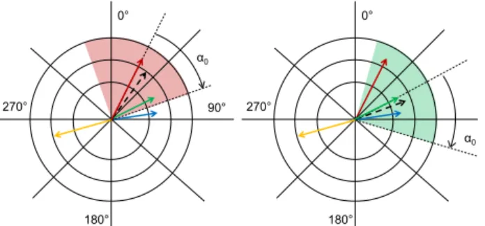
re-flects the uncertainty about the input velocities and is added along the diagonal ofK. We computeαijas the angle between the con-necting lines of the first and last points ofTiandTj, respectively. The function returns the cosine of the angular displacement if the angular displacement is smaller than a thresholdα0, and other-wise it is set to zero.

w(Ti,Tj) =cos(αij)·δ(αij≤α0) (8)

The signal varianceσ2

ar-0°

180° 270°

α0

0°

90°

180° 270°

α0

Figure 2. Angular displacements and weighted average velocities (see text for details).

rows in different colours, and the shaded regions show the ranges of possible correlations for the red (left) and the green (right) instance. These ranges are determined by the angular threshold

α0, and all velocities inside the shaded region contribute to the estimated velocity. For a tracking in 2D, the weighted average velocity vectorv¯iis drawn by the broken arrow in Fig. 2. We

modelv¯ias the trend of the Gaussian Process in accordance with

Eq. 9.

¯

vi=E(vi) =

1

n

X

j=1...n

w(Ti,Tj)·vj (9)

The exponential function on the r.h.s. of Eq. 7 accounts for the spatial distance between the current position estimatesxi,tand

xj,t. Fig. 3 shows velocity estimates computed using the

expo-nential function for all points in a discrete grid of0.5m×0.5m, using the current positions of the persons as input variables and their velocities as observed target variables. The variances of the predicted velocities are indicated by the colours of the arrows, where red indicates high values and green indicates low values. Note that due to the exponential decrease of the covariances the predicted velocities for positions with a low density of observed data have higher variances (depending onσ2

f), and the estimated

velocities in these areas tend to zero. While in Eq. 7 the ex-ponential function causes high covariances for all pedestrians at short pairwise distances (depending onl), the delta function sup-presses correlations of pedestrians moving in different directions (depending on the angular displacement thresholdα0).

Having defined the covariance function in Eq. 7, the covariance is computed for every pair of currently tracked pedestrians. Given the observed input dataT, the predicted values of the velocity componentsˆviand their variancesσˆ2

vi are found in accordance

with Eqs. 4 and 5, respectively:

ˆ

vi= ¯vi+K∗K−

1

(v−E(v)), (10)

ˆ

σvi2 =K∗∗−K∗K −1

K∗T. (11)

3.3 Recursive Bayesian estimation

For the practical application of the proposed model in a recursive filter we use an Extended Kalman Filter model. Generally, a re-cursive Bayesian estimation framework consists of a predictive model for the transition of the state vectorwbetween successive time steps, and a measurement model, which yields a mapping from the state space to the observation space (here: the image). We model a six-dimensional state vector that accounts for the 3D position(X, Y, Z), the heightHand the velocity componentsvX

andvZin the dimensionsXandZparallel to the ground plane, which is assumed to be a plane at a known and constant height below the camera.

Figure 3. Motion vector field with covariances as a function of the distance only. The magnitudes of the velocities are exaggerated by a factor of two for visualisation.

Prediction. One Gaussian Process is defined independently for the velocityvXandvZ,

vXi∼ N(GPµ_X(Ti,T),GPΣ_X(Ti,T)) (12)

and

vZi∼ N(GPµ_Z(Ti,T),GPΣ_Z(Ti,T)), (13)

so that the prediction of the velocities is accomplished by finding the means of the univariate Gaussian distributions in accordance with Eqs. 10 and 11. The predictive model of the recursive filter is a multivariate Gaussian distribution over the state vector, Eq. 14, conditioned on the previous state vectorswt−1,i=1...nand

trajectoriesTi=1...nof allnpedestrians being tracked:

P(w+t,i|wt−1,i=1...n,Ti=1...n) =N(µ

+

w,t,Σ+ww,t), (14)

with mean vectorµ+

w,t:

µ+

w,t= [X

+

t , Y

+

t , Z

+

t , H

+

t , v

+

X,t, v

+

Z,t] T

(15)

and covariance matrixΣ+

ww,t:

Σ+

ww,t= ΨΣww,t−1Ψ

T

+ Σp, (16)

whereΨis the transition matrix that transforms the state vec-tor from the previous time step to the current time step (Rabiner, 1989). We assume zero acceleration in the directions ofXand

Z and zero velocity in vertical direction, i.e., for the parameters

Y andH. Deviation from these assumptions may occur due to unforeseen accelerations (aX,aZ) and velocities (vY,vH). These effects are captured by a zero-mean multivariate normal distri-bution over the vectoru= [aX, vY, aZ, vH]T _{with expectation} E(u) = 0and covarianceΣuu =diag(σ2aX, σ

2

vY, σ

2

aZ, σ

2

vH).

These uncertainties are related to the covariance of the predicted state vector by the process noise Σp = GΣuuGT, where the

matrixGis the Jacobian of the transition matrix. In our case the accelerations are induced by interactions with other pedes-trians, so that the variances computed by the Gaussian Process Regression reflect the uncertainties about the process noise, i.e.,

σ2

aX=GPΣ_X(Ti,T)·∆t−2andσaZ2 =GPΣ_Z(Ti,T)·∆t−2, where∆tis the time difference between two consecutive frames. Note that the noise variancesσ2

n,i, which reflect the uncertainties

about the observed target variables in Eq. 7, are the posterior vari-ances of the velocities from the previous time step. Incorporating the estimated velocities into the predicted state vector yields the following functional model of the prediction:

Position:

X+

t =Xt−1+v +

X,t∆t

Z+

t =Zt−1+v +

Z,t∆t

Height:

Y+

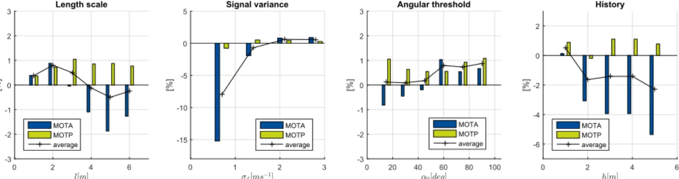
Figure 4. Variation of the parameters and difference of the sum of MOTA and MOTP metrics relative to the results from the stand-alone Kalman Filter.

Ht+=Ht−1

Velocity:

vX,t+ = ˆvX∗

v+Z,t= ˆvZ∗

Update. As in Klinger et al. (2015), we apply a Dynamic Bayesian Network (DBN) which combines the results of a pedes-trian detector, an instance specific classifier with online training capability and a Kalman Filter model in a single probabilistic tracking-by-detection framework. The update step of the recur-sive filter is guided by the collinearity equations. The results of the pedestrian detector and the instance specific classifier are modelled as observations of the positions of the feet and the head of the pedestrians in the image. We apply a pedestrian detec-tor on the basis of the HOG/SVM (Dalal and Triggs, 2005) and an instance specific classifier on the basis of Online Random Forests (Saffari et al., 2009). We further use a fictitious obser-vation for the height of the feet, which is identical to the height of the ground plane. This observation basically enables the conver-sion of 2D image coordinates to 3D world coordinates and, thus, tracking in 3D space.

4. EXPERIMENTS

The covariance function we proposed in Sec. 3. depends on four different parameters: The signal varianceσ2

f, the length-scale l, the angular thresholdα0 and the history of recent trajectory pointsh. For practical application,α0, h, σf andl are learnt from the training data of the 3DMOT benchmark dataset (Leal-Taix´e et al., 2015) using the direct search approach (Hooke and Jeeves, 1961). In a first experiment we demonstrate the sensitiv-ity of the tracking results w.r.t. the mentioned parameters. We furthermore evaluate our approach against methods from related work on the basis of the 3DMOT benchmark.

4.1 Training of the parameters

For the determination of the parametersp={α0, h, σf, l}that yield optimal results on the training data, we take the argument variablespˆthat solve the minimisation problem

ˆ

p= argmin p

1−MOTA(p) +MOTP(p)

2 .

We applied the direct search approach and changed one parame-ter at a time, keeping the others fixed. The parameparame-ters yielding the best results are kept fix during the variation of the next pa-rameter. We assume independence of the parameters and do not further iterate this procedure. As all evaluation metrics used in

the experiments, except for the runtime, essentially depend on p, the notation withpas function argument will be avoided in the remainder of this paper. MOTA and MOTP are the classifi-cation of events, activities, and relationships(CLEAR) metrics Multiple Object Tracking Accuracy and Multiple Object Track-ing Precision as defined by Bernardin and Stiefelhagen (2008). The MOTA metric takes into account false positive (FP) and false negative (FN) assignments as well as identity switches (IDs). The MOTP metric reflects the geometric accuracy of the tracking re-sults. A detection is counted as correct if the estimated position of the feet is not more than one metre apart from the reference. In Fig. 4 the results of the training procedure are visualised. The Figure is divided into four parts, each showing the results achieved by the variation of one parameter. The results are drawn relative to the results achieved bynotusing the proposed method, that is, by using a stand-alone Kalman Filter instead. The curve shows the average gain or loss of MOTA and MOTP achieved by using the proposed method (the connecting lines are just drawn for visual support). The parameters associated to the peaks of the averagecurves are taken as optimal values.

We determined values ofl = 2m,σf = 2m/s,α0 = 90◦and

h = 1mto yield optimal results. The length-scale parameter indicates that interactions take place basically in a radius of2m

around a person. The signal varianceσ2

f controls the maximum

range of velocities and basically limits the velocity estimates far from the input data. The value achieved by the training thus in-dicates that68%of the velocities are expected to lie in a range of±2m/s. The angular threshold of90◦_{indicates that}

consider-ing all persons movconsider-ing with an angular displacement of at most 90◦_{positively affects the tracking results. The history of1m}

in-dicates that only the last metre of the trajectories contributes to the tracking; if longer parts of the trajectories are taken into ac-count, sudden changes in the direction of motion do not reflect instantaneously in the covariances of the trajectories, and the per-formance decreases.

4.2 3DMOT challenge

Here, we report results achieved on the 3DMOT benchmark dataset (Leal-Taix´e et al., 2015) using our approach. For the ini-tialisation of new trajectories we only use the automatic detection results provided along with the benchmark dataset. Our results and results from Pellegrini et al. (2009), Leal-Taix´e et al. (2011), Klinger et al. (2015) and from a baseline tracker are available online1_{. The test dataset consists of two image sequences, the}

PETS09-S2L2 sequence from a campus and the AVG-TownCentre from a pedestrian zone. The average evaluation metrics achieved on the test sequences are given in Table 1, where they are com-pared to the related work (as of Dec. 2015). The reported met-rics include the false alarms per frame (FAF), the ratio of mostly

Method Avg. Rank MOTA MOTP FAF MT ML FP FN IDs Frag. Hz

GPDBN (ours) 2.4 50.2 62.0 2.5 26.5% 18.7% 2252 5842 267 347 0.1

Klinger et al. (2015) 2.0 51.1 61.0 2.3 28.7% 17.9% 2077 5746 380 418 0.1

Leal-Taix´e et al. (2011) 3.1 35.9 54.0 2.3 13.8% 21.6% 2031 8206 520 601 8.4

Baseline 3.6 35.9 53.3 4.0 20.9% 16.4% 3588 6593 580 659 83.5

Pellegrini et al. (2009) 3.9 25.0 53.6 3.6 6.7% 14.6% 3161 7599 1838 1686 30.6

Table 1. 3D MOT 2015 results

tracked (MT, a person is MT if tracked for at least80%of the time being present in consecutive images) and mostly lost (ML, if tracked for at most20%) objects, the numbers of false positive and false negative detections, the number of identity switches, the number of interruptions during the tracking of a person (Frag.), the processing frequency (Hz, in frames per second) as well as MOTA and MOTP. The average rank shows the mean of the ranks achieved in the individual metrics.

As shown in Tab. 1, our method yields the best results in terms of geometric accuracy (MOTP), identity switches and interrup-tions, and an overall second best average rank of2.4. Compared to the method of Klinger et al. (2015), on which our method is constructed, the results show that we have about8%more false positive and2% more false negative assignments. It is worth noting that although approximately the same rate of pedestrians could be tracked throughout their existence in the image sequence (as measured by the MT score), both the number of ID switches and interruptions could be reduced clearly about30%and16% compared to the work of Klinger et al. (2015), who do not take interactions into account. The benefit of using the implicit mo-tion context as proposed in this paper can be attributed to the improved predictive model of the underlying recursive filter, in which the information of every tracked pedestrian is considered. In this way, even in the absence of observations a trajectory can be continued by exploiting the information about correlated (in-teracting) pedestrians. In such a case, a trajectory is only con-tinued based on the predictions. As in a recursive filter the prior information (i.e., the previous state estimate) typically defines the search space for new target positions, an improved motion model yields fewer interruptions of trajectories. If motion context is not considered in the motion model, the prediction is prone to drift away from the target while at the same time being susceptible to an assignment to another target (causing an identity switch). Such a situation occurred in the exemplary scene depicted in Fig. 1 at the beginning of the paper.

The MOTP shows the normalised distance of a correct detection from the reference annotation in metres. According to that met-ric, the results of our method yield the highest geometric preci-sion currently reported on the 3DMOT Benchmark (see Tab. 1, as of Dec. 2015). The MOTP value of62.0indicates that the average positional displacement of the automatically estimated pedestrian positions is about38cm. This average offset basically stems from uncertainties at the conversion of the monocular im-age coordinates to the ground plane, which is assumed to be hor-izontal. Although the difference between the best (this) and the second best method in terms of that metric is only small, it shows that the covariance structure of pedestrians carries valuable in-formation for the determination of the pedestrians’ motion, and thus of the pedestrians’ position. W.r.t. to processing time, this method, which is based on the same framework as Klinger et al. (2015), performs worst among the competing methods with only 0.1frames per second. The prediction using the Gaussian Pro-cess Regression is as complex as the inversion of an×nmatrix (i.e.,O(n3

)), wherenis the number of pedestrians and only in the range of ten to thirty in our application scenario. Thus, the processing time of the algorithm is very similar to that of Klinger

et al. (2015), where most of the computation time is used for the training of and classification with the online random forest clas-sifier.

5. CONCLUSIONS

In this paper, we propose a new predictive model for a recursive Bayesian filter on the basis of Gaussian Process Regression. Us-ing the proposed method, the state vector of a pedestrian is pre-dicted from the states of all pedestrians being tracked. In this con-text, we propose a new covariance function which computes the covariance of two motion trajectories in terms of motion direction and spatial distance. The method is applied to a public benchmark dataset and the results show that the number of identity switches, the number of interruptions, and the geometric accuracy could be improved in comparison to the state-of-the-art. However, our tracking results also reveal an increase of false positive assign-ments, which are due to mismatches between the expected and the true motions. Such cases often occur during an occlusion, so that the trajectories are continued towards spurious destinations, causing false positive detections. To remedy such effects, a multi-modal state representation will be investigated to evaluate both a prediction with and without using contextual information at the same time. When new measurements are obtained, the trajectory will be continued using the prediction that better coincides with the measurements.

REFERENCES

Bernardin, K. and Stiefelhagen, R., 2008. Evaluating multiple object tracking performance: the CLEAR MOT metrics. Journal on Image and Video Processing, vol. 2008, no. 1, pp. 1–10.

Choi, W. and Savarese, S., 2010. Multiple target tracking in world coordinate with single, minimally calibrated camera. In: Proc. European Conference on Computer Vision (ECCV), Springer, pp. 553–567.

Dalal, N. and Triggs, B., 2005. Histograms of oriented gradients for human detection. In: Proc. IEEE Conference on Computer Vision and Pattern Recognition (CVPR), pp. 886–893.

Ellis, D., Sommerlade, E. and Reid, I., 2009. Modelling pedes-trian trajectory patterns with gaussian processes. In: Proc. IEEE International Conference on Computer Vision (ICCV) Workshop, pp. 1229–1234.

Ge, W., Collins, R. T. and Ruback, B., 2009. Automatically de-tecting the small group structure of a crowd. In: Proc. IEEE Workshop on Applications of Computer Vision (WACV), pp. 1– 8.

Helbing, D. and Moln´ar, P., 1995. Social force model for pedes-trian dynamics. Physical review. E, Statistical Physics, Plasmas, Fluids, and Related Interdisciplinary Topics, 51 (5) pp. 4282– 4286.

Kim, K., Lee, D. and Essa, I., 2011. Gaussian process regression flow for analysis of motion trajectories. In: Proc. IEEE Interna-tional Conference on Computer Vision (ICCV), pp. 1164–1171.

Kim, K., Lee, D. and Essa, I., 2012. Detecting regions of interest in dynamic scenes with camera motions. In: Proc. IEEE Con-ference on Computer Vision and Pattern Recognition (CVPR), pp. 1258–1265.

Klinger, T., Rottensteiner, F. and Heipke, C., 2015. Probabilistic multi-person tracking using dynamic Bayes networks. In: ISPRS Annals of the Photogrammetry, Remote Sensing and Spatial In-formation Sciences, Volume II-3/W5, pp. 435-442.

Ko, J. and Fox, D., 2009. GP-BayesFilters: Bayesian filtering using Gaussian process prediction and observation models. Au-tonomous Robots 27(1), pp. 75–90.

Krige, D. G., 1951. A statistical approach to some basic mine valuation problems on the Witwatersrand. Journal of Chemical, Metallurgical, and Mining Society of South Africa 94(3), pp. 95– 112.

Leal-Taix´e, L., Milan, A., Reid, I., Roth, S. and Schindler, K., 2015. MOTChallenge 2015: Towards a benchmark for multi-target tracking. arXiv:1504.01942 [cs].

Leal-Taix´e, L., Pons-Moll, G. and Rosenhahn, B., 2011. Every-body needs someEvery-body: Modeling social and grouping behavior on a linear programming multiple people tracker. In: Proc. IEEE International Conference on Computer Vision (ICCV) Workshop, pp. 120–127.

Milan, A., Roth, S. and Schindler, K., 2014. Continuous en-ergy minimization for multi-target tracking. IEEE Transactions on Pattern Analysis and Machine Intelligence, 36 (1) pp. 58–72.

Moritz, H., 1973. Least-Squares Collocation. German Geodetic Commission (DGK), Series A, Nr. 75, Munich, Germany.

Pellegrini, S., Ess, A. and Van Gool, L., 2010. Improving data association by joint modeling of pedestrian trajectories and groupings. In: Proc. European Conference on Computer Vision (ECCV), Springer, pp. 452–465.

Pellegrini, S., Ess, A., Schindler, K. and Van Gool, L., 2009. You’ll never walk alone: Modeling social behavior for multi-target tracking. In: Proc. IEEE International Conference on Com-puter Vision (ICCV), pp. 261–268.

Rabiner, L. R., 1989. A tutorial on hidden Markov models and selected applications in speech recognition. Proceedings of the IEEE, 77 (2) pp. 257–286.

Rasmussen, C. E., 2006. Gaussian processes for machine learn-ing. The MIT press.

Saffari, A., Leistner, C., Santner, J., Godec, M. and Bischof, H., 2009. On-line random forests. In: Proc. IEEE International Con-ference on Computer Vision (ICCV) Workshop, pp. 1393–1400.

Scovanner, P. and Tappen, M. F., 2009. Learning pedestrian dy-namics from the real world. In: Proc. IEEE International Confer-ence on Computer Vision (ICCV), pp. 381–388.

Urtasun, R., Fleet, D. J. and Fua, P., 2006. 3D people tracking with Gaussian process dynamical models. In: Proc. IEEE Con-ference on Computer Vision and Pattern Recognition (CVPR), Vol. 1, IEEE, pp. 238–245.

Yamaguchi, K., Berg, A. C., Ortiz, L. E. and Berg, T. L., 2011. Who are you with and where are you going? In: Proc. IEEE Con-ference on Computer Vision and Pattern Recognition (CVPR), pp. 1345–1352.

Yoon, J. H., Yang, M.-H., Lim, J. and Yoon, K.-J., 2015. Bayesian multi-object tracking using motion context from multiple objects. In: Proc. IEEE Winter Conference on Applications of Computer Vision (WACV), pp. 33–40.