Recent transient tracer distributions in the Fram Strait: estimation of anthropogenic carbon content and transport

(1)

OSD

12, 2189–2229, 2015

Cant in the Fram Strait

T. Stöven et al.

Title Page

Abstract Introduction

Conclusions References

Tables Figures

◭ ◮

Back Close

Full Screen / Esc

Printer-friendly Version Interactive Discussion

Discussion

P

a

per

|

Discussion

P

a

per

|

Discussion

P

a

per

|

Discussion

P

a

per

|

Ocean Sci. Discuss., 12, 2189–2229, 2015 www.ocean-sci-discuss.net/12/2189/2015/ doi:10.5194/osd-12-2189-2015

This discussion paper is/has been under review for the journal Ocean Science (OS). Please refer to the corresponding final paper in OS if available.

Recent transient tracer distributions in

the Fram Strait: estimation of

anthropogenic carbon content and

transport

T. Stöven1, T. Tanhua1, M. Hoppema2, and W.-J. von Appen2

1

Helmholtz Centre for Ocean Research Kiel, GEOMAR, Germany

2

Alfred Wegener Institute Helmholtz Centre for Polar and Marine Research, Bremerhaven, Germany

Received: 5 August 2015 – Accepted: 24 August 2015 – Published: 24 September 2015

Correspondence to: T. Stöven (tstoeven@geomar.de)

(2)

OSD

12, 2189–2229, 2015

T. Stöven et al.

Title Page

Tables Figures

◭ ◮

Back Close

Full Screen / Esc

Discussion

P

a

per

|

Discussion

P

a

per

|

Discussion

P

a

per

|

Discussion

P

a

per

|

Abstract

The storage of anthropogenic carbon in the ocean’s interior is an important process which modulates the increasing carbon dioxide concentrations in the atmosphere. The polar regions are expected to be net sinks for anthropogenic carbon. Transport

esti-mates of dissolved inorganic carbon and the anthropogenic off_{set can thus provide}

5

information about the magnitude of the corresponding storage processes.

Here we present a transient tracer, dissolved inorganic carbon (DIC) and total

al-kalinity (TA) data set along 78◦50′N sampled in the Fram Strait in 2012. A theory on

tracer relationships is introduced which allows for an application of the Inverse Gaus-sian - Transit Time Distribution (IG-TTD) at high latitudes and the estimation of an-10

thropogenic carbon concentrations. Current velocity measurements along the same section were used to estimate the net flux of DIC and anthropogenic carbon through the Fram Strait.

The new theory explains the diff_{erences between the theoretical (IG-TTD based)}

tracer age relationship and the specific tracer age relationship of the field data by sat-15

uration eff_{ects during water mass formation and/or the deliberate release experiment}

of SF6in the Greenland Sea in 1996 rather than by different mixing or ventilation

pro-cesses. Based on this assumption, a maximum SF6 excess of 0.5–0.8 fmol kg

−1

was determined in the Fram Strait at intermediate depths (500–1600 m). The anthropogenic

carbon concentrations are 50–55 µmol kg−1in the Atlantic Water/Recirculating Atlantic

20

Water, 40–45 µmol kg−1in the Polar Surface Water/warm Polar Surface Water and

be-tween 10–35 µmol kg−1 in the deeper water layers, with lowest concentrations in the

bottom layer. The net DIC and anthropogenic carbon fluxes through the Fram Strait in-dicate a balanced exchange between the Arctic Ocean and the North Atlantic, although with high uncertainties.

(3)

OSD

12, 2189–2229, 2015

T. Stöven et al.

Title Page

Tables Figures

◭ ◮

Back Close

Full Screen / Esc

Discussion

P

a

per

|

Discussion

P

a

per

|

Discussion

P

a

per

|

Discussion

P

a

per

|

1 Introduction

Changes in the Arctic during the last decades stand in mutual relationship with changes in the adjacent ocean areas such as the Nordic Seas, the Atlantic and the Pacific Ocean. The elevated heat flux of warm Atlantic Water into the Arctic Ocean has, for example, significant influence on the perennial sea ice thickness and volume and thus 5

on the fresh water input (Polyakov et al., 2005; Stroeve et al., 2008; Kwok et al., 2009; Kurtz et al., 2011). The exchange and transport of heat, salt and fresh water through the major gateways like Fram Strait, Barents Sea Opening, Canadian Archipelago and Bering Strait are also directly connected to changes in ventilation of the adja-cent ocean areas (Wadley and Bigg, 2002; Vellinga et al., 2008; Rudels et al., 2012). 10

The ventilation processes of the Arctic Ocean have a major impact on the anthro-pogenic carbon storage in the world ocean (Tanhua et al., 2008). Studying the fluxes of anthropogenic carbon through the major gateways contributes to the estimate of the integrated magnitude of such ocean–atmosphere interactions. It additionally provides information of a changing environment in the Arctic Mediterranean. The required flux 15

data of the prevailing water masses, i.e. current velocity fields, are obtained by time

se-ries of long-term maintained mooring arrays in the diff_{erent gateways. The Fram Strait}

is the deepest gateway to the Arctic Ocean with highest volume fluxes equatorwards and polewards. One of the well-established cross-section mooring arrays is located at

≈78◦50′N in the Fram Strait (Fahrbach et al., 2001; Schauer et al., 2008) which

pro-20

vided the basis for heat transport estimates in the past (Fahrbach et al., 2001; Schauer et al., 2004, 2008; Beszczynska-Möller et al., 2012). However, the current data inter-pretation and analysis of this mooring array is complicated due to a recirculation pattern and mesoscale eddy structures in this area (Schauer and Beszczynska-Möller, 2009; Rudels et al., 2008; Marnela et al., 2013; de Steur et al., 2014). The spatial and tempo-25

ral volume flux variability and the insuffi_{cient instrument coverage in the deeper water}

(4)

OSD

12, 2189–2229, 2015

T. Stöven et al.

Title Page

Tables Figures

◭ ◮

Back Close

Full Screen / Esc

Discussion

P

a

per

|

Discussion

P

a

per

|

Discussion

P

a

per

|

Discussion

P

a

per

|

most relevant but also the most challenging gateway with respect to transport budgets in the Arctic Mediterranean.

Estimating an anthropogenic carbon budget presupposes the knowledge of the con-centration ratio between the natural dissolved inorganic carbon (DIC) and the

anthro-pogenic part (C_ant) in the water column. An estimate of DIC transport across the Arctic

5

Ocean boundaries is provided by MacGilchrist et al. (2014) who used velocity fields by Tsubouchi et al. (2012) and available DIC data. That work provides a proper estimate of DIC fluxes, although it does not separate the specfic share of anthropogenic car-bon and the uncertainties are relatively high. Here we present anthropogenic carcar-bon

column inventories in Fram Strait using a new data set of SF6 and CFC-12 along the

10

cross-section of the mooring array at 78◦50′N and a short meridional section along the

fast ice edge in 2012. The anthropogenic carbon column inventories were estimated using the transient tracers and the Inverse Gaussian transit time distribution (IG-TTD) model. Flux estimates of DIC and anthropogenic carbon with the Atlantic Water, Recir-culating/Return Atlantic Water and Polar Water water masses through Fram Strait are 15

provided based on current velocities measured with moorings. Common error sources and specific aspects using these tracers and method in Fram Strait are highlighted.

2 Material and methods

2.1 Tracer and carbon data

A data set of CFC-12, SF₆, DIC and TA was obtained during the ARK-XXVII/1

expe-20

dition from 14 June to 15 July 2012 from Bremerhaven, Germany to Longyearbyen,

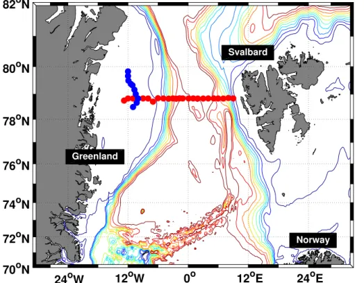
Svalbard on the German research vesselPolarstern(Beszczynska-Möller, 2013).

Fig-ure 1 shows the stations of the zonal section along 78◦50′N, where measurements of

CFC-12, SF6, DIC, and TA were conducted. The meridional section along the fast ice

edge was only sampled for CFC-12 and SF6.

(5)

OSD

12, 2189–2229, 2015

T. Stöven et al.

Title Page

Tables Figures

◭ ◮

Back Close

Full Screen / Esc

Discussion

P

a

per

|

Discussion

P

a

per

|

Discussion

P

a

per

|

Discussion

P

a

per

|

Water samples of the transient tracers CFC-12 and SF₆ were taken with 250 mL

glass syringes and directly measured on board, using a purge and trap GC-ECD sys-tem similar to Law et al. (1994) and Bullister and Wisegarver (2008). The measurement system is identical to the “PT3” system described in Stöven and Tanhua (2014) except

the cooling system and column composition. The trap consisted of a 1/16′′ column

5

packed with 70 cm Heysep D and cooled to −70◦C during the purge process using

a Dewar filled with a thin layer of liquid nitrogen. The 1/8′′precolumn was packed with

30 cmPorasil Cand 60 cm Molsieve 5 Åand the 1/8′′ main column with 180 cm

Car-bograph 1AC. Due to malfunctioning of the Electron Capture Detector (ECD) of the measurement system, the samples of 6 stations (between station 15 and 53) were 10

taken with 300 mL glass ampules and flame sealed for later onshore measurements at GEOMAR. The onshore measurement procedure is described in Stöven and Tanhua

(2014). The precision for the onshore measurements is±4.4 %/0.09 fmol kg−1 for SF₆

and ±1.9 %/0.09 pmol kg−1 for CFC-12. The precision for onboard measurements is

±0.5 %/0.02 fmol kg−1for SF6and±0.6 %/0.02 pmol kg

−1

for CFC-12. 15

The DIC and total alkalinity (TA) samples were taken with 500 mL glass bottles and poisened with 100 µL of a saturated mercuric chloride solution to prevent biological activities during storage time. The sampling procedure was carried out according to Dickson et al. (2007). The measurements of DIC and TA were performed onshore at the GEOMAR, using a coulometric measurement system (SOMMA) for DIC (Johnson 20

et al., 1993, 1998) and a potentiometric titration (VINDTA) for TA (Mintrop et al., 2000).

The precision is±0.05 %/1.1 µmol kg−1for DIC and±0.08 %/1.7 µmol kg−1for TA. The

data of all obtained chemical parameters will be avaiable at CDIAC by the end of 2015. The physical oceanographic data (temperature, salinity, and pressure) from the cruise where the tracers were measured can be found at Beszcynska-Möller and Wisotzki 25

(6)

OSD

12, 2189–2229, 2015

T. Stöven et al.

Title Page

Tables Figures

◭ ◮

Back Close

Full Screen / Esc

Discussion

P

a

per

|

Discussion

P

a

per

|

Discussion

P

a

per

|

Discussion

P

a

per

|

2.2 Water transport data

An array of moorings across the deep Fram Strait from 9◦E to 7◦W has been

main-tained since 1997 by the Alfred Wegener Institute and the Norwegian Polar Institute.

Since 2002, it has contained 17 moorings at 78◦50′N. Here we use the gridded data

from the array from summer 2002 to summer 2010 as described in Beszczynska-Möller 5

et al. (2012). The more recent data has either not been recovered yet or the process-ing is still in progress. The moorprocess-ings contained temperature and velocity sensors at five standard depths: 75, 250, 750, 1500, and 10 m above the bottom. These hourly mea-surements were averaged to monthly values and then gridded onto a regular 5 m verti-cal by 1000 m horizontal grid using optimal interpolation. Since interannual trends are 10

small (Beszczynska-Möller et al., 2012), we consider the long term average volume flux of the following water masses: Atlantic Water advected in the West Spitsbergen

Cur-rent defined as longitude≥5◦E and depth≤750 m; Recirculating and Return Atlantic

Water which is both due to the recirculation of Atlantic Water in Fram Strait (de Steur et al., 2014) and the long loop of Atlantic Water through the Arctic Ocean (Karcher 15

et al., 2012), defined as longitude≤5◦E, mean temperature≥1◦C, and depth≤750 m;

and finally Polar Water flowing southward in the East Greenland Current defined as

mean temperature≤1◦C and depth≤750 m. The estimate of the volume transport

across Fram Strait below 750 m from the moorings is more complicated. The method of Beszczynska-Möller et al. (2012) which was developed to study the fluxes in the West 20

Spitsbergen Current predicts a net southward transport of 3.2 Sv below 750 m. This is unrealistic given that there are no connections between the Nordic Seas and the Arctic Ocean below the sill depth of the Greenland–Scotland Ridge (750 m) other than Fram Strait. No vertical displacements of isopycnals in these two basins are observed that would suggest a non-zero net transport across Fram Strait below 750 m (von Appen 25

(7)

OSD

12, 2189–2229, 2015

T. Stöven et al.

Title Page

Tables Figures

◭ ◮

Back Close

Full Screen / Esc

Discussion

P

a

per

|

Discussion

P

a

per

|

Discussion

P

a

per

|

Discussion

P

a

per

|

2.3 TTD method

A transit time distribution (TTD) model (Eq. 1) describes the propagation of a boundary condition into the interior of the ocean and is based on the Green’s function (Hall and Plumb, 1994).

c(ts,r)=

∞

Z

0

c0(ts−t)e

−λt_·_G₍_t_,_r_)d_t ₍₁₎

5

Here,c(t_s,r) is the specific tracer concentration at yeart_sand locationr,c₀(t_s−t) the

boundary condition described by the tracer concentration at source yearts−tandG(t)

the Green’s function of the age spectratof the tracer. The exponential term corrects for

the decay rate of radioactive transient tracers. Eq. (2) provides a possible solution of the

TTD model, based on a steady and one-dimensional advective velocity and diff_usion

10

gradient (Waugh et al., 2003).

G(t)=

s

Γ3

4π∆2_t3·exp

−Γ(t−Γ)2

4∆2_t

!

(2)

It is known as the Inverse-Gaussian transit time distribution (IG-TTD) whereG(t) is

defined by the width of the distribution (∆_{), the mean age (}Γ_{) and the age spectra of the}

tracer (t). One can define a∆_/Γ _{ratio of the IG-TTD which represents the proportion}

15

between the advective and diff_{usive properties of the mixing processes as included in}

the TTD. The lower the∆_/Γ_{ratio, the higher is the advective share. A}∆_/Γ_{ratio of 1.0}

is the commonly applied ratio at several tracer surveys (e.g. Waugh et al., 2004, 2006; Tanhua et al., 2008; Schneider et al., 2010, 2014; Huhn et al., 2013). Here we also applied this unity ratio to the ARK-XXVII/1 data set.

20

(8)

OSD

12, 2189–2229, 2015

T. Stöven et al.

Title Page

Tables Figures

◭ ◮

Back Close

Full Screen / Esc

Discussion

P

a

per

|

Discussion

P

a

per

|

Discussion

P

a

per

|

Discussion

P

a

per

|

(CFC-12) data above the atmospheric concentration limit of 528 ppt in 2012 (Bullister, 2015) have no clear time information and are thus not applicable.

2.4 Anthropogenic carbon and the TTD

The IG-TTD model can be used to estimate the total amount of anthropogenic carbon in the water column (Waugh et al., 2004). For this purpose it is assumed that the 5

anthropogenic carbon behaves like an inert passive tracer, i.e. similar to a transient tracer. Then applying Eq. (1), the concentration of anthropogenic carbon in the interior

ocean (Cant(ts)) is given by Eq. (3).

Cant(ts)= 0

Z

∞

Cant,0(ts−t)·G(r,t)dt (3)

Cant,0 is the boundary condition of anthropogenic carbon at yearts−t and G(r,t) the

10

distribution function (see Eq. 1). The historic boundary conditions are described by the

diff_{erences between the preindustrial and modern DIC concentrations at the ocean}

sur-face. These anthropogenic off_{sets can be calculated by applying the modern (elevated)}

partial pressures of CO2and then subtracting the corresponding value of the

preindus-trial partial pressure. In each case, the preformed alkalinity was used as second param-15

eter to determine the specific DIC concentrations (calculated using the Matlab version

of the CO2SYS van Heuven et al., 2011). Here we assumed a constantpCO2,water

sat-uration in the surface. Since exact satsat-urations are not well constrained, we present

sen-sitivity calculations of diff_{erent saturation states/disequilibria (see Sect. 3.6 below). The}

atmospheric history ofpCO2,atmis taken from Tans and Keeling (2015). The preformed

20

alkalinity was determined by using the alkalinity/salinity relationship of MacGilchrist et al. (2014). This relationship is based on surface alkalinity and salinity measurements in Fram Strait which were corrected for sea-ice melt and formation processes.

The time dependent boundary conditions (Cant,0) and Eq. (3) can then be used to

calculate anthropogenic carbon concentrations (Cant(ts)) and the corresponding mean

(9)

OSD

12, 2189–2229, 2015

T. Stöven et al.

Title Page

Tables Figures

◭ ◮

Back Close

Full Screen / Esc

Discussion

P

a

per

|

Discussion

P

a

per

|

Discussion

P

a

per

|

Discussion

P

a

per

|

age. Finally, the mean age of Eq. (3) can be set in relation to the transient tracer based

mean age of the water and allows for back-calculatingCant(ts), i.e. it provides the link

between the tracer concentration and the anthropogenic carbon concentration.

3 Results and discussion

3.1 Water masses in Fram Strait

5

To highlight the diff_{erent transient tracer characteristics we defined the water mass type}

of each sample by using the water mass properties suggested by Rudels et al. (2000, 2005) and the salinity and temperature data of this cruise from Beszcynska-Möller and Wisotzki (2012). Note that this water mass classification is not based on an optimum multiparameter analysis and only serves as an indication for this specific purpose. 10

Water masses of the Arctic Ocean are the Polar Surface Water (PSW) which is the cold and less saline surface and halocline water; the warm Polar Surface Water, defined

by a potential temperature (Θ₎_>_{0, which comprises sea ice melt water due to}

inter-action with warm Atlantic Water; the Arctic Atlantic Water/Return Atlantic Water which derives from sinking Atlantic Water due to cooling in the Arctic Ocean; the deep water 15

masses are upper Polar Deep Water (uPDW), Canadian Basin Deep Water (CBDW) and Eurasian Basin Deep Water (EBDW). Deep water formation, e.g. on the Arctic shelves, usually involves densification from brine rejection. The Eurasian Basin Deep Water mixes with Greenland Sea Deep Water so that this layer corresponds to two sources in the Fram Strait (von Appen et al., 2015, in review).

20

Water masses of the Atlantic Ocean/Nordic Seas are the warm and saline Atlantic Water (AW) and the corresponding Recirculating Atlantic Water (RAW); the Arctic In-termediate Water which is mainly formed in the Greenland Sea; the Nordic Seas Deep Water which comprises Greenland Sea Deep Water (GSDW), Iceland Sea Deep Water (ISDW) and Norwegian Sea Deep Water (NSDW) and is formed by deep convection 25

(10)

OSD

12, 2189–2229, 2015

T. Stöven et al.

Title Page

Tables Figures

◭ ◮

Back Close

Full Screen / Esc

Discussion

P

a

per

|

Discussion

P

a

per

|

Discussion

P

a

per

|

Discussion

P

a

per

|

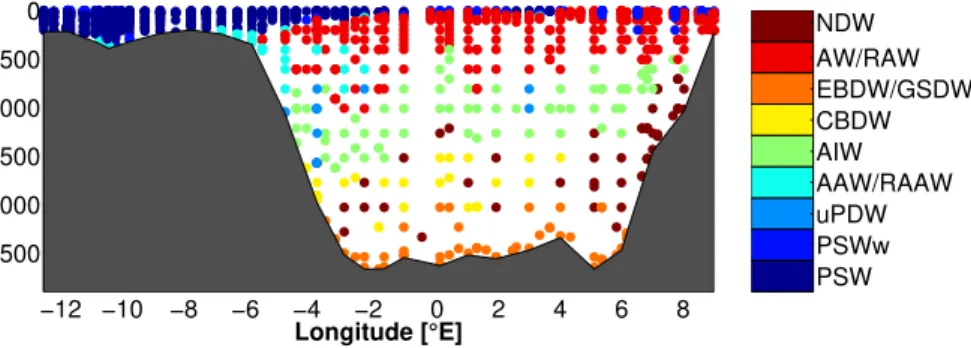
Figure 2 shows the zonal water mass distribution in Fram Strait, which also includes the data from the fast-ice section. The surface layer is dominated by Atlantic Water and Recirculating Atlantic Water in the east and by Polar Surface Water in the west with

a transition between 6◦W and 4◦E where Polar Surface Water overlays the Atlantic

Water. Warm Polar Surface Water can be found within the Atlantic Water between 4– 5

8◦E. The Atlantic Water layer extends down to ≈600 m. Arctic Atlantic Water/Return

Atlantic Water (AAW/RAAW) can be found at the upper continental slope of Greenland between 300–700 m. The intermediate layer between 500–1600 m consists mainly of Arctic Intermediate Water and, at the Greenland slope, partly of Upper Polar Deep

Water. Canadian Basin Deep Water can be found between 1600–2400 m west of 4◦E.

10

Nordic Seas Deep Water is the prevailing water mass along the continental slope of Svalbard between 700–2400 m but can be also observed in the range of the Canadian Basin Deep Water layer. The Eurasian Basin Deep Water/Greenland Sea Deep Water forms the bottom layer below 2400 m.

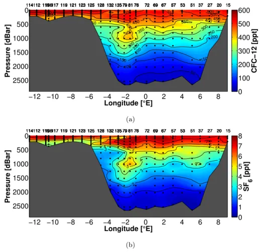
3.2 Transient tracer and DIC distributions

15

Figure 3 shows the partial pressure of CFC-12 and SF6 along the zonal section.

Both tracers have significant concentrations through the entire water column and show a similar distribution pattern. The Atlantic Water shows a relatively homogeneous

dis-tribution of both tracers with CFC-12 partial pressures>450 ppt and SF6 partial

pres-sures>6 ppt. The Polar Surface Water at the shelf region shows a more distinct

struc-20

ture with partial pressures between 4–8 ppt of SF₆ and 410–560 ppt of CFC-12. The

smaller concentration gradient of CFC-12 is related to the recently decreasing atmo-spheric concentration of CFC-12, which causes only slightly varying boundary condi-tions at the air–sea interface (see Sect. 2.3). The high-tracer concentration layer of the Polar Surface Water extends further eastwards as overlaying tongue of the Atlantic 25

Water between 2–6◦W. The intermediate layer between 500–1600 m is characterized

by a clear tracer minimum along the continental slope of Greenland with partial

(11)

OSD

12, 2189–2229, 2015

T. Stöven et al.

Title Page

Tables Figures

◭ ◮

Back Close

Full Screen / Esc

Discussion

P

a

per

|

Discussion

P

a

per

|

Discussion

P

a

per

|

Discussion

P

a

per

|

Arctic Atlantic Water/Return Atlantic Water. East of this minimum, a remarkable tracer

maximum can be observed at 1–3◦W with partial pressures between 3–6 ppt of SF6

and 250–450 ppt of CFC-12. A smaller maximum can be observed between 5–6◦E at

≈1000 m with partial pressures of≈5 ppt of SF₆and≈330 ppt of CFC-12. Both tracer

maxima probably correspond to extensive ventilation events which mainly aff_{ected the}

5

Arctic Intermediate Water and partly the Atlantic Water in the transition zone of both wa-ter masses. The Arctic Inwa-termediate Wawa-ter in the Fram Strait thus consists of recently ventilated areas and less ventilated areas which is also indicated by the large range of transient tracer concentrations. The remaining intermediate layer above 1700 m is

characterized by lower partial pressures between 2–3 ppt of SF₆ and 150–300 ppt of

10

CFC-12 with decreasing concentrations with depth. This gradient extends throughout the deep water layers down to the bottom with partial pressures from 2 ppt down to

0.2 ppt of SF6 and from 150 ppt down to 34 ppt of CFC-12. The fast-ice section is not

presented here since it does not show any diff_{erences compared to the same longitude}

range of the zonal section. 15

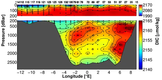
Figure 4 shows the DIC concentrations along the zonal section separated into an

upper and lower panel to highlight the diff_{erent concentration ranges of the}

shal-low and deep water layers. The Greenland shelf region shows concentrations

be-tween 1970 µmol kg−1 in the surface and 2145 µmol kg−1 at ≈200 m. The upper

200 m between 4–8◦E shows increasing concentrations with depth between 2070 and

20

2155 µmol kg−1. There are three significant DIC maxima below 200 m. Two are located

at the continental slope of Svalbard at 300–800 m and at 1400–2100 m with

concen-trations>2158 µmol kg−1 and a maximum concentration of 2167 µmol kg−1. The third

maximum corresponds to the transient tracer maximum at 1–3◦W but extends further

eastwards with concentrations between 2158 and 2162 µmol kg−1. The area of the East

25

Greenland Current at 3–8◦W is characterized by concentrations between 2118 and

2152 µmol kg−1. The deep water below 1700 m shows concentrations between 2150

(12)

OSD

12, 2189–2229, 2015

T. Stöven et al.

Title Page

Tables Figures

◭ ◮

Back Close

Full Screen / Esc

Discussion

P

a

per

|

Discussion

P

a

per

|

Discussion

P

a

per

|

Discussion

P

a

per

|

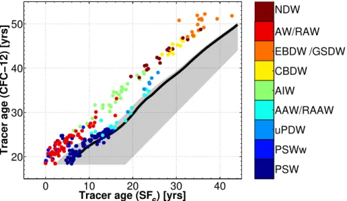
3.3 Transient tracers and the IG-TTD

The IG-TTD can be numerically constrained using transient tracer couples, CFC-12

and SF6in our case, which provides information about the mean age and the

param-eters of the IG-TTD (Waugh et al., 2002; Sonnerup et al., 2013; Stöven and Tanhua, 2014). The method of validity areas, introduced in Stöven et al. (2014), is used to deter-5

mine the applicability of the tracer couple. For this purpose, the tracer age is calculated from the transient tracer concentrations (Waugh et al., 2003) which provides the tracer age relationship of the tracer couple. Figure 5 shows the tracer age relationship of our field data (colored by water mass) in relation to the range of theoretical tracer age

relationships of the IG-TTD, i.e. for ∆_/Γ _{ratios between 0.1–1.8, which describe the}

10

range from advectively dominated to diff_{usively dominated water masses (grey shaded}

area). The black line in Fig. 5 denotes the tracer age relationship based on the unity

ratio of∆_/Γ =_{1.0. Field data which corresponds to this unity ratio would be centered}

around the black line. The Fram Strait data can be separated into two branches of tracer age relationships. The upper branch consists of Atlantic Water/Recirculating At-15

lantic Water, Arctic Intermediate Water, Nordic Seas Deep Water, Eurasian Basin Deep Water/Greenland Sea Deep Water and Canadian Basin Deep Water whereas the lower branch consists of Polar Surface Water, warm Polar Surface Water, Arctic Atlantic Wa-ter/Return Atlantic Water and upper Polar Deep Water. The Polar Surface Water and

warm Polar Surface Water can also partly be found in the upper branch for a SF6tracer

20

age<10 years. Note that the Arctic Atlantic Water/Return Atlantic Water and upper

Po-lar Deep Water show a transition to the upper branch for a SF₆ tracer age larger than

about 20 years. The data shows a more scattered and indistinct structure between 10

and 20 years of the SF6 tracer age. However, the upper branch does not correspond

to the unity ratio and, moreover, it is outside the validity area of the IG-TTD. Water 25

masses related to the lower branch can be applied to the IG-TTD with tendencies

to-wards higher∆_/Γ_{ratios (}_>_{1.0) since the data is clearly above the black line indicating}

(13)

OSD

12, 2189–2229, 2015

T. Stöven et al.

Title Page

Tables Figures

◭ ◮

Back Close

Full Screen / Esc

Discussion

P

a

per

|

Discussion

P

a

per

|

Discussion

P

a

per

|

Discussion

P

a

per

|

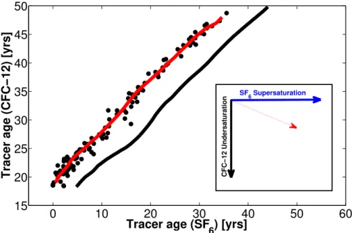
Based on the raw field data, and on assumptions implemented in the IG-TTD (like 100 % saturation of the gases at the surface before entering deeper layers), the IG-TTD

cannot describe the ventilation pattern of the diff_{erent water masses in Fram Strait.}

Nevertheless, by comparing the shape of the two field data branches with the shape of the black line in Fig. 5, it is noted that both branches show similar characteristics 5

as the unity ratio or, generally, as IG-TTD based tracer age relationships. This opens

up the possibility to use the IG-TTD the other way around, i.e. to assume a fixed∆_/Γ

ratio to determine the deviation of transient tracer concentrations rather than using the

transient tracer concentration to determine the ∆_/Γ _{ratio. Since several publications}

found the unity ratio of∆_/Γ =_{1.0 to be valid in large parts of the ocean, we assumed}

10

that this is also true for water masses in Fram Strait. Figure 6 shows the mean tracer age relationship of the upper branch (red line) and the tracer age relationship of the

unity ratio (black line/same as in Fig. 5). The off_{set of the field data related to the}

unity ratio suggests an undersaturation of CFC-12 and/or a supersaturation of SF₆

(see black box in Fig. 6). This uncommon coexistence of under- and supersaturated 15

transient tracers is discussed in the following section.

3.4 Saturations and excess SF6

The surface saturations of transient tracers are influenced by sea surface temperature

and salinity, ice coverage, wind speed, bubble eff_{ects, atmospheric growth rate of the}

tracer and the boundary dwell time of the water parcel (i.e. the time the water parcel is 20

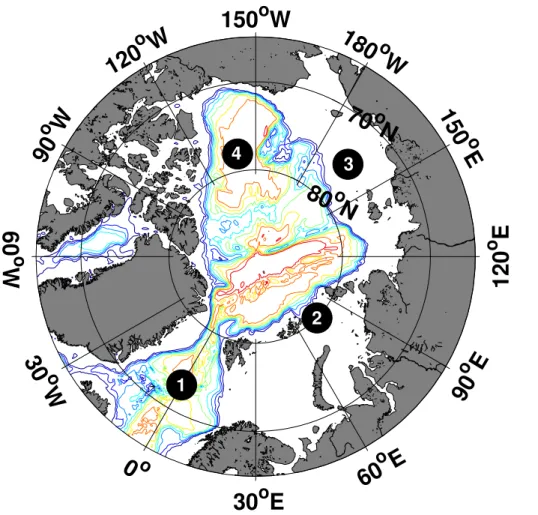
in contact with the atmosphere). However, the saturation state of transient tracers at the air–sea interface before, during and after water mass formation is rarely known, since water mass formation generally occurs in winter at high latitudes, which renders it al-most impossible to obtain measurements. Shao et al. (2013) provide modelled data of

monthly surface saturations of CFC-11, CFC-12 and SF6from 1936 to 2010 on a global

25

scale. This model output can be used to estimate the tracer saturation ratio of diff_erent

water masses by using the surface saturation of the specific formation area and yearly

(14)

OSD

12, 2189–2229, 2015

T. Stöven et al.

Title Page

Tables Figures

◭ ◮

Back Close

Full Screen / Esc

Discussion

P

a

per

|

Discussion

P

a

per

|

Discussion

P

a

per

|

Discussion

P

a

per

|

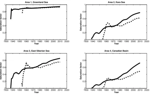
that occur in Fram Strait. The model output shows high variabilities in surface

satura-tions at diff_{erent formation sites, namely the Greenland Sea, the Arctic shelf regions}

and the Arctic open water (Figs. 7 and 8). In contrast, the tracer age relationships of the two branches in Fig. 5 indicate relatively similar deviations in saturation. The complex boundary conditions in the Arctic, e.g. possible gas exchange through ice cover, might 5

bias the results of the saturation model. Therefore, we only used the surface satura-tion of the Greenland Sea (Area 1 in Figs. 7 and 8) which agrees with the findings of Tanhua et al. (2008) who used available field data to investigate historic tracer satu-rations. The IG-TTD based mean age provides the link between the observed tracer concentrations and the corresponding time-dependent saturation factors. Therefore, 10

the saturation factors were applied to the atmospheric history (boundary conditions) of each tracer. These new boundary conditions are then applied to the measured tracer concentrations and the IG-TTD which then yields a saturation-corrected mean age. This mean age in turn can then be used to back-calculate the saturation-corrected tracer concentrations using the originally (uncorrected) boundary conditions. We ex-15

pect that undersaturation eff_{ects also hold for SF}₆_{but are counterbalanced by e}ff_ects

of supersaturation in this survey area.

The SF6 excess is estimated using the corrected CFC-12 concentrations and the

IG-TTD (∆_/Γ =_{1.0) to calculate theoretical SF}₆ _{concentrations of the water parcel,}

i.e. back-calculated SF₆ concentrations. The diff_{erence between the theoretical SF}

6

20

concentration and the measured SF6concentration denotes the SF6excess in the

wa-ter. Note that this SF6 excess is based on the assumption that the IG-TTD and unity

ratio describe the prevailing ventilation pattern of the water masses. Figure 9 shows

the SF6 excess in fmol kg

−1

and ppt for depths below 200 m. This upper depth limit is invoked by the fact that CFC-12 concentrations above the current atmospheric con-25

centration limit cannot be applied to the IG-TTD. The SF₆excess is much higher (0.5–

0.8 fmol kg−1/1.0–1.6 ppt) for northwards propagating water masses compared to water

masses of Arctic origin (0–0.4 fmol kg−1/0–0.8 ppt). There are at least two possible

(15)

OSD

12, 2189–2229, 2015

T. Stöven et al.

Title Page

Tables Figures

◭ ◮

Back Close

Full Screen / Esc

Discussion

P

a

per

|

Discussion

P

a

per

|

Discussion

P

a

per

|

Discussion

P

a

per

|

One possibility refers to the deliberate tracer release experiment in 1996 where

320kg (≈2190 mol) of SF6 were introduced into the central Greenland Sea (Watson

et al., 1999). The patch was redistributed by mixing processes and entered the Arctic Ocean via the Fram Strait and Barents Sea Opening and the North Atlantic via Den-mark Strait and the Faroe Bank Channel (Olsson et al., 2005; Tanhua et al., 2005). 5

Assuming that 50–80 % of the deliberatly released SF6still remains in the Nordic Seas

and the Arctic Ocean (1095–1752 mol) and that 10–50 % of the corresponding total

volume of 1.875×1018–9.375×1018L (Eakins and Sharman, 2010) is aff_{ected, a mean}

off_{set of 0.12–0.93 fmol L}−1 _{is estimated. This mean o}ff_{set is thus in the range of the}

observed SF₆excess concentrations. However, CFC-12 and SF₆data of the Southern

10

Ocean (Stöven et al., 2014) shows similar tracer age relationships compared to the

Fram Strait data but with no influence of deliberately released SF6. This indicates that

probably an additional source of excess SF6exists.

Liang et al. (2013) introduced a model which estimates supersaturations of dissolved

gases by bubble eff_{ects in the ocean. This model predicted an increasing}

supersatu-15

ration for increasing wind speed and decreasing temperature, i.e. the bubble eff_ect

becomes more significant at high latitudes. Furthermore, Liang et al. (2013) show that the magnitude of supersaturation depends on the solubility of the gas. The less sol-uble a gas, the more supersaturation can be expected. Supporting this, Stöven et al.

(2014) describe surface measurements of SF₆ and CFC-12 directly after heavy wind

20

conditions in the Southern Ocean where SF6supersaturations between 20–50 % could

be observed. The CFC-12 concentrations were only aff_{ected to a minor extent which}

indeed seems to be explained by the diff_{erences in solubility. This bubble induced}

su-persaturation can also be expected to apply during the process of water mass forma-tion in the Greenland Sea which usually occurs during late winter, i.e. during a period 25

with low surface temperatures and heavy wind conditions. Furthermore, looking at the

maximum SF6 excess in the Arctic Intermediate Water layer in Fig. 9 and the

gener-ally elevated tracer concentrations of CFC-12 and SF6 in the same area (see Fig. 3)

reaffi_{rms the assumption of bubble induced supersaturation of SF}

(16)

hy-OSD

12, 2189–2229, 2015

T. Stöven et al.

Title Page

Tables Figures

◭ ◮

Back Close

Full Screen / Esc

Discussion

P

a

per

|

Discussion

P

a

per

|

Discussion

P

a

per

|

Discussion

P

a

per

|

pothesis stands in opposition to the current assumption that trace gases are generally undersaturated during water mass formation (Tanhua et al., 2008; Shao et al., 2013).

Future investigations are necessary to determine the diff_{erent impact of under- and}

supersaturation eff_{ects on soluble gases at the air–sea interface. It can be expected}

that possible scenarios are not restricted to distinct saturation states anymore but 5

rather comprise mixtures of equilibrated, under- and supersaturated states of the dif-ferent gases.

3.5 Anthropogenic carbon and mean age

Since CFC-12 is not aff_{ected by tracer release experiments and possibly only to minor}

extent by bubble eff_{ects we used this tracer to calculate the mean age of the water and}

10

the corresponding anthropogenic carbon content. SF6 was only used in the surface

and upper halocline, i.e. where CFC-12 exceeds the atmospheric concentration limit of

528 ppt and where eff_{ects of SF}

6supersaturation are comparatively small.

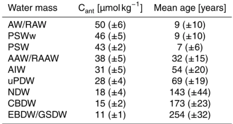
Saturation-corrected tracer data was applied for subsurface data below 100 m whereas surface data was found to be near equilibrium state with the atmosphere. Figure 10 shows the 15

anthropogenic carbon distribution in µmol kg−1and Fig. 11 shows the mean age of the

water masses. According to the relation between transient tracers, mean age and an-thopogenic carbon, the distribution patterns are similar as for the transient tracers. The

highest anthropogenic carbon concentrations of 50–55 µmol kg−1can be found in the

upper 600 m of the Atlantic Water/Recirculating Atlantic Water and a little lower con-20

centrations of 40–45 µmol kg−1 in the Polar Surface Water/warm Polar Surface Water

layer. The mean age of these water masses is between 0–20 years. Note that these water layers show the highest mean current velocities in Fram Strait (see Sect. 3.7

be-low). The area of the tracer maximum at 1–3◦W shows elevated concentrations of 35–

40 µmol kg−1and a mean age of 20–40 years. The remaining water layers below 600 m

25

show anthropogenic carbon concentrations lower than 35 µmol kg−1 with decreasing

concentrations with increasing depth and is comparatively low (<10 µmol kg−1) in deep

(17)

Wa-OSD

12, 2189–2229, 2015

T. Stöven et al.

Title Page

Tables Figures

◭ ◮

Back Close

Full Screen / Esc

Discussion

P

a

per

|

Discussion

P

a

per

|

Discussion

P

a

per

|

Discussion

P

a

per

|

ter/Greenland Sea Deep Water. Accordingly, the mean age increases with increasing depth from 30 to 280 years and shows a maximum mean age of 286 years in the bottom layer at the prime meridian. Table 1 shows the mean values and standard deviation of each specific water layer.

The determined values correspond to the findings of Jutterström and Jeansson 5

(2008) who used a similar method to determine anthropogenic carbon of the East Greenland Current in 2002. The Fram Strait section of their data set shows a similar distribution pattern of anthropogenic carbon but with lower concentration levels

com-pared to our data from 2012. The concentration diff_{erences indicate an increase of}

the anthropogenic carbon content between 25–35 % in the entire water column during 10

the elapsed ten years. This corresponds to an increase of 2 µmol kg−1yr−1 in the

At-lantic Water, 1 µmol kg−1yr−1 in the Polar Water and between 0.5–1 µmol kg−1yr−1 in

the deeper water layers. Based on these current rates of increase it can be assumed that the import of anthropogenic carbon by Atlantic Water becomes more dominant compared to the export by Polar Water.

15

3.6 Sensitivities on anthropogenic carbon

The calculations presented above are based on the ideal case ofpCO_2,atm=_p_CO

2,water

at the sea surface before entering the ocean interior, and the assumption that the sat-uration correction of the tracers and the unity ratio of the IG-TTD are true for water masses in the Fram Strait. Since the three parameters involved cannot be directly de-20

termined it is very likely that deviations from the ideal case exist. Therefore we present the corresponding sensitivities in the following. The sensitivities are determined by changing only one parameter and keeping the others constant at ideal conditions.

Figure 12a and b shows the sensitivities of changes in tracer saturation using the example of CFC-12 since most of the anthropogenic carbon calculations are based 25

on this tracer. Small deviations of±5 % in CFC-12 saturations cause only small

devia-tions of anthropogenic carbon concentradevia-tions of±1 µmol kg−1/±2–4 %. Furthermore,

(18)

OSD

12, 2189–2229, 2015

T. Stöven et al.

Title Page

Tables Figures

◭ ◮

Back Close

Full Screen / Esc

Discussion

P

a

per

|

Discussion

P

a

per

|

Discussion

P

a

per

|

Discussion

P

a

per

|

pressure the less sensitive is the anthropogenic carbon concentrations to changes in

CFC-12 saturation. The maximum deviations are±6 µmol kg−1/±11–16 % for partial

pressure>400 ppt. The white patches in Fig. 12a and b corresponds to

supersatura-tions which exceed the atmospheric concentration limit of CFC-12.

Figure 12c and d shows the sensitivities due to changes in the ∆_/Γ _{ratio of the}

5

IG-TTD. The sensitivity is very low (<1 µmol kg−1/ <5 %) for most of the ratio and

concentration range. Partial pressures below 100 ppt and∆_/Γ_<_{0.4 show the highest}

sensitivty with deviations between 5–10 µmol kg−1/50–200 %. The unusual sensitivity

distribution is related to the indistinct boundary condition of CFC-12 in recent years and the distribution function of the TTD. For more information see Stöven et al. (2014). 10

The sensitivities of deviations inpCO2saturations are shown in Fig. 12e and f. The

absolute error is characterized by a relatively steady change with changing saturation states. The absolute error is more or less independent of the partial pressure of

CFC-12 and leads to maximum deviations of±20–25 µmol kg−1. The relative error (0–200 %)

shows an increasing sensitivity of anthropogenic carbon concentrations to changes 15

inpCO2 saturations and decreasing CFC-12 partial pressures. Note that a negative

deviation of 100 % corresponds to a anthropogenic carbon concentration of 0 µmol kg−1

which is also indicated by the turning-points where the contour lines continue parallel

to thexaxis in Fig. 12e. This indicates that small uncertainties inpCO2saturations can

cause large errors in anthropogenic carbon estimates for low tracer concentrations, i.e. 20

for a high mean age of the water. The uncertainty of thepCO₂ saturation remains as

the largest error source although the saturation ofpCO2and CFC-12 counteract each

other.

3.7 Carbon transport estimates

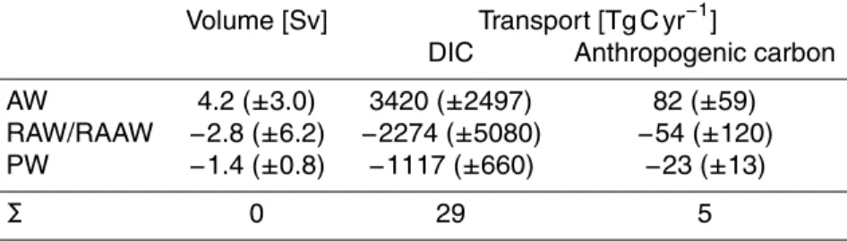
Table 2 shows the transport estimates of DIC and anthropogenic carbon separated 25

(19)

OSD

12, 2189–2229, 2015

T. Stöven et al.

Title Page

Tables Figures

◭ ◮

Back Close

Full Screen / Esc

Discussion

P

a

per

|

Discussion

P

a

per

|

Discussion

P

a

per

|

Discussion

P

a

per

|

Water and the Polar Water of the East Greenland Current. The mean flux of deep water layers below 750 m was taken to be 0 Sv and therefore not considered for this estimate. The water masses were defined as described in Sect. 2.2.

The northwards flux transports 3420±2497 Tg C yr−1 (mean ±standard deviation)

of DIC and 82±59 Tg C yr−1of anthropogenic carbon into the Arctic Ocean. This input

5

is counterbalanced by an export of 2274±5080 Tg C yr−1/54±120 Tg C yr−1by

Recir-culating and Return Atlantic Water and 1117±660 Tg C yr−1/23±13 Tg C yr−1by Polar

Water. The carbon transport uncertainties are relatively high, especially with respect to the error range of the Recirculating/Return water masses of the Atlantic Water. Further-more, there is a lack of water transport data on the Greenland shelf region, e.g. Belgica 10

Bank, and thus we cannot with great confidence decide whether more anthropogenic carbon is transported into or out of the Arctic region through the Fram Strait.

3.8 Uncertainties

The applicability of IG-TTD model at high latitudes, like in the Fram Strait or the South-ern Ocean, is supposed to be limited by complex water mass mixing and ventilation 15

patterns. They should rather be described by more refined models like the maximum entropy method by Holzer and Primeau (2012). The main uncertainty factor is related

to the assumption that diff_{erent saturation states of the transient tracers are}

respon-sible for the tracer age relationships rather than specific mixing processes and that thereby the IG-TTD model is valid for all water masses in the Fram Strait. The uncer-20

tainties of the IG-TTD model depend on the shape of the IG-TTD, i.e. the∆_/Γ _ratio,

and the uncertainties of the boundary conditions and the measurement precision of the transient tracers and apparent transient tracers (see Sect. 3.6 above). The flux es-timates are based on transient tracer and DIC data of the ARK-XXVII/1 cruise which only show the specific distribution pattern during June/July 2012 and thus neglect any 25

(20)

au-OSD

12, 2189–2229, 2015

T. Stöven et al.

Title Page

Tables Figures

◭ ◮

Back Close

Full Screen / Esc

Discussion

P

a

per

|

Discussion

P

a

per

|

Discussion

P

a

per

|

Discussion

P

a

per

|

thors recommend the use of data from the subsurface layer (Vazquez-Rodriguez et al., 2012) or the surface temperature and salinity dependencies (Lee et al., 2006).

The transport estimates are complicated by the fact that the flow field in Fram Strait is dominated by many small scale features. The Rossby radius is 4–6 km which means that the mooring spacing is only able to fully resolve the mesoscale near the shelfbreak 5

in the West Spitsbergen Current. Otherwise, eddies may be aliased between the moor-ings. The velocities in the recirculation area in the center of Fram Strait are actually mostly westward (Beszczynska-Möller et al., 2012) and thus along the mooring array line. Therefore, the meridional velocities in the center of Fram Strait are only the small residuals of much larger zonal velocities. As a result the finite accuracy and precision 10

of the current direction measurements has a big impact on the meridional exchanges. Additionally, at depth the flow is topographically steered, but the topographic features are also not fully resolved. Interannual variations are also neglected here, but they are small (Beszczynska-Möller et al., 2012). The exchange flow across Fram Strait below 750 m (sill depth of Greenland–Scotland ridge and depth horizon of the third instru-15

ments on the moorings) is assumed to be 0 Sv for the present purpose.

4 Conclusions

Measurements of the transient tracers CFC-12 and SF6 along 78

◦

50′N in the Fram

Strait in 2012 show specific characteristics of the diff_{erent water masses. The tracer}

age relationship between both tracers can be separated into two major branches. One 20

branch describes the tracer age relationship of water masses of Atlantic origin as well as deep water masses, the other describes water masses of Arctic origin. We assumed

that the diff_{erent tracer age relationships are due to di}ff_{erent saturation e}ff_{ects on the}

tracers during water mass formation and still existing off_{sets of the SF}₆_{concentrations}

caused by the deliberate tracer release experiment in the Greenland Sea in 1996. The 25

CFC-12 data was saturation corrected by applying the model output of Shao et al.

(21)

OSD

12, 2189–2229, 2015

T. Stöven et al.

Title Page

Tables Figures

◭ ◮

Back Close

Full Screen / Esc

Discussion

P

a

per

|

Discussion

P

a

per

|

Discussion

P

a

per

|

Discussion

P

a

per

|

the IG-TTD which then provides the excess concentrations of SF₆. The largest

ex-cess concentrations of 0.5–0.8 fmol kg−1were found for the intermediate layer between

500 m and 1600 m.

The anthropogenic carbon content was estimated using the IG-TTD and

saturation-corrected CFC-12 data in the ocean interior (depths below 100 m) and SF6in the

sur-5

face layer. The Atlantic Water and Recirculating Atlantic Water is characterized by

an-thropogenic carbon concentrations of 50–55 µmol kg−1 and the Polar Surface Water

by concentrations of 40–45 µmol kg−1. Maximum concentrations of 35–40 µmol kg−1 in

the intermediate layer can be found at 1–3◦W. Deep water layers show decreasing

concentrations with increasing depth from 35 µmol kg−1down to≈10 µmol kg−1.

10

The mean current velocity data obtained by a mooring-array at 78◦50′N between

2002 and 2010 suggests a mean northwards flux of 4.2 (±3.0) Sv of Atlantic Water

(West Spitsbergen Current) and a mean southward flux of 2.8 (±6.2) Sv of

Recirculat-ing/Return Atlantic Water and 1.4 (±0.8) Sv of Polar Water (East Greenland Current).

The net flux of water masses below 750 m was taken to be 0 Sv. The high uncertainties 15

of the flux data in the Fram Strait inhibit any statements about dominating shares of DIC and anthropogenic exports or imports to the Arctic Ocean. However, the flux estimates

indicate a balanced transport budget with a northward flux of 3420 (±2497) Tg C yr−1of

DIC and 82 (±59) Tg C yr−1of anthropogenic carbon by Atlantic Water and a southward

flux of 2274 (±5080) Tg C yr−1/54 (±120) Tg C yr−1by Recirculating and Return Atlantic

20

Water and 1117 (±660) Tg C yr−1/23 (±13) Tg C yr−1by Polar Water.

Acknowledgements. This work was supported by the Deutsche Forschungsgemeinschaft (DFG) in the framework of the priority programme “Antarctic Research with comparative investigations in Arctic ice areas” by a grant to T. Tanhua and M. Hoppema: Carbon and transient tracers dynamics: A bi-polar view on Southern Ocean eddies and the changing Arctic 25

(22)

OSD

12, 2189–2229, 2015

T. Stöven et al.

Title Page

Tables Figures

◭ ◮

Back Close

Full Screen / Esc

Discussion

P

a

per

|

Discussion

P

a

per

|

Discussion

P

a

per

|

Discussion

P

a

per

|

Polarstern, the chief scientist and the scientific party. Special thanks goes to Boie Bogner for his technical support during the ARK-XXVII/1 cruise.

The article processing charges for this open-access publication were covered by a Research Centre of the Helmholtz Association.

5

References

Beszczynska-Möller, A.: The expedition of the research vessel Polarstern to the Arc-tic in 2012 (ARK-XXVII/1), Reports on Polar and Marine Research, 660, 1–78, doi:10.2312/BzPM_0660_2013, 2013. 2192

Beszcynska-Möller, A. and Wisotzki, A.: Physical Oceanography During POLARSTERN Cruise 10

ARK-XXVII/1, Alfred-Wegener-Institute, Helmholtz Center for Polar and Marine Research, Bremerhaven, doi:10.1594/PANGAEA.801791, 2012. 2193, 2197

Beszczynska-Möller, A., Fahrbach, E., Schauer, U., and Hansen, E.: Variability in Atlantic water temperature and transport at the entrance to the Arctic Ocean, 1997-2010, ICES J. Mar. Sci., 69, 852–863, 2012. 2191, 2194, 2208

15

Bullister, J.: Atmospheric Histories (1765–2015) for CFC-11, CFC-12, CFC-113, CCl₄, SF₆ and N₂O, Carbon Dioxide Information Analysis Center, Oak Ridge National Laboratory, US Department of Energy, Oak Ridge, Tennessee, USA, doi:10.3334/CDIAC/otg.CFC_ATM_Hist_2015, 2015. 2196

Bullister, J. L. and Wisegarver, D.: The shipboard analysis of trace levels of sulfur hexafluo-20

ride, chlorofluorocarbon-11 and chlorofluorocarbon-12 in seawater, Deep-Sea Res. Pt. I, 55, 1063–1074, 2008. 2193

de Steur, L., Hansen, E., Mauritzen, C., Beszczynska-Möller, A., and Fahrbach, E.: Impact of recirculation on the East Greenland Current in Fram Strait: Results from moored current meter measurements between 1997 and 2009, Deep-Sea Res., 92, 26–40, 2014. 2191, 25

2194

(23)

OSD

12, 2189–2229, 2015

T. Stöven et al.

Title Page

Tables Figures

◭ ◮

Back Close

Full Screen / Esc

Discussion

P

a

per

|

Discussion

P

a

per

|

Discussion

P

a

per

|

Discussion

P

a

per

|

Eakins, B. and Sharman, G.: Volumes of the World’s Ocean from ETOPO1, NOAA National Geophysical Data Center, Boulder, CO, USA, available at: http://ngdc.noaa.gov/mgg/global/ etopo1_ocean_volumes.html (last access: 22 September 2015), 2010. 2203

Fahrbach, E., Meincke, J., Østerhus, S., Rohardt, G., Schauer, U., Tverberg, V., and Verduin, J.: Direct measurements of volume transports through Fram Strait, Polar Res., 20, 217–224, 5

doi:10.1111/j.1751-8369.2001.tb00059.x, 2001. 2191

Hall, T. M. and Plumb, R. A.: Age as a diagnostic of stratospheric transport, J. Geophys. Res., 99, 1059–1070, 1994. 2195

Holzer, M. and Primeau, F. W.: Improved constraints on transit time distributions from argon 39: A maximum entropy approach, J. Geophys. Res.-Oceans, 115, C12021, 10

doi:10.1029/2010JC006410, 2012. 2207

Huhn, O., Rhein, M., Hoppema, M., and van Heuven, S.: Decline of deep and bottom water ventilation and slowing down of anthropogenic carbon storage in the Weddell Sea, 1984– 2011, Deep-Sea Res. Pt. I, 76, 66–84, doi:10.1016/j.dsr.2013.01.005, 2013. 2195

Johnson, K., Wills, K., Butler, D., Johnson, W., and Wong, C.: Coulometric total carbon dioxide 15

analysis for marine studies: maximizing the performance of an automated gas extraction sys-tem and coulometric detector, Mar. Chem., 44, 167–187, doi:10.1016/0304-4203(93)90201-X, 1993. 2193

Johnson, K. M., Dickson, A. G., Eischeid, G., Goyet, C., Guenther, P., Key, R. M., Millero, F. J., Purkerson, D., Sabine, C. L., Schottle, R. G., Wallace, D. W., Wilke, R. J., and Winn, C. D.: 20

Coulometric total carbon dioxide analysis for marine studies: assessment of the quality of total inorganic carbon measurements made during the US Indian Ocean CO₂Survey 1994-1996, Mar. Chem., 63, 21–37, doi:10.1016/S0304-4203(98)00048-6, 1998. 2193

Jutterström, S. and Jeansson, E.: Anthropogenic carbon in the East Greenland Current, Prog. Oceanogr., 78, 29–36, doi:10.1016/j.pocean.2008.04.001, 2008. 2205

25

Karcher, M., Smith, J. N., Kauker, F., Gerdes, R., and Smethie, W. M.: Recent changes in Arctic Ocean circulation revealed by iodine-129 observations and modeling, J. Geophys. Res.-Oceans, 117, C08007, doi:10.1029/2011JC007513, 2012. 2194

Kurtz, N., Markus, T., Farrell, S., Worthen, D., and Boisvert, L.: Observations of recent Arctic sea ice volume loss and its impact on ocean-atmosphere energy exchange and ice production, 30

(24)

OSD

12, 2189–2229, 2015

T. Stöven et al.

Title Page

Tables Figures

◭ ◮

Back Close

Full Screen / Esc

Discussion

P

a

per

|

Discussion

P

a

per

|

Discussion

P

a

per

|

Discussion

P

a

per

|

Kwok, R., Cunningham, G., Wensnahan, M., Rigor, I., Zwally, H., and Yi, D.: Thinning and volume loss of the Arctic Ocean sea ice cover: 2003-2008, J. Geophys. Res.-Oceans, 114, C07005, doi:10.1029/2009JC005312, 2009. 2191

Law, C. S., Watson, A. J., and Liddicoat, M. I.: Automated vacuum analysis of sulphur hexafluo-ride in seawater: derivation of the atmospheric trend (1970-1993) and potential as a transient 5

tracer, Mar. Chem., 48, 57–69, 1994. 2193

Lee, K., Tong, L., Millero, F., Sabine, C., Dickson, A., Goyet, C., Park, G., Wanninkhof, R., Feely, R., and Key, R.: Global relationships of total alkalinity with salinity and tem-perature in surface waters of the worlds oceans, Geophys. Res. Lett., 33, L19605, doi:10.1029/2006GL027207, 2006. 2208

10

Liang, J.-H., Deutsch, C., McWilliams, J. C., Baschek, B., Sullivan, P. P., and Chiba, D.: Param-eterizing bubble-mediated air-sea gas exchange and its eff_{ect on ocean ventilation, Global} Biogeochem. Cy., 27, 894–905, doi:10.1002/gbc.20080, 2013. 2203

MacGilchrist, G., Naveira Garabato, A., Tsubouchi, T., Bacon, S., Torres-Valdes, S., and Azetsu-Scott, K.: The Arctic Ocean carbon sink, Deep-Sea Res. Pt. I, 86, 39–55, 15

doi:10.1016/j.dsr.2014.01.002, 2014. 2192, 2196

Marnela, M., Rudels, B., Houssais, M.-N., Beszczynska-Möller, A., and Eriksson, P. B.: Recir-culation in the Fram Strait and transports of water in and north of the Fram Strait derived from CTD data, Ocean Sci., 9, 499–519, doi:10.5194/os-9-499-2013, 2013. 2191

Mintrop, L., Pérez, F. F., González-Dávila, M., Santana-Casiano, J. M., Körtzinger, A.: Alkalinity 20

determination by potentiometry: intercalibration using three diff_{erent methods, Cienc. Mar.,} 26, 23–37, 2000. 2193

Olsson, K. A., Jeansson, E., Tanhua, T., and Gascard, J.-C.: The East Greenland Cur-rent studied with CFCs and released sulphur hexafluoride, J. Marine Syst., 55, 77–95, doi:10.1016/j.jmarsys.2004.07.019, 2005. 2203

25

Polyakov, I., Beszczynska, A., Carmack, E., Dmitrenko, I., Fahrbach, E., Frolov, I., Gerdes, R., Hansen, E., Holfort, J., Ivanov, V., Johnson, M., Karcher, M., Kauker, F., Morison, J., Orvik, K. A., Schauer, U., Simmons, H., Skagseth, Ø., Sokolov, V., Steele, M., Timokhov, L., Walsh, D., and Walsh, J.: One more step toward a warmer Arctic, Geophys. Res. Lett., 32, L17605, doi:10.1029/2005GL023740, 2005. 2191

30

(25)

OSD

12, 2189–2229, 2015

T. Stöven et al.

Title Page

Tables Figures

◭ ◮

Back Close

Full Screen / Esc

Discussion

P

a

per

|

Discussion

P

a

per

|

Discussion

P

a

per

|

Discussion

P

a

per

|

Yermak Plateau in summer 1997, Ann. Geophys., 18, 687–705, doi:10.1007/s00585-000-0687-5, 2000. 2197

Rudels, B., Björk, G., Nilsson, J., Winsor, P., Lake, I., and Nohr, C.: The interaction between waters from the Arctic Ocean and the Nordic Seas north of Fram Strait and along the East Greenland Current: results from the Arctic Ocean-02 Oden expedition, J. Marine Syst., 55, 5

1–30, doi:10.1016/j.jmarsys.2004.06.008, 2005. 2197

Rudels, B., Marnela, M., and Eriksson, P.: Constraints on estimating mass, heat and freshwater transports in the Arctic Ocean: an exercise, in: Arctic-Subarctic Ocean Fluxes, edited by: Dickson, R., Meincke, J., and Rhines, P., Springer Netherlands, 315–341, doi:10.1007/978-1-4020-6774-7_14, 2008. 2191

10

Rudels, B., Korhonen, M., Budéus, G., Beszczynska-Möller, A., Schauer, U., Nummelin, A., Quadfasel, D., and Valdimarsson, H.: The East Greenland Current and its impacts on the Nordic Seas: observed trends in the past decade, ICES J. Mar. Sci., 69, 841–851, doi:10.1093/icesjms/fss079, 2012. 2191

Schauer, U. and Beszczynska-Möller, A.: Problems with estimation and interpretation of 15

oceanic heat transport – conceptual remarks for the case of Fram Strait in the Arctic Ocean, Ocean Sci., 5, 487–494, doi:10.5194/os-5-487-2009, 2009. 2191

Schauer, U., Fahrbach, E., Østerhus, S., and Rohardt, G.: Arctic warming through the Fram Strait: oceanic heat transport from 3 years of measurements, J. Geophys. Res.-Oceans, 109, C06026, doi:10.1029/2003JC001823, 2004. 2191

20

Schauer, U., Beszczynska-Möller, A., Walczowski, W., Fahrbach, E., Piechura, J., and Hansen, E.: Variation of measured heat flow through the Fram Strait between 1997 and 2006, in: Arctic-Subarctic Ocean Fluxes, edited by: Dickson, R., Meincke, J., and Rhines, P., Springer Netherlands, 65–85, doi:10.1007/978-1-4020-6774-7_4, 2008. 2191

Schneider, A., Tanhua, T., Koertzinger, A., and Wallace, D.: High anthropogenic carbon content 25

in the eastern Mediterranean, J. Geophys. Res., 115, C12050, doi:10.1029/2010JC006171, 2010. 2195

Schneider, A., Tanhua, T., Roether, W., and Steinfeldt, R.: Changes in ventilation of the Mediter-ranean Sea during the past 25 year, Ocean Sci., 10, 1–16, doi:10.5194/os-10-1-2014, 2014. 2195

30

(26)

OSD

12, 2189–2229, 2015

T. Stöven et al.

Title Page

Tables Figures

◭ ◮

Back Close

Full Screen / Esc

Discussion

P

a

per

|

Discussion

P

a

per

|

Discussion

P

a

per

|

Discussion

P

a

per

|

Sonnerup, R., Mecking, S., and Bullister, J.: Transit time distributions and oxygen utilization rates in the Northeast Pacific Ocean from chlorofluorocarbons and sulfur hexafluoride, Deep-Sea Res. Pt. I, 72, 61–71, doi:10.1016/j.dsr.2012.10.013, 2013. 2200

Stöven, T. and Tanhua, T.: Ventilation of the Mediterranean Sea constrained by multiple tran-sient tracer measurements, Ocean Sci., 10, 439–457, doi:10.5194/os-10-439-2014, 2014. 5

2193, 2200

Stöven, T., Tanhua, T., Hoppema, M., and Bullister, J. L.: Perspectives of transient tracer ap-plications and limiting cases, Ocean Sci., 11, 699–718, doi:10.5194/os-11-699-2015, 2015. 2200, 2203, 2206

Stroeve, J., Serreze, M., Drobot, S., Gearheard, S., Holland, M., Maslanik, J., Meier, W., and 10

Scambos, T.: Arctic sea ice extent plummets in 2007, EOS T. Am. Geophys. Un., 89, 13–14, doi:10.1029/2008EO020001, 2008. 2191

Tanhua, T., Bulsiewicz, K., and Rhein, M.: Spreading of Overflow Water from the Greenland to the Labrador Sea, Geophys. Res. Lett., 32, L10605, doi:10.1029/2005GL022700, 2005. 2203

15

Tanhua, T., Waugh, D. W., and Wallace, D. W. R.: Use of SF₆to estimate anthropogenic CO₂ in the upper ocean, J. Geophys. Res., 113, 2156–2202, doi:10.1029/2007JC004416, 2008. 2191, 2195, 2202, 2204

Tans, P. and Keeling, R.: Full Mauna Loa CO₂ record, NOAA/ESRL, available at: www.esrl. noaa.gov/gmd/ccgg/trends/, last access: 22 September, 2015. 2196

20

Tsubouchi, T., Bacon, S., Naveira Garabato, A. C., Aksenov, Y., Laxon, S. W., Fahrbach, E., Beszczynska-Möller, A., Hansen, E., Lee, C. M., and Ingvaldsen, R. B.: The Arctic Ocean in summer: a quasi-synoptic inverse estimate of boundary fluxes and water mass transforma-tion, J. Geophys. Res.-Oceans, 117, C01024, doi:10.1029/2011JC007174, 2012. 2192 van Heuven, S., Pierrot, D., Rae, J., Lewis, E., and Wallace, D.: MATLAB Program De-25

veloped for CO₂ System Calculations, Carbon Dioxide Information Analysis Center, Oak Ridge National Laboratory, US Department of Energy, Oak Ridge, Tennessee, USA, doi:10.3334/CDIAC/otg.CO2SYS_MATLAB_v1.1, 2011. 2196

Vazquez-Rodriguez, M., Padin, X., Pardo, P., Rios, A., and Perez, F.: The subsurface layer reference to calculate preformed alkalinity and air-sea CO₂ disequilibrium in the Atlantic 30

Ocean, J. Marine Syst., 94, 52–63, 2012. 2208