Maximize the Effects of Growth Factors in PC12 Cells
Kazunari Mouri¤, Yasushi Sako*
Cellular Informatics Laboratory, RIKEN, 2-1 Hirosawa, Wako 351-0198, Saitama, Japan
Abstract
Recently, the heterogeneity that arises from stochastic fate decisions has been reported for several types of cancer-derived cell lines and several types of clonal cells grown under constant environmental conditions. However, the relation between this stochasticity and the responsiveness to extracellular stimuli remains largely unknown. Here we focused on the fate decisions of the PC12 cell line, which was derived from rat pheochromocytoma, and is a model system to study differentiation into sympathetic neurons. Whereas epidermal growth factor (EGF) stimulates the proliferation of populations of PC12 cells, nerve growth factor (NGF) promotes the differentiation of neurites to neuron-like cells. We found that phenotypic heterogeneity increased with time at several surrounding serum concentrations, suggesting stochastic cell-fate decisions in single cells. We made a simple mathematical model assuming Markovian transitions of the cell fates, and estimated the transition rates based on Bayes’ theorem. The model suggests that depending on the serum concentration, EGF (NGF) even directs differentiation (proliferation) at the single-cell level. The maximum effects of the growth factors were ensured when the transition rates were appropriately controlled by the serum concentration to produce a nonextremal, moderate amount of cell-fate heterogeneity. Our model was validated by the experimental finding that the means and variances of the local cell densities obey a power-law relationship. These results suggest that even when efficient responses to growth factors are observed at the population level, the growth factors stochastically direct the cell-fate decisions in different directions at the single-cell level.
Citation:Mouri K, Sako Y (2013) Optimality Conditions for Cell-Fate Heterogeneity That Maximize the Effects of Growth Factors in PC12 Cells. PLoS Comput Biol 9(11): e1003320. doi:10.1371/journal.pcbi.1003320
Editor:Stanislav Shvartsman, Princeton University, United States of America
ReceivedMarch 7, 2013;AcceptedSeptember 16, 2013;PublishedNovember 14, 2013
Copyright:ß2013 Mouri, Sako. This is an open-access article distributed under the terms of the Creative Commons Attribution License, which permits unrestricted use, distribution, and reproduction in any medium, provided the original author and source are credited.
Funding:This work was supported by a RIKEN’s Basic Science Interdisciplinary Research Project ‘‘Cellular Systems Biology’’. The funders had no role in study design, data collection and analysis, decision to publish, or preparation of the manuscript.
Competing Interests:The authors have declared that no competing interests exist. * E-mail: [email protected]
¤ Current address: Laboratory for Cell Polarity Regulation, RIKEN Quantitative Biology Center, Suita, Japan.
Introduction
Phenotypic heterogeneity, which has been thoroughly discussed for tumor cells, is not a unique property of cancerous cells but has also been observed in normal clonal cells in culture [1]. Differences in tumor cells have been attributed to differences in cell lineages that arise from genetic or epigenetic processes. However, even clonal cells show phenotypes that are certainly not identical because they are subject to various sources of stochasticity other than genetic heterogeneity [2]. Recent insights have suggested that molecular ‘noise’ caused by fluctuations in gene expression, signal transduction, and other processes affects phenotypic heterogeneity in organisms ranging from microbes to mammals [3]. In the presence of such noise, even cells with the same overall phenotypic profile fluctuate randomly, causing them to have subtly different phenotypes at any particular time. This is a key mechanism that generates the cellular diversity that is sometimes used as bet-hedging of bacterial persistence in Escherichia colior competence inBacillus subtilis[4,5]. In mammals, several types of cells use stochastic decision-making to regulate development [6–10].
Although heterogeneity was observed in several types of cells, the effects of extracellular stimuli on those heterogeneous populations have not been fully clarified. Here, we used PC12
cells to attempt to address this issue. The rat pheochromocytoma clone PC12, which was developed from an adrenal medullary tumor derived from the adrenergic neural crest [11], has been used as a model of neural differentiation. Healthy PC12 cells can be grown under appropriate content percentage of serum in a medium for culture, and they have several properties that resemble those of adrenal medullary chromaffin cells [12]. In the presence of nerve growth factor (NGF), PC12 cells stop dividing, display electrical excitability, produce neurite-like out-growths, and differentiate into cells with a sympathetic neuron-like phenotype. Although the removal of NGF for sympathetic neurons leads to cell death, the differentiation of PC12 cells appears to be reversible insofar as removal of NGF causes them to lose the properties acquired after differentiation. It has been reported that the effects of NGF on differentiation are efficient under serum-starved conditions [13]. The epidermal growth factor (EGF) receptor is also expressed in PC12 cells [12]. As in other cell types [14], EGF acts as a mitogen in PC12 cells [15]. However, the effect of EGF can be masked by culture conditions, especially the content percentage of serum [15].
measured quantitatively. Here, we report the effects of the growth factors EGF and NGF under three different serum conditions, in which PC12 cells show different degrees of heterogeneity in their fate decisions. We measured the time courses of the numbers of cells in three states (proliferating, differentiated, and dead) and constructed a mathematical model. By definition, we regard concentrations of surrounding serum as an environmental condition, and regard cell responses as meaning changes in cell fate triggered by stimuli, such as EGF and NGF, at that particular serum concentration.
In this study, we first used entropy values to define the heterogeneity of a population of cells containing a large fraction of proliferative cells, and found that the entropy values increased as a function of time, suggesting that stochastic cell-fate decisions in single PC12 cells increased the heterogeneity of the population, regardless of the surrounding serum. This heterogeneity decreased as the concentration of the surrounding serum increased. We made a simple mathematical model assuming that cells determine their fates with constant probabilities, and estimated the proba-bilities for which the model can explain the experimental results, based on Bayes’ theorem. This method enabled us to use experimental data collected using populations of cells to estimate the rates with which single cells made cell-fate decisions. Based on the model and the parameter values, we redefined the effects of the growth factors: EGF increased the proliferation rate at the single-cell level, although the effect could be covered and was affected by the surrounding serum at the population level, as shown in previous experiments. At some serum concentrations, EGF (NGF) even directed differentiation (proliferation) at the single-cell level. Even when efficient responses to the growth factors were observed at the population level, the growth factors only stochastically directed single cells to different cell fates. We evaluated the strength of the responses to the growth factors at the population level on a phase portrait using the Malthus coefficient and the fluxes of the three phenotypes, and examined the relationship between cell heterogeneity and cell responsiveness. The strength of the responses to EGF and NGF as a function of entropy (cell-fate heterogeneity) peaked at a moderate entropy value. Finally, we
showed that the relationship between the means and variances of the local cell densities obeyed a power-law relationship, which could be explained by a stochastic simulation that supported the idea that the cells have a single set of transition rates with constant values under each condition.
Results/Discussion
Cell-fate decisions rate in single PC12 cells
In this section, we first report experimental results that describe dynamic changes in the number of cells at the population level. Next, we propose the use of a mathematical model to calculate transition rates at the single cell level from experimental results.
Heterogeneity of cellular states in cell
populations. Three typical states of PC12 cells are defined by their morphologies (Figure 1 and Materials and methods); These are (1) proliferating cells, which have a rounded shape and can potentially reproduce, differentiate, or die; (2) differentiated cells, which have neurite-like protrusions and can potentially de-differentiate or die; and (3) dead cells, which are recognized by the presence of cellular debris. The proliferating PC12 cells were passaged into culture dishes at initial densities of 20{50cells=mm2. The cells did not reach confluence (over 500cells=mm2) in the five days of our experimental period. We
measured the mean densities of each of the three phenotypically distinct populations in culture daily in30randomly selected fields in a single dish (Figure 1).
We compared the cell-fate processes under control conditions, in which the cells were cultured without additional growth factors but in the presence of three different concentrations of serum (Figures 2A, D, and G). In the presence of high serum concentrations (10%horse serum (HS) and5%fatal bovine serum (FBS); which is the normal serum concentration used to culture PC12 cells) proliferated efficiently (approximately 90% of cells were proliferating) and grew exponentially. However, even in the presence of a high serum concentration, the number of cells that differentiated or died also increased, maintaining constant fractions (*10%). In the presence of a low serum concentration (0:1% HS, 0:05% FBS), the number of proliferating cells was almost constant, and the number and fraction of differentiated or dead cells increased. Under the serum-free condition (culture medium containing1%bovine serum albumin (BSA)), the number of proliferating cells decreased, whereas the numbers of dead and differentiated cells increased. Specifically, the fraction of differen-tiated cells increased4:9-fold or 7:7-fold following growth under low-serum conditions or serum-free conditions, respectively, compared with the fraction under high-serum conditions. There-fore, even under the control conditions, a population of cells became heterogeneous with time under low-serum and serum-free conditions. To explicitly evaluate the extent to which cell fates within a population become heterogeneous, we introduced Shannon entropy (S), and calculated the time-dependent entropy
S(t)in Figure 3A.
S~{P(x)lnP(x){P(y)lnP(y){P(z)lnP(z),
whereP(x),P(y), andP(z) are the fractions of cells of each cell fate, andP(x)zP(y)zP(z)~1. The maximum value of entropy isSmax&1:10 for P(x)~P(y)~P(z)~0:33, the middle value is
Shalf&0:69forP(x)~P(y)~0:50andP(z)~0, for example, and the minimum value isSmin~0for P(x)~1and P(y)~P(z)~0, for example. When the value of entropy is SvShalf, the heterogeneity of a population is small and the cell population largely follows a single fate. In contrast, if the fate decision of Author Summary
individual cells is random, the cells become heterogeneous and the value of entropy increases to Smax. In Figure 3A, we show the entropy values as a function of time for the three control-serum conditions. At the high serum concentration, entropy was sustained at a low value of approximately 0:4 because a large fraction of cells were proliferating. Under serum-free conditions, a rapid increase in entropy was observed, and the entropy approached the maximum value (Smax), exceeding its middle value (Shalf), indicating the high heterogeneity of the cell population. In the presence of a low serum concentration, a
moderate increase in entropy was observed, and the value was close to Shalf. Therefore, cell heterogeneity depended on the concentration of the surrounding serum and increased as the serum concentration decreased. Cell-fate decisions displayed the greatest uncertainty under serum-free conditions, in which cells not only died but also differentiated to generate a heterogeneous population. Even at high serum concentrations, a small number of cells differentiated or died.
The growth factor EGF was added to these control conditions to evaluate how cell-fate decisions change in response to this stimulus (Figure 2B, E, and H). A saturated concentration of EGF (100ng=ml) was used. Although EGF is known to induce cell proliferation, the number of proliferating cells did not explicitly increase in the high-serum concentration in the presence of EGF when compared with the control condition. In the presence of low-serum concentrations, slight increases in the number of prolifer-ating cells were detected in the presence of EGF, but differenti-ation was also clearly accelerated. Under serum-free conditions, proliferating cells decreased even in the presence of EGF. Therefore, the responses of cells to the EGF stimulus depended on the concentration of surrounding serum. This suggests that EGF not only affects the proliferation of cells, but also affects their differentiation, although the effects of EGF on cell death were obscure for all of the serum conditions tested.
When we added the growth factor NGF, differentiation was accelerated under all of the serum conditions tested (Figure 2C, F, and I). A saturated concentration of NGF (50ng=ml) was used. Under high-serum conditions, the number of proliferating cells was sustained for a week in the presence of NGF, whereas it increased under control conditions. Thus, both the number and proportion of differentiated cells increased. NGF did not completely suppress cell death, as shown by the increased number of dead cells. However, under the low-serum condition, the number of proliferating cells decreased as the number of differentiated cells increased. In contrast, the number of prolifer-ating cells remained constant with a slight increase of the number of differentiated cells under control conditions. The sustained composition of the surviving cells resulted from NGF-mediated stimulation of the transition of the proliferating cells into differentiated cells. Under serum-free conditions, changes in the numbers of proliferating cells over time were similar in the presence or absence of NGF, but the number of differentiated cells was larger in the presence of NGF than in its absence. This result indicates that the number of surviving cells gradually decreases upon exposure to NGF, which increases the proportion of differentiated cells.
Therefore, in our experiments, cell death and differentiation were not completely suppressed under conditions that support logarithmic growth, and cells differentiate without any growth factors even under serum-free conditions. Thus, the clonal PC12 cells became a heterogeneous population under each of the serum conditions tested. In addition, the effects of EGF and NGF depended on the environmental serum conditions, with both of these growth factors affecting multiple transition pathways. To further validate this issue, we generated a mathematical model to capture these stochastic state transitions of PC12 cells. This model is discussed in the section that follows.
Single-cell-level state transition rates derived from a mathematical model. It is difficult to evaluate and compare the processes that determine the fates of single cells quantitatively among different conditions directly from monitoring changes in the number of cells over time. For quantification, we constructed a mathematical model that uses ordinary differential equations to capture the state transitions of cells (Figure 1A and Models
Figure 1. Fates of PC12 cells and experimental procedures.(A)
The three typical states of PC12 cells. Whereas proliferating cells are usually rounded, differentiated cells have extended neurites, and dead cells are recognized as shrunken or fragmented cell bodies. EGF, epidermal growth factor; NGF, nerve growth factor. The values of proliferating (x), differentiated (y), and dead (z) cells denote densities of each cell. Five parameters describe the transition rates of proliferation (m), differentiation (k1), de-differentiation (k2), cell death fromx(d1), and
cell death fromy(d2). We made a mathematical model of differential
equations and estimated those five parameters using Bayesian inference. Details are shown in the Models section. (B) The experimental procedures used involved photographing randomly sampled places (0:14or0:57mm2) on a dish, and then counting the numbers of cells
with features of each of the three states defined above. Means (m~PMi~1ni=M) and variances (s2~PMi~1(ni{m)2=(M{1)) of the number of cells in each state were calculated by analysis of the entire surface of each dish.
section). We assumed that the observed heterogeneity of a population is caused by the stochastic fate decisions of single cells. In this model, transition rates describe the probabilities that the phenotypes of cells may change. We estimated the values of the transition rates in the experimental data based on Bayes’ theorem and evaluated the effects of serum and growth factors. Estimated results based on the experiments in Figure 2 are shown in Table S1, and time courses of this model using these parameters successfully fitted most of the experimental results (Figure 2). Therefore, our state transition model can explain our experimen-tal results by modifying parameter values of the model, suggesting that the structure of the model is valid where we did not consider cell–cell interactions.
We carried out four independent sets of experiments and predicted parameter values for each experiment. The mean parameter values enabled us to estimate typical characteristics of cell-fate decisions in single PC12 cells. State transition rates at the single-cell level were compared among control conditions (Figure 4 and Figure S1). In the high-serum concentration, we can easily estimate the doubling time td&40h from the proliferation rate
m&0:4day{1. Even if cells differentiate, they immediately
de-differentiate or die, with slow inductions of differentiation and death, resulting in a low entropy value (Figure 3). At the low serum concentration, the proliferation occurs with slow induction of differentiation and comparatively fast induction of death, which
results in an intermediate entropy level (Figure 3). Under serum-free conditions, cells slowly proliferate with inducing differentia-tion and death, which results in a high entropy value (Figure 3). Each parameter had a nonzero value, regardless of the environ-mental serum conditions, and the values for entropy gradually increased under low-serum and serum-free conditions.
In Figure 4A–E, we show the parameter values for three environmental serum conditions in the presence or absence of either EGF or NGF. Both growth factors affected several transition pathways. For example, they drove both proliferation and differentiation, whereas for other transitions their effects depended on the environmental serum conditions. Whereas EGF increased the proliferation ratemfor all serum conditions, NGF increased the differentiation ratek1for all serum conditions. However, we found that NGF increased the proliferation ratemin the presence of serum, and the differentiation ratek1was increased affected by EGF for all serum conditions at the single-cell level. It has been suggested that although EGF is a mitogen for PC12 cells, and is capable of moderate stimulation of the proliferation of PC12 cells, these effects might be masked by serum conditions used for cell culture [15]. At the population level (Figure 2), it was unclear whether EGF affected cellular proliferation of cells. However, a mathematical model enabled us to derive transition rates at the single-cell level and to show that EGF stimulated the proliferation rate for all serum conditions, with the magnitude of the increase in Figure 2. Time courses showing changes in the numbers of cells in the presence or absence of epidermal growth factor (EGF) or
nerve growth factor (NGF).Time courses of three cell states were observed in experiments (circular dots), and fitted simulation results (lines) for
the high serum (A–C), low serum (D–F), and serum free (G–I) conditions in the presence or absence of EGF or NGF. For each experiment, we counted
100{1000cellsto calculate the average number of cells for each day. Typical results of four independent experiments in each condition are shown. The parameters in Table S1 were applied to simulate a mathematical model. For each figure, lines denote the average number of proliferating (red), differentiated (blue), and dead (green) cells. Error bars denote99%confidential region fitted by exponential distribution. HS, horse serum; FBS, fetal bovine serum.
proliferation with respect to the rates of proliferation under control conditions increasing as the concentration of serum decreased, as reported previously [15].
It has usually been suggested that NGF has an antimitogenic effect on PC12 cells [15,16], although NGF has a mitogenic effect on cells purified from late-passage cultures of lines derived from PC12 cells [16]. Analysis of cell numbers failed to reveal any mitogenic activity of NGF (Figure 2), although the proliferation ratemwas higher in the presence of NGF compared with control conditions in high and low serum levels. A model enabled us to calculate the proliferation rate in order to distinguish proliferating cells from differentiated cells that cannot proliferate. This indicates efficient proliferation of PC12 cells in certain conditions with NGF, compared with control conditions, although large rates of differentiation mask the stimulation of proliferation in cell populations.
We also found that EGF stimulated the differentiation ratek1in addition to its mitogenic activity. Previous work [17] revealed that EGF triggered neuronal differentiation of PC12 cells when EGF receptors were overexpressed. In our work, we did not perform genetic manipulations. It seems that stimulation of differentiation is an intrinsic property of PC12 in response to EGF, and that its strength depends on the level of expression of the EGF receptor.
The responses of the de-differentiation ratek2to growth factors are not yet well established. In our research,k2increased in the presence of EGF at the high serum concentration tested. This suggests that the number of proliferating cells increased efficiently even when differentiation occurs. In the presence of NGF, k2
decreased compared to the control condition, and the differenti-ated cells efficiently increased. At the low serum concentration tested, both EGF and NGF decreased the de-differentiation rate
k2, but thek2values for both EGF and NGF (including the control condition) were very small and had minimal effect on decisions related to cell fate. For the serum free condition, the de-differentiation ratek2increased in a presence of NGF, suggesting inefficient differentiation. These results indicate that the effects of EGF and NGF on rates of de-differentiation depend on the serum concentration.
Suppression of cell death by NGF in serum-free medium at the cell-population level was reported previously [18]. Our approach enabled us to estimate single-cell-level responses, and we could calculate the two distinct cell death rates of proliferating and differentiated cells which could not be separated without using a mathematical model. Under high-serum and serum-free
condi-Figure 3. Changes in entropy with time.(A) Serum conditions used
were 10% horse serum (HS) and5%fetal bovine serum (FBS) (black),
0:1%HS and 0:05%FBS (red), and1%BSA (blue). The definition of entropy isS~{P(x)lnP(x){P(y)lnP(y){P(z)lnP(z). The dots show the experimental results and the lines are the results of simulation. The maximum entropy value (Smax&1:10) was determined for when
P(x)~P(y)~P(z)~0:33, and the middle entropy value (Shalf&0:69)
was determined for when P(x)~P(y)~0:50 and P(z)~0. The parameter values in Table S1 were used for the simulations. (B) Under serum-free conditions, the entropy was high, and the numbers of the three cell types on the dish were similar. Under low-serum conditions, levels of entropy were intermediate, and most of the cells were either proliferating or dead. Under high-serum conditions, most of the cells were proliferating.
doi:10.1371/journal.pcbi.1003320.g003
Figure 4. Mean estimated parameters for several serum or
growth factor conditions. (A–E) Individual experiments were
repeated four times (means and standard errors are shown). We applied a simple one-sidedt–test with reference to a serum condition of 10% HS and 5% FBS, and calculated p–values. Asterisks denote
pv0:05. In addition, we marked ‘zz’ or ‘{{’ on the bars for the effect sizedw0:8, and ‘z’ or ‘{’ fordw0:5 (the definition ofd is shown in the Materials and Methods section). The plus (zz, z) or minus ({{,{) marks denote increase or decrease of mean parameter values compared with the control conditions, respectively. Details are shown in the Materials and methods section. (F) Diagrams of the responses to epidermal growth factor (EGF) and nerve growth factor (NGF) for each parameter are shown. The three sequential marks (zzz, and so on) are for the high serum (10%horse serum (HS) and
5%fetal bovine serum (FBS)) the low serum (0:1%HS and0:05%FBS), and the serum free (1%bovine serum albumin) conditions, respectively. The mark ‘z’ (‘{’) indicates increase (decrease) compared with the control conditions, and ‘.’ denotes the absence of statistically significant differences between the parameter values.
tions, the death rate of proliferating cellsd1from the proliferating cells decreased when EGF or NGF were added. Nonetheless, in general, the reagents had minimal effects on the death rate of differentiated cellsd2. In contrast, when the serum concentration was high, NGF increased the death rated1, and both NGF and (to a lesser extent) EGF decreased the death rated2. Therefore, we found that the suppression of cell death depended on serum conditions. Under serum-starved conditions, the growth factors EGF and NGF suppressed the death of proliferating cells, and under high-serum conditions, they suppressed the death of differentiated cells. The suppression of cell death was the combined effect of these two pathways, and these findings could not be achieved in the previous population level experiments that did not use mathematical models [18].
Furthermore, using a mathematical model of differential equations, uu_~Auin equation (4), we can intuitively capture the time courses of the numbers of cellsu(t)~(x(t),y(t))trin a phase portrait (Figure S2). The number of dead cells z(t) does not explicitly affect the number of cellsu(t), but it is implicitly included in the rate constants d1 and d2. According to the simple assumptions of our model, cells under any initial set of conditions (x0,y0) converge to the origin or diverge to infinity along one of the eigenvectors. We calculated phase portraits from individual parameter sets to understand the global features of the population dynamics. To validate the characteristics of the model, we performed an experiment to confirm that the cell-fate dynamics depend on the initial conditions (Figure S3). As predicted by the model, a number of cells moved along the vector fields in the phase plane, and finally converged to one of the eigenvectors. This result supports our assumptions that cell–cell interactions do not dramatically influence the cell-fate dynamics.
Relationships between heterogeneity and responses to growth factors at the population level
The parameter values estimated in the previous section denote single-cell-level transition rates. However, at the population level, the effects of these parameters are very complex (see Models section), and it is difficult to evaluate the effects of the growth factors on the population dynamics from the estimated parameter values. In this section, we introduce a method to use a phase portrait to capture dynamic changes in the number of cells at the population level, and to compare the responses to growth factors under three serum conditions. We use this portrait to quantita-tively characterize the responses to growth factors. Finally, we evaluate the relationships between the heterogeneity of a population and the response indexes.
Population-level validity of a state-transition model. We now introduce some indexes to quantify the direction of cell fate decision processes derived from a mathematical model. In the following section, we evaluate the extent of responses to growth factors compared with the control conditions that use these indexes. We propose three indices. The first is the Malthusian coefficientl, which denotes an asymptotic convergence (lv0) or divergence (lw0) speed of change in the number of cells (details are shown in Models section). In Figure 5A, we show the calculated values of the Malthus coefficients. As indicated by the result of the previous section, a positive effect of a growth factor EGF was evident in the low serum condition. In the presence of NGF, the Malthus coefficients l decreased compared with the control conditions for all serum concentrations. Only when the differentiation ratek1and the proliferation ratemare balanced in addition to lNGFv0 will efficient differentiation occur (Figure S2C, F, and I). Thus, consideration of the asymptotic growth rates
and the results in the previous section suggests that the growth factors EGF and NGF efficiently affect decision processes that affect cell fate at a low serum concentration.
As the second and the third indices, we used the initial fluxJn(0) (n~x,y,z) (see equation (9) in the Models section) and the mean fluxJn~Ð0TJn(t)dt(whereTdenotes an upper limit of calculating the mean flux) of cell fate processes (Figures 5B–G). The unit of those fluxes is cells/mm2/day. These two indices expressed similar results in response to growth factors. For the proliferating cells, EGF had a positive effect on both fluxes of cell fate decision processesJx(0)andJxcompared with the control condition only at the low serum concentration. In the high serum and the serum-free conditions, the apparent effects of EGF were not detected. In contrast, NGF had a negative effect on both fluxes for all serum concentrations. Whereas the effect of EGF depended on the environmental conditions, that of NGF was independent of the
Figure 5. Malthusian coefficient (l) and fluxes (Jn(0)andJn(0))
calculated from phase portraits. Malthusian coefficient (A) and
fluxes (B–G) were calculated using estimated parameters in Table S1. Calculations were made in the presence or absence of growth factors for three environmental serum conditions (10%horse serum (HS) and
5%fetal bovine serum (FBS), 0:1%HS and0:05%FBS, and1%BSA). Fluxes were expressed ascells=mm2=day. The symbols ‘?’, ‘z’, ‘{’,
‘zz’, and ‘{{’ denote the same meanings as those defined in Figure 4. (H) Diagrams of the responses to epidermal growth factor (EGF) and nerve growth factor (NGF) for Malthusian coefficient and fluxes are shown. Three sequential marks (zzz, and so on) denote the same meanings of Figure 4F. The means of four independent experiments are shown with their standard errors.
environmental conditions. For the differentiated cells, the fluxes
Jy(0) and Jy increased in the presence of both growth factors compared with control conditions. Therefore, EGF can become a differentiation factor at a population level, which is consistent with the increase in the parameterk1in the presence of EGF, although the positive effects of NGF on the fluxesJy(0)andJywere larger than those of EGF for all serum conditions (Figure 4B). For the dead cells, the fluxJz(0)decreased under the serum-free and the low-serum conditions in the presence of EGF or NGF, and the mean fluxJz decreased in the presence of NGF.
The effects of growth factors are summarized in Figure 5H. Whereas NGF reduced the flux of proliferating cells, it increased the flux of differentiated cells and suppressed cell death relative to that under control conditions especially under the serum-free and low-serum conditions. Not only did EGF increase the flux of proliferating cells when the serum concentration was low, but it also increased the flux of differentiated cells for all serum conditions. EGF suppressed the initial flux of cell death (Jz(0)) compared with control conditions as it is also suggested in the presence of NGF, but EGF did not affect the mean flux of cell death (Jz). We compare the results between single and a population of PC12 cells (Figure 4F and Figure 5H). As has been suggested in ref [15], the mitogenic activity in response to EGF for a population of cells depended on concentrations of surrounding serum, and it was masked in the high-serum condition. We showed the mitogenic effects of EGF for all the serum concentrations only after we estimated parameter values of proliferating cells in single PC12 cells. In addition, we could reveal antimitogenic effects of NGF in the fluxes of a population of cells, which is consistent with the results in refs [15,19]. We found mitogenic effects of NGF in single PC12 cells, which means that NGF promotes both proliferation and differentiation compared with the control conditions.
Efficient growth factor responses in a moderately heterogeneous cell population. We next compare the strength of responses to growth factors among three serum conditions (Figure 6). In order to characterize the cell fate decision processes in the environmental serum conditions, we used the entropy of cells under control conditions. We also used indices introduced in the previous section to calculate the extent of
responseslEGF=CTL, lNGF=CTL, JEGF=CTL
n , JnNGF=CTL,Jn
EGF=CTL ,
andJn NGF=CTL
as shown in Eqs. (8), (10), and (12) in the Models section. These indices measure the extent of responses of the Malthus coefficient and fluxes to the growth factors EGF and NGF compared with the control conditions. The strength of responses to growth factors depended on the concentration of surrounding serum that affect the heterogeneity of a population. The value of the entropy with the highest response strength was approximately 0:7 for the low serum concentration (Figure 6A–G). An explanation for this observation is that when the entropy is low, most cell fates are controlled by contained materials in serum, and additional growth factors have only limited effects. When the entropy is high, most cell fates are not controlled by serum. Instead, they are spontaneously determined, and the high level of spontaneity prevents the cells from effectively responding to external stimuli. For example, in the presence of EGF, the strength of responses indicated the maximal (Figure 6A–D, and G) or minimal (Figure 6E and F) peaks in a non-extremal, moderate entropy value for all the indices. Thus, especially for a moderate entropy value, EGF efficiently induces the proliferation of surviving cells, and not only promotes the proliferation of proliferating cells, but also induces cellular differentiation. However, cell death are most suppressed in this entropy value.
In the presence of NGF, the strength of responses was maximal (Figure 6C and D) or minimal (Figure 6A, B, and E–G) for all indices; i.e., especially for a moderate entropy value, NGF efficiently induces the differentiation of cells that suppress the proliferation and death.
As shown here, we found the optimal condition for the maximal responses to the growth factors to be a nonextremal, moderate amount of cell-fate heterogeneity. An explanation of this observation is that when entropy is low, most cell fates are controlled by the materials contained in the serum, and additional growth factors have only limited effects. When entropy is high, most cell fates are not controlled by the serum. Instead, they are determined spontaneously, and the high level of spontaneity prevents the cells from effectively responding to external stimuli. The flux responses (Jn(0), Jn) depend on the initial conditions (x0,y0). However, peaks at moderate entropy values were expected for a wide range of initial conditions (Figure S4). These types of efficient responses in the low serum concentration were also observed previously [19], with the authors of that study Figure 6. Responses to epidermal growth factor (EGF) and
nerve growth factor (NGF) as functions of entropy. (A–G)
Responses of the Malthusian coefficient (lEGF=CTLandlNGF=CTL), initial fluxes (Jn(0)EGF=CTLandJn(0)NGF=CTL), and mean fluxes (JnEGF=CTLand
JnNGF
=CTL
) as functions of entropy. For all indexes, responses are the highest or lowest for the middle value of entropy, with many of these differences being statistically significant (asterisks denote pv0:05, double daggers denoteg2w0:14, and single daggers denoteg2w0:059
in the analysis of variances. Details are provided in the Materials and methods section. Red and blue lines denote responses to EGF and NGF, respectively.
suggesting that PC12 cells benefited by maintaining a balance between proliferation and differentiation because the continued proliferation generated a large number of differentiated cells. The same study also showed that many genes control the balance between proliferation and differentiation. Our results indicate that the concentration of surrounding serum is also important in maintaining a balance between these two processes. Other published experimental results suggest that the concentration of serum affects control of cultured cells by the cell cycle [20]. The same study suggested that fibroblast cells grown in medium containing little serum move out of the cycle and intoG0within a
few hours. TheG0phase includes several check points when cells
need some growth factors. Specifically, EGF acts during theG0
phase and supports re-entry into the G1 phase. Another study
suggested that NGF also acts during the G0 or G1 phase and
induces the differentiation of PC12 cells [13]. Consideration of these results in the context of the cell cycle suggests that at a high serum concentration, many cells do not enter intoG0phase and
proliferate efficiently, although extracellular factors have limited effects on these cells. Under serum-free conditions, many cells enter intoG0phase and extracellular factors might be anticipated
to affect these cells. Nonetheless, instead the cells spontaneously differentiate, proliferate, or die without the addition of these factors. The absence of certain growth factors in serum that are needed to maintain cell cycle may diminish the effects of EGF and NGF. When the concentration of surrounding serum is low, many cells enter theG0phase. This suppresses accidental cell death and
spontaneous differentiation, and enables the cells to respond to extracellular factors, such as EGF and NGF. Therefore, these differences related to the cell cycle differences that depend on environmental serum conditions affect responsiveness to EGF and NGF. Responses to these growth factors are maximal when their levels are subject to moderate cell-cycle control.
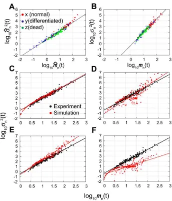
Power-law relation and validity of our model
Here, we focused on the variances of the cell densities in a culture dish. First, we show the relationships between means and variances in the experimental results, which exhibits power-law relation. Second, we extend our model in order to characterize the stochastic properties of the number of cells, and validate the assumption made in the previous sections that parameter values are constant. We also exclude the possibility that a variety of cells with distinct rate constants explain the observed variances in cell densities.
Experimental results exhibit power-law relation. To determine the distribution of cell densities, we calculated the means and the variances at time t; mm^n(t)~PMi~1ni(t)=M, ^
s s2
n(t)~
PM
i~1(ni(t){mm^n(t))
2=(M{1), where n
i denotes the number of cells for n~fx,y,zg, andM denotes the number of data at timet(M~30for our experiments). We found a power-law relationss^2~amm^b whereaand b are constants (Figure 7A). Here, the experimental data shown in Figure 2 were used. We can estimate the probability distribution thatn(t)obeys by calculating the slope b for log10(^ss2)~blog
10(mm^)zlog10(a). For example,
when the distribution ofn(t) has a Poisson distribution, we have the slope b~1, and when the distribution of n(t) has an exponential distribution, we have the slope b~2. For our experiments, the slope b&1:50 and n(t) obeyed neither Poisson nor exponential distributions. This kind of simple power-law relation with several slopes 0:70vbv3:08 is usually observed from microorganisms to animals [21,22], and it is suggested thatb
is an ‘index of aggregation’ describing an intrinsic property of the organisms from near-regular (b?0), through random (b~1) to
highly aggregated (b??). Also, the slope b usually converges within the range 1 to 2, reflecting the balance between birth, death, immigration, and emigration rates [23]. In PC12 cells, immigration and emigration are small on culture dishes because of the slow migration speed compared with the observation time. Thus the slope b&1:50 can reflect the balance between birth, death, and differentiation in our experiment.
Although these results were deduced simply from sample means and unbiased variances, our data include many zero values,
ni~0, especially at timet~0because the density of the cells was very small. We omitted zeros from our data, and we hypothesized that the data obeys a lognormal distribution (the validity of this assumption is assessed in the next section). Then the logarithm of the number of cells obey the normal
distributionN(mm~n(t),~ss2
n(t)), where mm~n(t)~
PM
i~1ln(ni(t))
=M,
~ s s2
n(t)~
PM
i~1fln(ni(t)){mm~n(t)g 2
=(M{1). The variable M
(ƒ30) denotes the number of data with non-zero values. Therefore the means and variances of the original data (ni(t)) are
Figure 7. Power-law relationships between means and
vari-ances of cell density.Experimentally observed relationships between
the means and variances had a slope ofb&1:50(A). When the means and variances were calculated on the basis of lognormal distribution, the slope was b&2:34 (B). Simulation results of the relationships between the means and variances with several assumptions of models were compared with experimentally determined results (C–F). (C) Model parameters were constant, and initial conditions had a lognormal distribution (model-1,b&2:34). (D) Model parameters obey truncated normal distribution, and initial conditions were constant (model-2,
b&2:80). (E) Model parameters displayed truncated normal distribu-tions, and the initial conditions displayed lognormal distributions (model-3,b&2:82). (F) Both model parameters and the initial conditions were constant (model-4,b&1:37). The time courses of changes in the densities of cells (cells=mm2) are used for experimental data. Details are
shown in the main text.
mn(t)~exp mm~nz~ss2n=2
,
s2
n(t)~exp 2mm~nzss~2n
e~ss2n{1
: ð1Þ
The plot of log10mn(t) vs log10s2n(t) (Figure 7B) indicates a power-law relation with a slope of b&2:31 for an equation log10 s2n(t)
~blog10ðmn(t)Þzlog10a. In equation (1), we can
predict that the slopebconverges to2for a constant variance of ~
s s2
n(mm~n??). Thus the variance is not constant, but follows an equation ss~n~ðmm~nÞc where c&1=3, which means that the variance of the number of cells increases as the mean number of cells increases.
A stochastic model with constant parameters exhibits the observed power-law relation. Here, we predict the origins of the relationships between means and variances for our experi-ments by constructing a stochastic version of a model for the equation (3) (Models section). Even when the parameters
h~fm,k1,k2,d1,d2g are constant, the cell-fate decision of each cell is stochastic. When we calculate the state transition process for each cell, the number of cells shows a stochastically changing trajectory. We evaluated whether constant parameters are sufficient to explain the observed variances after repeated calculation of these trajectories.
We assumed that the parameters (i-1) were constant, as defined in Table S1, or that (i-2) obeyed a truncated normal distribution, as defined in the Models section. We also assumed that the initial conditions (ii-1) were constant, as defined in Table S1, or (ii-2) obeyed a lognormal distribution. Using these simple assumptions, we made four models: model-1 with assumptions (i-1) and (ii-2), model-2 with assumptions (i-2) and (ii-1), model-3 with assump-tions (i-2) and (ii-2), and model-4 with assumpassump-tions (i-1) and (ii-1). Using model-1, we could successfully achieve a power-law relationship between means mn(t) and variances s2
n(t) with a slope of b&2:34, which was approximately the same as our experimental result (Figure 7C). Other models did not fit our experimental results (Figure 7D–F). Furthermore, although the power-law relation with a slope of bw2could not be explained with a simple birth–death process model with a slope b&2 (Models section), it could be explained by our birth–death– differentiation model could, and these results did not depend on the environmental serum conditions. Thus, a stochastic model-1 corresponds to the experimental results, and the transition rates of it are constant, with the low level of noise that was assumed in the previous sections. We calculated the distribution of the number of cells using model-1 (details are shown in the Models section), and showed that the number of cells in the results of simulations usually followed a lognormal distribution (Figure S5), which supports the assumption that the distribution is lognormal under the initial conditions. The power-law relationship with b&2:31 and log normal distribution were reproduced robustly in simulations using various parameter values and initial distributions (Fig. S6).
As shown here, a stochastic model with constant parameter values is sufficient to explain the observed power-law relation. Therefore, it is highly probable that a cell fate is decided by stochastic fluctuations in intracellular reactions. However, what decides the rates of fate transitions is still unknown. Interpretations of power-law relations using mathematical models have been performed in several contexts [23,24]. Earlier work [23] suggested that a power-law relation was caused by fluctuating environmental conditions, and that population rate parameters became random variables. They focused on the density effects of populations and assumed that only a parameter of density-dependent coefficient
was random. However, in the present work, our model did not include density effects or other cell–cell interactions, and it was sufficient to consider constant parameter values. Analytical predictions of the power-law relation using some birth–death processes were also suggested previously [24]. The same studies also proposed multi-species models, but did not consider complex state transition model as our model did. Our model suggests that the balance between birth, death, and differentiation affects slopes of power-law relations.
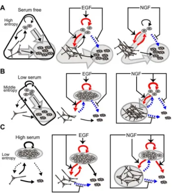
Concluding remarks
We analyzed the time courses of the cell fate decision processes of PC12 cells after the addition of either of the growth factors EGF or NGF under three different environmental serum conditions. The results are summarized in Figure 8A–C. The population of cells became heterogeneous under all of the conditions tested, and high concentrations of serum suppressed the level of heterogeneity. The effects of growth factors depended on the environmental serum conditions, with each of the two growth factors affecting several transition pathways. Using a mathematical model, we could derive the effects of growth factors at the single-cell level. Stochastic single-cell responses to growth factors induced differ-entiation following exposure to EGF and proliferation following exposure to NGF. The use of phase portraits to capture dynamic changes in cell-fate decisions at the population level enabled us to evaluate the effects of serum concentrations and growth factors, and to discover conditions that promote efficient responses to growth factors. Moreover, we found that responses to growth factors were efficient when an appropriate concentration of serum induced a population with a moderate degree of heterogeneity. Finally, we have demonstrated a power-law relation between the means and variances of the local cell density. Stochastic simulation of our model could explain these results and support the validity of our model.
Materials and Methods
Cell culture
Rat PC12 pheochromocytoma cells from the Riken Cell Bank (Tsukuba, Japan) were cultured and maintained at370C,5% CO
2
in Dulbecco’s Modified Eagle Medium (DMEM, containing 4:5g=L glucose) supplemented with 10%horse serum (HS) and 5%fetal bovine serum (FBS). Cells were transferred to a 60-mm culture dish with a density of50{100cells=mm2. One day after
the transfer, the medium was exchanged for DMEM without phenol red and supplemented with three different concentrations of serum: (i)10%HS and5%FBS (high-serum condition), (ii)0:1% HS and0:05%FBS (low-serum condition), and (iii) no serum but supplemented with1%bovine serum albumin (BSA) (serum-free condition). Two days after subculture, cells were treated with8ml of 2:5mg=ml mouse 2.5S nerve growth factor (NGF) (50ng=ml final concentration; Alomone Labs., Jerusalem, Israel), 1:5ml of 100mg=ml recombinant murine epidermal growth factor (EGF) (100ng=mlfinal concentration; Peprotech, London, UK), or10ml of Hank’s balanced salt solution for controls. The medium and the reagents were exchanged every second day.
Cell count
To count the densities of proliferating, differentiated, and dead cells, thirty images of living PC12 cells within thirty areas of0:14 or 0:57mm2 in size were taken for each dish every day after
failure to extend neurites. The differentiated cells were defined by extension of at least one neurite with a fiber length longer than the diameter of the cell body. Dead cells were identified as shrunken or fragmented cell bodies. Examples of the micrograph of the three states of cells are shown in Figure 1A. Four independent experiments were done and the results of a typical experiment from the four are shown in Figures 2 and 7. We used the parameter set estimated from the typical experiment (Table S1) to prepare the data shown in Figure 3, and Figure S5. The average values of estimated parameters or fluxes calculated from the four independent experiments were used to prepare Figures 4, and 5.
Statistical verification methods
In addition to using thep-values determined using at-test, we used effect sizedto compare two groups of data:
d~ mt{mc
ffiffiffiffiffiffiffiffiffiffiffiffiffiffiffiffiffiffiffiffiffiffiffiffiffiffi
(st2zsc2)=2
p , ð2Þ
wheremt denotes a mean for treatment group andmc denotes a mean for control group, andstandscdenote standard deviations for them. This value compares distance of mean values of two groups with mean values of standard deviations of them. When the value of d is large, the difference between two groups is large compared with the standard deviations. Significant values of effect
size d are arbitrarily defined depending on research fields, although the values of d~0:8 for the large effect size, d~0:5 for the middle effect size, and d~0:2 for small effect size are usually used [25].
Analysis of variance was used when more than three population averages were available for comparison. We assumed that there werealevels or conditions of experiments Ai (i~1,2, ,a) and that experiments were repeated ri times in each level Ai. We defined the valuexijasjth data in a levelAi. For example, a level Aidenoted each serum condition, and we repeatedri~4times in each level. The effect sizeg2was defined as follows
g2~SBG Stot,
whereSBGdenoted the between-groups sum of squares, andStot
denoted the total sum of squares:
SBG~X a
i~1 ri
P
jxij ri
{
P
i
P
jxij n
2
,
Stot~X a
i~1
Xri
j~1 xij{
P
i
P
jxij n
2
,
wherendenoted the total number of experiments. The significant effect size g2 was also arbitrarily defined, but the values of
g2~0:14for the large effect size,g2~0:059for the middle effect
size, andg2~0:01 for small effect size were the typically used
criteria, as in the effect sized[25].
Models
State transition model. To estimate the mean transition rates between the cell states, we generated a mathematical model that describes processes that decide cell fates. In this model, we assumed that (i) each cell independently determines cell fates with no cell–cell interaction, (ii) cells do not proliferate when they are differentiated, and (iii) de-differentiation occurs. The second assumption is based on reports indicating that upon treatment with NGF, cells appeared to stop dividing and the number of surviving cells was saturated [11–13,15,18].
dx
dt ~ (m{k1{d1)xzk2y, dy
dt ~ k1x{(k2zd2)y, dz
dt ~ d1xzd2y,
8
> <
> :
ð3Þ
where x, y, and z denote the mean densities (cells/mm2) of proliferating, differentiated, and dead cells, respectively. The parameters m§0,k1§0 and k2§0 denote the proliferation, differentiation, and de-differentiation rates (1=day), respectively. The parametersd1§0and d2§0denote the death rates of the proliferating and differentiated cells (1=day), respectively. Using the limited number of experimental dataD~fXt,Yt,Ztgwheret
denotes the days after stimulation (t~0,1, ,N), we estimated the parameter values in equation (3) applying Bayesian inference to our model (Materials and methods). A typical example of the parameter values from the four independent experimental datasets are shown in Table S1. Time courses of experimental and simulation results are shown in Figure 2. The model successfully estimated the parameters that describe the experimental results.
Figure 8. Responses to growth factors. Responses to growth
factors depended on the use of no (A), low (B), and high (C) serum conditions. Under control conditions, the black thick lines denote the increase of parameter values affected by serum-containing conditions compared with the serum-free condition, and the black dotted lines denote the decrease of the same parameter values. Under each serum condition, the red thick lines denote the increase of parameter values affected by growth factors, and the blue dotted lines denote the decrease of the same parameter values. Arrows and hammer-head arrows of epidermal growth factor (EGF) and nerve growth factor (NGF) denote increase or decrease of parameter values compared with the control conditions, respectively. Gray circles and arrows indicate the population-level cell fate in each conditions.
Analytical solution of a state transition model in a phase space. The velocitiesxx_ andyy_do not depend onz, and we can simplify equations (3) to linear differential equations:
_ x x _ y y ~ m
{k1{d1 k2
k1 {k2{d2
x
y
uuu_~Au: ð4Þ
The eigenvaluesl1andl2, and corresponding eigenvectorsu1and u2of a vectorAprovide an analytical solution of equation (4):
u(t)~c1u1exp(l1t)zc2u2exp(l2t), ð5Þ
wherec1andc2are constants depending on initial conditionsx(0) andy(0). A solutionz(t)can be calculated using the equations (3) and (5). In particular, we can write down the solutions as follows:
x(t)~ 1
2k1 c1(c3{c4)exp c3{c4
2 t
zc2(c3zc4)exp c3zc4 2 t
n o
,
y(t)~c1exp c3{c4 2 t
zc2exp c3zc4 2 t
,
z(t)~
c1 d1 k1z
2d2 c3{c4
exp c3{c4 2 t
zc2 d1 k1z
2d2 c3zc4
exp c3zc4 2 t
zc5, ð6Þ
wherec1,c2,c3,c4, andc5denote
c1~{k1c4{1x(0)zc3c4
{1z1
2 y(0),
c2~k1c4{1x(0){c3c4
{1{1
2 y(0),
c3~m{k1zk2{d1zd2,
c4~
ffiffiffiffiffiffiffiffiffiffiffiffiffiffiffiffiffiffiffiffiffiffiffiffiffiffiffiffiffiffiffiffiffiffiffiffiffiffiffiffiffiffiffiffiffiffiffiffiffiffiffiffiffiffiffiffiffiffiffiffiffiffiffiffiffiffiffiffiffiffiffiffiffiffiffiffiffiffiffiffiffiffiffiffiffiffiffiffiffiffiffiffiffiffiffiffiffiffiffiffiffiffiffiffiffiffiffiffiffiffiffiffiffiffi (m{k1{k2{d1{d2)2{4(d1(d2zk2)zd2(k1{m){k2m)
q
,
c5~z(0){c1 d1 k1z
2d2 c3{c4
{c2 d1 k1z
2d2 c3zc4
:
The solutions of equation (5) are categorized into several types depending on the geometrical features of trajectories around the critical point (x,y)~(0,0) [26]. The dynamics of the number of cells are plotted on a phase space. For linear differential equations, we can simply classify the patterns of solutions depending on the parameter values of equations. When all parameters m,k1,k2,d1, and d2 are constrained to be positive, as in the case of our model, the types of solutions are limited. In our model parameters, the solutions of the characteristic equations have two eigenvalues, and the property of the critical point is a stable node or an unstable saddle. Whereas the former means that a population of cells extincts asymptotically, the latter means that it increases infinitely. Here we define the parameters p~l1zl2, q~l1l2, and D, with D denoting a discriminant of a
characteristic equation of A. Our observation that D was always §0 suggests that the critical point is not a center or
spiral. We found that the critical point was either (i) an asymptotically stable node (pv0 and qw0), or (ii) a saddle point (qv0). Then the vector u is constrained to have limited trajectories.
In our model, the parameter values are always nonnegative. Therefore, the number of cells converges asymptotically to the following equation, with a long time limit [27],
x(t) y(t)
~n0 vx vy
exp(lt), ð7Þ
where n0 denotes an arbitrary initial condition, the Malthus coefficientlis calculated from the equationl~max(l1,l2), and
l1 and l2 are eigenvalues of A in equation (4). The
corresponding eigenvector is(vx,vy)tr. Whenlw0, the number of total surviving cells increases, but whenlv0, it decreases to the origin.
Normalized response rates in the phase space. The rates of responses to external signals compared with a control condition were defined in one of three ways: (i) the Malthusian parameter, (ii) the initial response speeds, or (iii) the time average of response speeds. The Malthusian parameterl~max(l1,l2), wherel1and
l2 are two eigenvalues for our linear model, and the asymptotic
response rateslRwhich are normalized for a control condition are defined as
lEGF=CTL~l
EGF{lCTL
DlCTLD ,
lNGF=CTL~l
NGF{lCTL
DlCTLD
ð8Þ
where lEGF (lNGF) denotes the eigenvalues in the presence of growth factors EGF (NGF), andlCTLdenotes those in the absence of growth factors. The initial response speeds are
Jx(0) Jy(0) Jz(0) 0 B @ 1 C A~
dx(t)=dt dy(t)=dt dz(t)=dt
0 B @ 1 C A
t~0
: ð9Þ
Then, the normalized response speeds are
JEGF=CTL
n ~
JEGF
n (0){JnCTL(0)
DJCTL
n (0)D
,
JNGF=CTL
n ~
JNGF
n (0){JnCTL(0)
DJCTL
n (0)D
,
ð10Þ
wherenis a variablex,y, orz, andJCTL
n (0),JnEGF(0), andJnNGF(0) denote the net fluxes of the number of cells at timet~0in the presence or absence of either EGF or NGF. The time averages of response speeds are
Jx Jy Jz 0 B @ 1 C A~ 1 T ÐT 0 Jx(t)dt 1
T
ÐT
0 Jy(t)dt 1
T
ÐT 0 Jz(t)dt
0 B B @ 1 C C A
, ð11Þ
Jn EGF=CTL
~Jn EGF
{Jn CTL
Jn CTL ,
Jn NGF=CTL
~Jn NGF
{Jn CTL
Jn CTL ,
ð12Þ
wheren is a variablex,y, or z. Also,Jn CTL
, Jn EGF
, and Jn NGF
denote the time averages of the net fluxes of the number of cells at a range of time0vtvT in the presence or absence of EGF or NGF.
Parameter estimation for a deterministic model. To estimate parameter values for our three-state model, we applied Bayesian inference to our experimental data. In addition to the differential equations (3), we assumed that the experimental data of the numbers of three-state cells, Xt, Yt, and Zt, satisfy the observation equations as follows:
Xt ~ axtzgx, Yt ~ aytzgy, Zt ~ aztzgz,
8
> <
> :
ð13Þ
where a(mm{2) is a constant which exchanges the unit of the
average density for that of the average number of cells in a microscope image. The variables t~0, 1, 2, ,N denote the observation time (day), and the parameters gi (i~x,y,z) denote time-independent observation noise that satisfies an identically independent normal probability density function, gi&N(0,si). The likelihood of reproducing the experimental data
D~fXt,Yt,Ztg (t~0, 1, 2, ,N), consisting of 3(Nz1) inde-pendently distributed data points with a set of parameters
h~fm,k1,k2,d1,d2gis defined as:
L(D,h)~f(Djh)~
P
N
t~0 1
ffiffiffiffiffiffiffiffiffiffiffiffiffiffiffiffiffiffiffiffi
2ps2 xs2ys2z
q exp
0
B
@ {
Xt{xt(h) ð Þ2
2s2 x
"
zðYt{yt(h)Þ 2
2s2 y
zðZt{zt(h)Þ 2
2s2 z
!#!
,
ð14Þ
wherext(h),yt(h), andzt(h)are predicted from equations (3) with parametershand initial conditionsx0,y0, andz0. We sought to estimate a set of parameters h, gi, and initial conditions that maximize the above likelihood function L. However, we only applied Bayesian inference to parametersh. We directly estimated the initial conditions from our experimental data, which did not affect estimation ofh. Also, we arbitrarily defined the observation noise gi for which we could attain a sufficiently large value of likelihood L. In our experiments, values of gi (the standard deviationssiwhich ranges from5to30) were able to adequately explain our experimental data.
The posterior probability density function p(hDD) obeys the following equation based on the Bayes’ theorem
p(hDD)~f(DDh)p(h)
p(D) ~
f(DDh)p(h)
Ð
f(DDh)p(h)dh ð15Þ
!f(DDh)p(h), ð16Þ
where p(h) denotes the prior probability density function and
p(D)~Ðf(DDh)p(h)dhdenotes the normalization constant or the marginal likelihood. A sample from the parameter posterior can be obtained using Markov Chain Monte Carlo (MCMC) sampling. Here we used the Metropolis–Hasting algorithm to produce samples from a distribution p(hDD). We assumed the gamma distribution as the prior distribution of p(h), because all model parameters should have non-negative values based on biological requirements. The parametershindependently obey the gamma distribution as follows
hi&G(a,b)~
ha{1 i
C(a)baexp({hi=b), ð17Þ
whereCdenotes the gamma function andhiis an each component of h. In our experimental results, possible ranges of parameters include zero and we seta~1andb~3, where values ofbat least 10times larger did not definitely affect the values estimated with our method. Smaller values of both a and b narrow the distribution, and in general, estimates become biased. Therefore, we used these values to search for parameters in a broad distribution. The candidate parametershare generated using the random walk chain of a normal random number ehi with the variances2
hi:
hi~h(it)zehi, ehi&N(0,s2hi)
whereh(t) denotes a previously selected parameter set. Here we assume that the proposal distribution is symmetric
q(hiDh(it))~ ffiffiffiffiffiffiffiffiffiffiffi1 2ps2
hi
q exp {
(h(it){hi)2 2s2
hi
" #
~q(h(it)Dhi):
Therefore, the acceptance rate of candidate parameters is
a(hiDhi(t))~min 1,p(h
iDD)
p(h(it)DD)
" #
~min 1, f(DDh
i)p(hi) f(DDh(it))p(h(it))
" #
:
To estimate an optimal parameter set, we applied simulated annealing to our data set. Thus the acceptance rate can be modified to
a(hiDhi(t))~min 1, f(DDh
i)p(hi) f(DDh(it))p(h(it))
!1=T(s) 2
4
3
5,
where we assumed that the functionT(s)(s~0,1,2,. . .,smax) which is called the temperature gradually decreases (setting T~1recovers Metropolis sampling) with the following four steps
T(s)~
max½(Ti,1{Tf,1) Tn
h Tn
hzsn
zTf,1,Tm (0ƒsvs1) :step (1)
Tm (s1ƒsvs2) :step (2)
max½(Ti,2{Tf,2) Tnh Tn
hz(s{s2)n
zTf,2,Tf(s2ƒsvs3) :step (3)
Tf (s3ƒsvsmax):step (4)
For a constant time steps~scand a temperatureT(sc), the MCMC chain was repeatedly applied for a fixed sampling numbert~tmax. In the initial step (1), we intended to sample a wide range of parameter space, and cool down the initial high temperatureTi,1~10to the final
oneTm~1to recover Metropolis sampling. A value ofTi,1at least10
times larger did not affect the estimation of the parameter values. For a while, the metropolis sampling was performed in a second step (2) to converge the posterior parameters with distributionp(hDD). In the next step (3), we further decreased the temperatureT(s)fromTi,2~1
to Tf~0:01 in order to estimate a mode of p(hDD). Finally, we repeated sampling with a constant temperatureTf~0:01in the last step (4). In selecting the last temperatureTf, we checked the likelihood valuesL(D,h)in step (4) gradually decreasing the value ofTf. When the likelihood value was saturated, we stopped decreasing the temperature and obtained a value of Tf~0:01. In our estimation procedures, we used the following values tmax~10000, s1~100,
s2~200, s3~300, and smax~500. To determine a suitable parameter set for our experimental results, we used the likelihood value at a temperature T(s); f(DDh,T(s)). When the likelihood becomes maximum in a constant temperatureT(sc), we selected a parameter set h(sc) as the best for that temperature. Then we averaged over parameter setsh(s)in step (4), and defined them as the estimated parameters
hi~
X
smax
s~smin
hi(s)
0
@
1
A=ðsmax{sminÞ, ð18Þ
wheresmin satisfiess3vsminvsmax and we set smin~400 for our experiments. We monitored the selected parameter values for each steps, and confirmed that these numbers of steps (s1{smax) were sufficient to cause the distributions of the parameter values to converge. We evaluated the dependency of the estimation ofh(s)on the initial parameter valuesh(0), the initial temperaturesTi,1, and the
value ofb in a gamma distribution (Figure S7). In our estimation methods, at least10times large values ofbandTi,1, and four orders of
different initial parameter values did not affect estimation of parameter values.
A stochastic version of a state transition model. Here, we seek to make a stochastic model. A scheme of cell fate decision processes is as follows
sx?2sxProliferation rate: m
sx?syDifferentiation rate: k1
sx?szCell death rate: d1
sy?sxDe-differentiation rate: k2
sy?szCell death rate: d2
wheresx,sy, andszdenote states of each cell. All events are first order processes, and rate constants for differential equations can be applied directly to these reaction schemes. We calculated this scheme using the Gillespie algorithm with absorbing boundary conditions at x~y~0 [28], and derived means mn(t) and variancess2
n(t) introduced in equation (1). Here, we can assume several possibilities for (i) the distributions that the parameter values obey, and (ii) the initial conditions x0, y0, and z0 of the densities of cells. For the parameter values, we assume that (i-1) the parameters are constant as defined in Table S1, or (i-2) the parameters obey a truncated normal distribution with the probability density function of
f(x;mparam,sparam,0,?)~
w((x{mparam)=sparam)=sparam
W(?){W({mparam=sparam) (x§0), 0 (xv0),
(
ð19Þ
wheremparam(orsparam) is one of parameter valuesm,k1,k2,d1, d2, w(:) denotes the probability density function of a standard normal distribution N(0,1), and W(:) denotes the distribution function of it. For the initial conditions, we assume that (ii-1) the initial conditions are constant as defined in Table S1, or (ii-2) the initial conditionsx0,y0, andz0obey a lognormal distribution log N(minit,s2
init)with
minit~ln m 2
ffiffiffiffiffiffiffiffiffiffiffiffiffiffiffi
m2zs2 p
,
s2init~ln s 2
m2z1
,
ð20Þ
wherem~s~x0,y0, orz0.
Lognormal distributions (Figure S5) were calculated from simulation results of model-1 at day 5, and involved 10000 samples using parameter values in the high serum condition+ EGF and NGF. In addition, we used100-times larger values for the initial conditions in this figure than in Figure 7, and converted the values from the number of cells to the cell density. For each figure, distributions from simulations were fitted to a normal distribution N(mdata,s2
data); mdata~(
PM
i~1ln(ni))=M and
s2 data~(
PM
i~1fln(ni){mdatag 2)=(
M{1), where ni denotes the simulated non-zero density values of cells at day5andMƒ10000. Analytical solution of birth–death process. When we define the number of cells at timetasN(t), and the probability as
Pn(t)~PfN(t)~ng, the birth–death processes are described by
dP0(t)=dt~lDP1(t), ð21Þ
dPn(t)=dt~{(lBzlD)nPn(t)zlB(n{1)Pn{1(t)
zlD(nz1)Pnz1(t),
ð22Þ
where the birth rate from the sateN(t)~nislB,n~nlB, and the death rate from the sateN(t)~nislD,n~nlD. The steady state probability is obtained by
lim
t??dP0(t)=dt ~0,
lim
t?? dPn(t)=dt ~0:
If the birth and death rates are lBvlD, the number of cells converges to limt??N(t)~0 and the probability becomes limt?? P0(t)~1, which suggests extinction of a population. If the birth and death rates are lDvlB, the number of cells converges to limt??N(t)~? and the probabilities are limt?? P0(t)~P0v1 and limt?? Pi(t)~0 (i~1,2,3, ); this suggests an infinite increase of a population with probability 1{P0. The means and the variances of the number of cells M(t)~P?n~1 nPn(t) and
V(t)~P?n~1 n2Pn(t){(P?
n~1nPn(t)) 2