Abstract Real convergence in per capita output and growth in Eurozone: a time-series approach

(1)

Work Project presented as part of the requirements for the Award of a Master’s Degree in

Economics from the NOVA School of Business and Economics.

REAL CONVERGENCE IN PER CAPITA OUTPUT AND GROWTH IN EUROZONE: A TIME-SERIES APPROACH

GONÇALO ANTÓNIO NOGUEIRA DE SOUSA PINTO (Student number 720)

A Project carried out on the Master in Economics Program, under the supervision of Professor Paulo M.M. Rodrigues

(2)

Abstract

Real convergence in per capita output and growth in Eurozone: a time-series approach

The real convergence hypothesis has spurred a myriad of empirical tests and approaches in the economic literature. This Work Project intends to test for real output and growth convergence in all N(N-1)/2 possible pairs of output and output growth gaps of 14 Eurozone countries. This paper follows a time-series approach, as it tests for the presence of unit roots and persistence changes in the above mentioned pairs of output gaps, as well as for the existence of growth convergence with autoregressive models. Overall, significantly greater evidence has been found to support growth convergence rather than output convergence in our sample.

JEL classification: C32, E01, E23, O4, O11

(3)

I. Introduction

With the inception of the European Economic Community (EEC) with the Treaty of Rome in 1957, we witnessed in the second half of the 20th century a significant deepening of commercial, social and institutional relations between European countries. In the aftermath of World War II, many European regions were still deprived of resources and communities struggled to make ends meet. In such a context and alongside the European project, the European Social Fund (ESF) was created in 1958, subsequently followed by the European Regional Development Fund (ERDF) in 1975. Both these funds had at their cornerstone the idea of providing funds to regions in difficulty in order to equip them with the means to converge with the richer regions in Europe. Such funds started gaining a great deal of momentum with the accession of Greece, Spain and Portugal to ensure that their level of output would increase and be more on par with the remaining members of the EEC. Since then, every entrant in the now European Union has had the chance to benefit from such structural funds, a powerful tool for convergence across Europe.

(4)

WP is the strong evidence we found against long-run convergence in our sample and, in contrast, the significant evidence favouring the existence of real per capita output growth convergence. The rest of the paper is structured as follows: section II presents the literature review; section III develops the existing notions of output convergence; section IV contains the data and its description; section V presents our methodology and the empirical results whereas section VI concludes.

II. Literature Review

The Solow-Swan model (1956) predicts that similar economies, in terms of production technology and economic agents’ preferences but with different rates of capital intensity, will converge to the same steady-state, thus shrinking over time their output differences. However, researchers came across incongruences between this model and empirical evidence and, also, this model does not predict secular per capita output growth, unless it is set via exogenous technological progress. Thus, it has spurred the development of other models that could explain long-term growth in economies using an endogenous growth approach, by including the source of growth in its intrinsic dynamics. Notable work under this approach was done primarily by Lucas (1988) and Romer (1986).

(5)

considered in his paper presents a framework of analysis with the inclusion of non-diminishing returns to capital in the aggregate economy due to positive knowledge externalities between economic agents. Unlike the Arrow (1962) version of this model, Romer’s version has

explosive growth associated to it, as the aggregate production function exhibits increasing returns to scale. Economies with more capital intensity will produce higher growth rates than economies with less capital intensity and, therefore, this model does not present any theoretical grounds for the notion of convergence between countries.

Following Durlauf, Johnson and Temple (2004), we have as main empirical approaches to the convergence phenomenon the cross-country approach and the time-series approach. On the one hand, the cross-country approach sets out to determine if a country is undertaking β -convergence or not, and relies on the neoclassical model of growth with or without extensions.

Thus, it is tested if β<0 in the following regression as presented by Durlauf (2003):

𝑔𝑖 = 𝑦𝑖,0𝛽 + 𝑋𝑖𝛿 + 𝑍𝑖𝛾 + 𝜀𝑖 (1)

where _𝑔_𝑖 is the real per capita output of a given country i on a time interval, _𝑦_𝑖,0is the per capita

output on the outset of the series, _𝑋_𝑖 refers to a set of additional regressors implied by the neoclassical model, _𝑍_𝑖represents a group of regressors which are proxy for variables deemed relevant in new economic growth theories and _𝜀_𝑖 is the error term.

(6)

the regressors and endogeneity and, lastly, variable measurement errors and the lack of power of such tests against non-convergent alternatives based on new growth theories or multiple equilibria models, like the Azariadis-Drazen (1990) model.

(7)

correct tool to properly assess the existence of convergence when the series exhibit long memory, that is, when the shocks in the series fade away at a hyperbolic and not a typical geometric rate. As for notable results in the literature under this approach we have Bernard and Durlauf (1995) who turns to 15 advanced economies using Maddison data on GDP between 1900 and 1989, finding little evidence for convergence and Hobijn and Franses (2000), who also do not find significant evidence of convergence across 112 countries taken from the Penn World Table for the period 1960-1989 using a clustering algorithm for club convergence identification.

Finally, let us now focus on literature concerning the European case. Constantini and Lupi (2005) offer an approach to convergence in Europe based on independent and dependent panel unit root tests for 15 European countries using two subsamples with Germany as the benchmark country: the first between 1950 and 1976 and the second between 1977 and 2003. The results present significant evidence for convergence in the first period but not in the second. Moreover, we have a cluster analysis done by Monfort et al. (2013) using econometric techniques based on factor analysis which provide evidence on divergence in EU-14 countries globally speaking but, at the same time, detected the existence of 2 convergence clubs. Additionally, according to Gligorić (2014) and using a pair-wise panel unit root approach for a crisis and a non-crisis subsample with quarterly data spanning from 1995 until 2013, catching-up processes are prevalent in Europe while long-run convergence is restricted to 3 convergence clubs. Reza and Zahra (2008) study real convergence in the ten 2004 European Union entrants with the usage of different unit root tests finding evidence of absolute convergence and catching-up processes with the EU-25 average and the EU-15 per capita output. Finally,

statistical evidence of β-convergence is found in the work done by Cuaresma et al. (2013) who

(8)

III. Definition of Convergence

In the first place, let us compare the notion of β-convergence with σ-convergence. As

defined by Durlauf, Johnson and Temple (2004), β-convergence is the first measure of convergence used in modern literature and is associated to cross-country approaches for testing the convergence hypothesis. It corresponds to the catching-up effect, on which a less capital-intensive country benefits from the technology diffusion made by the countries in the technological frontier and further benefits from having higher marginal products of capital. These two factors induce higher growth regimes in such countries. On the other hand, σ

-convergence refers to the cross-country dispersion of output across countries. If this dispersion

(9)

Yet, let us now focus on the statistical definitions. According to Durlauf (2003), convergence can be defined as the _lim

𝑘→+∞𝜇(𝑔𝑖,𝑡+𝑘|𝑆𝑖,𝑡, 𝜃, 𝜌) not depending on Si,t , being µ(.) a

probabilistic measure, Si,t the human and physical capital endowments and θ and ρ the

technology and preferences of the economy, respectively. This definition is furthered with two additional definitions by Bernard and Durlauf (1996). Their Definition 1 is stated as follows:

𝐸(𝑦𝑖,𝑡+𝑇− 𝑦𝑗,𝑡+𝑇|ℑ𝑡) < 𝑦𝑖,𝑡− 𝑦𝑗,𝑡 (2)

where _𝑦_𝑖,𝑡 and _𝑦_𝑗,𝑡 are the logs of per capita output of country i and j, respectively and _ℑ_𝑡

represents all the information at time t. This means that output growth is not influenced by the initial endowments of human and physical capital of an economy, leading us to infer that the long-term reduction of output level discrepancies between economies is expected.

On the other hand, these authors also define convergence as the long-term equalisation of log per capita output for both countries at time t, as it is stated by the following equation:

lim

𝑘→+∞𝐸(𝑦𝑖,𝑡+𝑘− 𝑦𝑗,𝑡+𝑘| ℑ𝑡) = 0 (3)

Still, for our main analysis, we are going to use the definition of long-run convergence of Pesaran (2004). His definition of pair-wise convergence is a probabilistic one, and less restrictive than the one postulated by Bernard and Durlauf (1996), presented here as follows:

lim

𝑠→∞𝑃𝑟{|𝑦𝑖,𝑡+𝑠− 𝑦𝑗,𝑡+𝑠| < 𝐶|ℑ𝑡} > 0 (4)

(10)

economies to have different microeconomic fundamentals such as endowments, saving rates and population growth rates. An output differential series having a zero sample mean is not a necessary condition for the existence of convergence according to this definition.

IV. Data

The data retrieved for our analysis corresponds to annual observations of real per capita Gross Domestic Product (GDP) in Geary-Khamis dollars (international 1990 US dollars) of 14 Eurozone countries spanning from 1950 to 2015. The data was later logarithmised and used to calculate the N(N-1)/2 combinations of output differentials between the 14 countries, i.e., a total of 91 output differentials. This data was retrieved from The Conference Board Total Economy DatabaseTM_{as of May 2015.}

V. Methodology and empirical analysis

Following the definition of convergence proposed by Pesaran (2004) described earlier, we are going to represent the output gap series having as basis the model suggested by Lee, Pesaran and Smith (1996):

𝑦𝑖𝑡− 𝑦𝑗𝑡 = (𝑐𝑖 − 𝑐𝑗) + (𝑔𝑖− 𝑔𝑗)𝑡 + (𝑢𝑖𝑡− 𝑢𝑗𝑡) + 𝜀𝑖𝑗𝑡 (5)

where _(𝑐_𝑖 _{− 𝑐}_𝑗₎ is a fixed effect dependent on the country pairs respective initial conditions,

(𝑔𝑖− 𝑔𝑗)𝑡 is a deterministic time trend related to the countries technological growth rates,

(𝑢𝑖𝑡− 𝑢𝑗𝑡) is an idiosyncratic stochastic component of technology that follows an

autoregressive process and _𝜀_𝑖𝑗𝑡_{~𝑖𝑖𝑑(0, 𝜎}2₎_.

(11)

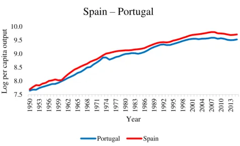
information criterion (BIC) and a significance level of 5%. In Table A.1, in the Appendix, we can find the results of such testing on our data. With these tests, alongside trend significance tests covered ahead, we come to the conclusion that long-run convergence is not happening in Eurozone as a whole, but we detect 7 long-run convergence cases which roughly represent 8% of all series. They are, namely, Belgium – Austria, Finland – Austria, Spain – Belgium, Germany – France, Italy – France, Netherlands – Germany and, lastly, Spain – Portugal. These were the only cases where the ADF tests revealed stationarity and we could not detect a deterministic component in the respective series.

For robustness and to complement these findings, we turn to the work developed by Harvey et al. (2006) on persistence change testing and their modified versions of ratio-based statistics developed by Kim (2000, 2002) and Busetti and Taylor (2004) as presented in the Appendix, model B.1. We apply to these series the Vogelsang-based approach variant of the modified mean, exponential and maximum score statistics to test for I(0) to I(1) persistence changes and their reciprocals for I(1) to I(0) persistence changes, i.e. MSm min, MEm min, MXm

min and MSmRmin, MEmRmin, MXmRmin, respectively. According to the authors, these are the

test-statistics which produce less size distortion and, at the same time, possess the most size-adjusted power. It should be noted that these tests dismiss 15% of the observations: the former in the beginning and their reciprocals in the end of the series and that we will only consider one persistence change due to our relatively small sample. Finally, these test statistics are compared to the critical values presented in the above mentioned paper correspondent for a sample size of T=100 and a nominal significance level of 5% (α=5%).

(12)

𝑦𝑖,𝑡 − 𝑦𝑗,𝑡= 𝛼𝑖𝑗+ 𝛽𝑖𝑗𝑡 + ∑𝑝𝑖=1𝛾𝑖𝑗(𝑦𝑖,𝑡−𝑖− 𝑦𝑗,𝑡−𝑖) + 𝜀𝑡 (6)

(13)

Figure 1: Log of per capita output in Spain and Portugal To be noted that the number of long-run convergence cases is heterogeneous amongst the countries in our sample. Whereas Italy and the Netherlands display 4 cases of long-run convergence each, Cyprus, Greece, Ireland and Malta, peripheral countries of the EMU, do not present one single case of long-run convergence case. As a final note, most persistence change break dates can be found in the time period between 1956 and 1966, a period of time coincidental with the outset of the deepening of market integration of Western European Countries within the EEC and also within the European Free Trade Association (EFTA).

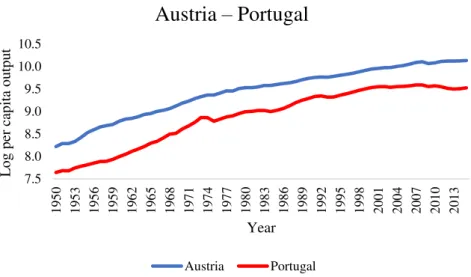
Nevertheless, we should take into account that, in our data, not rejecting the null hypothesis of nonstationarity does not necessarily mean that a pair of countries is on a divergence path. In fact, due to the catching-up effects of a country in relation to the benchmark, the output differential series might display nonstationarity and we can still infer favourably to the convergence hypothesis between these two countries, though without the statistical backing we find for the stationary cases.

7.5 8.0 8.5 9.0 9.5 10.0 19 50 19 53 19 56 19 59 19 62 19 65 19 68 19 71 19 74 19 77 19 80 19 83 19 86 19 89 19 92 19 95 19 98 20 01 20 04 20 07 20 10 20 13 L og p er ca pita ou tp ut Year

Spain

–

Portugal

(14)

Figure 2: Log of per capita output of Austria and Portugal Take, for instance, the case of Austria and Portugal. The output gap between these two countries is nonstationary. Thus, in the light of our empirical analysis we would argue that these two nations are not converging when it is not the case. Actually, the nonstationarity detected in the series has more to do with the catching-up dynamics followed by Portugal (interrupted in 2009 with the Great Recession and subsequent Sovereign Debt Crisis) than with output divergence.

Lastly, we follow once again Pesaran (2004) and test for convergence in our sample in terms of output growth rates. Hence, considering g as a country’s growth rate, we test: 𝐻𝑔𝑐: 𝑔𝑖𝑗 = 𝑔𝑖 − 𝑔𝑗 = 0 for all i and j. According to the above mentioned author, we can test

such hypothesis by testing the statistical significance of the short and long-run intercept in the following regression:

𝑔𝑖𝑡− 𝑔𝑗𝑡 = 𝑔𝑖𝑗 + ∑𝑝_𝑠=1𝑖𝑗 𝜑𝑖𝑗(𝑔𝑖,𝑡−𝑠− 𝑔𝑗,𝑡−𝑠) + 𝑣𝑖𝑗𝑡 (7)

which is an _{𝐴𝑅(𝑝}_𝑖𝑗₎ model where _𝑝_𝑖𝑗is determined using the BIC. For the long-run intercept,

HAC Newey-West estimation was used with the lags being automatically selected based on the

7.5 8.0 8.5 9.0 9.5 10.0 10.5 19 50 19 53 19 56 19 59 19 62 19 65 19 68 19 71 19 74 19 77 19 80 19 83 19 86 19 89 19 92 19 95 19 98 20 01 20 04 20 07 20 10 20 13 L og p er ca pita ou tp ut Year

Austria

–

Portugal

(15)

BIC. The short-run intercept is _𝑔_𝑖𝑗 whereas the long-run intercept corresponds to the derived

long run equilibrium of the AR model:

𝑔𝑖𝑗∗ = _1−∑𝑔𝑖𝑗_𝜑

𝑖𝑗 𝜌𝑖𝑗 𝑠=1

. ₍₈₎

The summary of the results can be found in the Appendix, in Table A.3. For illustration, in the first line of table A.3, Austria is our benchmark country and we detect short and long-run output growth convergence for all other countries in our sample with the exception of France

and Netherlands for α=5% and Malta for α=10% We happen to find more evidence of growth

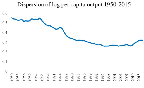
convergence in our sample than for output convergence, being Malta the only nation in which growth convergence does not appear to be prevalent, showing somewhat mixed results. In reality, we came across 82 cases of short-run convergence and 81 cases of long-run growth convergence for α=5% (roughly 90% and 89% of all series, respectively), capturing most cases of countries which, according to our previous tests, were not converging in terms of output. In fact, when taking a look at the dispersion, measured by the standard deviation of the output growth rates of the 14 Eurozone countries of our sample (see Appendix Figure A.6), we can see a significant reduction as of 1978-1979, stabilising within a small window of values. However, one can detect a slight increase in such dispersion between 2008 and 2012, the period of time corresponding to the Great Recession and subsequent Sovereign Debt Crisis which had a significant impact in the Greek, Portuguese, Irish and Cypriot economies. This overall dispersion reduction seems to be coincidental with the introduction of the European Exchange Rate Mechanism (ERM), which produced exchange rate stabilisation of member-state currencies with the European Currency Unit (ECU) and, therefore, progressive harmonisation of member-state monetary policies in preparation for the implementation of the single currency

(16)

VI. Conclusions

(17)

VII. References

Andrews, Donald. 1993. "Tests for Parameter Instability and Structural Change with Unknown Change Point." Econometrica, 61(4), 821-56.

Andrews, Donald and Werner Ploberger. 1994. "Optimal Tests When a Nuisance Parameter Is Present Only under the Alternative." Econometrica, 62(6), 1383-414.

Arrow, Kenneth J. 1962. "The Economic Implications of Learning by Doing." The Review of

Economic Studies, 29(3), 155-73.

Azariadis, Costas and Allan Drazen. 1990. "Threshold Externalities in Economic Development." The Quarterly Journal of Economics, 105(2), 501-26.

Barro, Robert J. 1991. "Economic Growth in a Cross Section of Countries." The Quarterly

Journal of Economics, 106(2), 407-43.

Barro, Robert J. and Xavier Sala-i-Martin. 1992. "Convergence." Journal of Political

Economy, 100(2), 223-51.

Bart, Hobijn and Franses Philip Hans. 2000. "Asymptotically Perfect and Relative Convergence of Productivity." Journal of Applied Econometrics, 15(1), 59-81.

Baumol, William J. 1986. "Productivity Growth, Convergence, and Welfare: What the Long-Run Data Show." American Economic Review, 76(5), 1072-85.

Bernard, Andrew B. and Steven N. Durlauf. 1995. "Convergence in International Output."

Journal of Applied Econometrics, 10(2), 97-108.

____. 1996. "Interpreting Tests of the Convergence Hypothesis." Journal of Econometrics,

71(1–2), 161-73.

Busetti, Fabio and AM Robert Taylor. 2004. "Tests of Stationarity against a Change in Persistence." Journal of Econometrics, 123(1), 33-66.

(18)

Costantini, Mauro and Claudio Lupi. 2005. "Stochastic Convergence among European Economies." Economics Bulletin, 3(38), 1-17.

Crespo Cuaresma, Jesus; Miroslava Havettová and Martin Lábaj. 2013. "Income Convergence Prospects in Europe: Assessing the Role of Human Capital Dynamics."

Economic Systems, 37(4), 493-507.

Dowrick, Steve and Duc-Tho Nguyen. 1989. "Oecd Comparative Economic Growth 1950-85: Catch-up and Convergence." American Economic Review, 79(5), 1010-30.

Durlauf, S.N. and University of Wisconsin--Madison. Social Systems Research Institute. 2003. The Convergence Hypothesis after 10 Years. Social Systems Research Institute,

University of Wisconsin.

Durlauf, Steven; Paul Johnson and Jonathan Temple. 2004. "Growth Econometrics," Wisconsin Madison - Social Systems,

Gligorić, Mirjana. 2014. "Paths of Income Convergence between Country Pairs within

Europe." Ekonomski Anali / Economic Annals, 59(201), 123-55.

Hansen, B.E. 1991. "Testing for Structural Change of Unknown Form in Models with Nonstationary Regressors."

Harvey, David I.; Stephen J. Leybourne and A. M. Robert Taylor. 2006. "Modified Tests for a Change in Persistence." Journal of Econometrics, 134(2), 441-69.

Kim, Jae-Young. 2000. "Detection of Change in Persistence of a Linear Time Series."

Journal of Econometrics, 95(1), 97-116.

Kim, Jae-Young; Jorge Belaire-Franch and Rosa Badillo Amador. 2002. "Corrigendum to "Detection of Change in Persistence of a Linear Time Series" [J. Econom. 95 (2000) 97-116]." Journal of Econometrics, 109(2), 389-92.

Lee, K.; M. H. Pesaran and R. Smith. 1996. Growth and Convergence in a Multicountry

(19)

Lucas, Robert E. 1988. "On the Mechanics of Economic Development." Journal of

Monetary Economics, 22(1), 3-42.

Mankiw, N. Gregory; Romer David and N. Weil David. 1990. "A Contribution to the Empirics of Economic Growth," National Bureau of Economic Research, Inc,

Mills, T.C. and K. Patterson. 2009. Palgrave Handbook of Econometrics: Volume 2:

Applied Econometrics. Palgrave Macmillan.

Monfort, Mercedes; Juan Carlos Cuestas and Javier Ordóñez. 2013. "Real Convergence in Europe: A Cluster Analysis." Economic Modelling, 33, 689-94.

Perron, Pierre. 1989. "The Great Crash, the Oil Price Shock, and the Unit Root Hypothesis."

Econometrica, 57(6), 1361-401.

Pesaran, M. H. 2004. "A Pair-Wise Approach to Testing for Output and Growth Convergence," Faculty of Economics, University of Cambridge,

Peter, C. B. Phillips and Perron Pierre. 1986. "Testing for a Unit Root in Time Series Regression," Cowles Foundation for Research in Economics, Yale University,

Peter, C. B. Phillips and Xiao Zhijie. 1998. "A Primer on Unit Root Testing," Cowles Foundation for Research in Economics, Yale University,

Ranjpour, Reza and Zahra Karimi Takanlou. 2008. "Evaluation of the Income

Convergence Hypothesis in Ten New Members of the European Union. A Panel Unit Root Approach." Panoeconomicus, 55(2), 157-66.

Robert, J. Barro and Sala-i-Martin Xavier. 1991. "Convergence across States and Regions." Brookings Papers on Economic Activity, 22(1), 107-82.

____. 1990. "Economic Growth and Convergence across the United States," National Bureau of Economic Research, Inc,

Romer, Paul. 1986. "Increasing Returns and Long-Run Growth." Journal of Political

(20)

Solow, Robert M. 1956. "A Contribution to the Theory of Economic Growth." The Quarterly

Journal of Economics, 70(1), 65-94.

Vogelsang, Timothy. 1998. "Trend Function Hypothesis Testing in the Presence of Serial Correlation." Econometrica, 66(1), 123-48.

VIII. Appendix

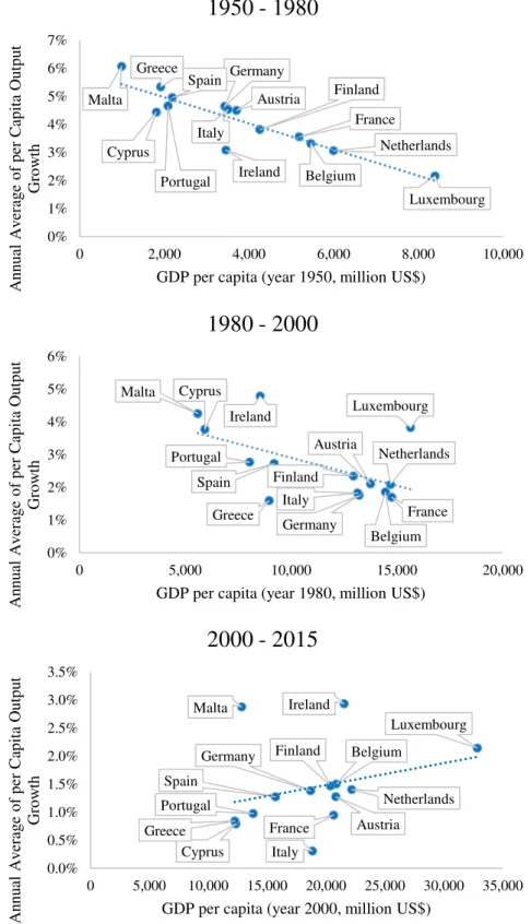
Figure A.1: Output growth vs initial values of GDP per capita

Austria Belgium Cyprus Finland France Germany Greece Ireland Italy Luxembourg Malta Netherlands Portugal Spain 0% 1% 2% 3% 4% 5% 6% 7%

0 2,000 4,000 6,000 8,000 10,000

A nn ual A ver ag e of p er C ap ita Ou tp ut Gr ow th

GDP per capita (year 1950, million US$)

1950 - 1980

Austria Belgium Finland France Germany Greece Ireland Luxembourg Malta Netherlands Portugal Spain 0.5% 1.0% 1.5% 2.0% 2.5% 3.0% 3.5% ag e of p er C ap ita Ou tp ut Gr ow th

2000 - 2015

Austria Belgium Cyprus Finland France Germany Greece Ireland Italy Luxembourg Malta Netherlands Portugal Spain 0% 1% 2% 3% 4% 5% 6%

0 5,000 10,000 15,000 20,000

A nn ual A ver ag e of p er C ap ita Ou tp ut Gr ow th

(21)

Figure A.2: σ-convergence

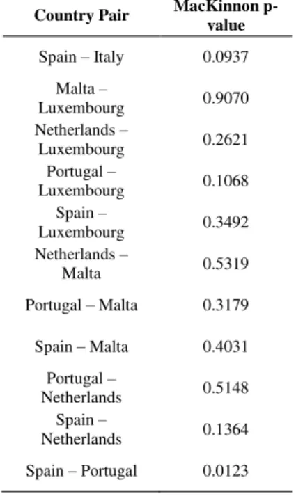
Table A.3: ADF test results and time trend significance test results

Country Pair MacKinnon p-value

Belgium – Austria 0.0001

Cyprus – Austria 0.5492

Finland – Austria 0.0040

France – Austria 0.0011

Germany – Austria 0.0020

Greece – Austria 0.5178

Ireland – Austria 0.4210

Italy – Austria 0.9528 Luxembourg –

Austria 0.0942

Malta – Austria 0.5526

Netherlands –

Austria 0.2488

Portugal – Austria 0.4914

Spain – Austria 0.4774

Cyprus – Belgium 0.5465

Finland – Belgium 0.1393

France – Belgium 0.3295

Germany –

Belgium 0.0144

Greece – Belgium 0.0771

Ireland – Belgium 0.3005

Italy – Belgium 0.2017

Luxembourg –

Belgium 0.6095

Malta – Belgium 0.4371

Netherlands –

Belgium 0.5251

Portugal – Belgium 0.1396

Spain – Belgium 0.0180

Finland – Cyprus 0.4338

France – Cyprus 0.6067

Germany – Cyprus 0.3426

Greece – Cyprus 0.4694

Ireland – Cyprus 0.4744

Italy – Cyprus 0.1533

Luxembourg –

Cyprus 0.2492

Malta – Cyprus 0.4593

Netherlands –

Cyprus 0.7946

Portugal – Cyprus 0.3463

Spain – Cyprus 0.2399

France – Finland 0.0921

Germany – Finland 0.0060

Greece – Finland 0.2055

Ireland – Finland 0.6864

Italy – Finland 0.4825

Luxembourg –

Finland 0.4450

Malta – Finland 0.4846

Netherlands –

Finland 0.1292

Portugal – Finland 0.3244

Spain – Finland 0.2269

Germany – France 0.0004

Greece – France 0.1630

Ireland – France 0.6331

Italy – France 0.0469 Luxembourg –

France 0.3491

Malta – France 0.3151

Netherlands –

France 0.5029

Portugal – France 0.5613 0 0.1 0.2 0.3 0.4 0.5 0.6 19 50 19 53 19 56 19 59 19 62 19 65 19 68 19 71 19 74 19 77 19 80 19 83 19 86 19 89 19 92 19 95 19 98 20 01 20 04 20 07 20 10 20 13

(22)

Spain – France 0.5157

Greece – Germany 0.4874

Ireland – Germany 0.1656

Italy – Germany 0.6539

Luxembourg –

Germany 0.0001

Malta – Germany 0.3568

Netherlands –

Germany 0.0287 Portugal –

Germany 0.4063

Spain – Germany 0.3546

Ireland – Greece 0.8479

Italy – Greece 0.5005

Luxembourg –

Greece 0.5526

Malta – Greece 0.4834

Netherlands –

Greece 0.0501

Portugal – Greece 0.2646

Spain – Greece 0.3332

Italy – Ireland 0.1671

Luxembourg –

Ireland 0.6365

Malta – Ireland 0.5413

Netherlands –

Ireland 0.1343

Portugal – Ireland 0.5983

Spain – Ireland 0.7264

Luxembourg – Italy 0.9176

Malta – Italy 0.2550

Netherlands – Italy 0.3222

Portugal – Italy 0.0120

Spain – Italy 0.0937

Malta –

Luxembourg 0.9070 Netherlands –

Luxembourg 0.2621 Portugal –

Luxembourg 0.1068 Spain –

Luxembourg 0.3492 Netherlands –

Malta 0.5319

Portugal – Malta 0.3179

Spain – Malta 0.4031

Portugal –

Netherlands 0.5148 Spain –

Netherlands 0.1364

Spain – Portugal 0.0123

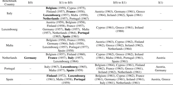
Table A.4: Modified tests for persistence change results summary

Benchmark

Country I(0) I(1) to I(0) I(0) to I(1) I(1)

Austria – BelgiumFrance (1994), Germany (1959), (1975), Finland (1958), Luxembourg (1959)

Cyprus (1962), Greece (1962), Italy (1963), Malta (1963)

Ireland, Netherlands, Portugal, Spain

Belgium –

Austria (1975), France (1963), Germany (1960), Italy (1959), Luxembourg (1958), Malta (1958),

Netherlands (1957)

Cyprus (1962), Finland (1962), Greece (1962), Ireland (1962), Portugal (1964),

Spain (1961) –

Cyprus – Italy (1975)

Austria (1962), Belgium (1962), Finland (1962), France (1962), Germany (1962),

Greece (1962), Ireland (1962), Luxembourg (1961), Malta (1962), Netherlands (1962), Portugal (1961),

Spain (1962)

–

Finland –

Austria (1958), France (1957), Germany (1957), Italy (1957), Luxembourg (1958), Netherlands

(1960), Spain (1972)

Belgium (1962), Cyprus (1962), Greece (1961), Ireland (1964), Malta (1962),

Portugal (1962) –

France –

Austria (1994), Belgium (1963), Finland (1957), Germany (1960),

Italy (1958), Luxembourg (1957), Malta (1958), Netherlands (1957),

Cyprus (1962), Greece (1962), Ireland

(1962), Portugal (1963), Spain (1961) –

Germany Netherlands

Austria (1959), Belgium (1960), Finland (1957), France (1960), Luxembourg (1957), Malta (1964)

(1961), Italy (1961), Spain (1961) Portugal

Greece – –

Austria (1962), Belgium (1962), Cyprus (1962), Finland (1961), France (1962),

Germany (1963), Ireland (1961), Italy (1964), Luxembourg (1961), Malta (1962), Netherlands (1962), Portugal

(1961)

Spain

Ireland – –

Belgium (1962), Cyprus (1962), Finland (1964), France (1962), Germany (1961), Greece (1961), Italy (1962), Luxembourg (1988), Malta (1962), Netherlands (1961),

(23)

Benchmark

Country I(0) I(1) to I(0) I(0) to I(1) I(1)

Italy –

Belgium (1959), Cyprus (1975),

Finland (1957), France (1958),

Luxembourg (1957), Malta (1958),

Netherlands (1957), Portugal (1967)

Austria (1963), Germany (1961), Greece

(1964), Ireland (1962), Spain (1961) –

Luxembourg –

Austria (1959), Belgium (1958), Finland (1958), France (1957), Germany (1957), Italy (1957), Malta (1957), Netherlands (1964), Portugal

(1965), Spain (1961)

(1988) –

Malta –

Belgium (1958), France (1958), Germany (1964), Italy (1958), Luxembourg (1957), Portugal (1977),

Spain (1958)

Austria (1963), Cyprus (1962), Finland (1962), Greece (1962), Ireland (1962),

Netherlands (1964) –

Netherlands Germany

Belgium (1957), Finland (1960),

France (1957), Italy (1957), Luxembourg (1964)

Cyprus (1962), Greece (1962), Ireland (1961), Malta (1964), Portugal (1961),

Spain (1961)

Austria

Portugal – Italy (1967), _{Malta (1977),}Luxembourg_Spain₍₁₉₅₉₎ (1965), Belgium (1964), Cyprus (1961), Finland (1962), France (1963), Greece (1961), Ireland (1962), Netherlands (1961)

Austria, Germany

Spain – Finland(1961), Malta (1958), (1972), LuxembourgPortugal

(1959)

Belgium (1961), Cyprus (1962), France (1961), Germany (1961), Ireland (1961),

Italy (1961), Netherlands (1961)

Austria, Greece

Persistence break dates in parenthesis

Table A.5: Growth Convergence Summary

Benchmark Country

Growth convergence Growth divergence

Short-run Long-run Short-run Long-run

Austria

Belgium, Cyprus, Finland, Germany, Greece, Ireland,

Italy, Luxembourg, Portugal, Spain

France (**), Malta (*), Netherlands

(**)

France (***), Malta (*), Netherlands(**)

Belgium

Austria, Cyprus, Finland, France, Germany, Greece, Ireland, Italy, Luxembourg,

Netherlands, Portugal

Austria, Cyprus, Finland, France, Germany, Greece, Ireland, Italy, Luxembourg,

Netherlands, Portugal

Malta (***), Spain (*) Malta (***), Spain (**)

Cyprus

Austria, Belgium, Finland, France, Germany, Greece, Ireland, Italy, Luxembourg,

Malta, Netherlands, Portugal, Spain

Austria, Belgium, Finland, France, Germany, Greece, Ireland, Italy, Luxembourg,

Finland

Austria, Belgium, Cyprus, France, Germany, Greece, Ireland, Italy, Luxembourg,

Netherlands, Portugal, Spain

Austria, Belgium, Cyprus, France, Germany, Greece, Ireland, Italy, Luxembourg,

Malta (*) Malta (*)

France

Italy, Luxembourg, Netherlands

Belgium, Cyprus, Finland, Greece, Ireland, Italy, Luxembourg, Netherlands

Austria (**), Malta (**), Portugal (*), Spain (**)

Austria (***), Germany (*), Malta (**), Portugal

(*), Spain (**)

Germany

Austria, Belgium, Cyprus, Finland, France, Greece, Ireland, Italy, Luxembourg,

Austria, Belgium, Cyprus, Finland, Greece, Ireland, Italy, Luxembourg, Malta,

Malta (*) France (*)

Greece

Austria, Belgium, Cyprus, Finland, France, Germany, Ireland, Italy, Luxembourg, Netherlands, Portugal,

Spain

Austria, Belgium, Cyprus, Finland, France, Germany, Ireland, Italy, Luxembourg,

Malta(*)

Ireland

Austria, Belgium, Cyprus, Finland, France, Germany, Greece, Italy, Luxembourg,

(24)

Benchmark Country

Growth convergence Growth divergence

Short-run Long-run Short-run Long-run

Italy

Austria, Belgium, Cyprus, Finland, France, Germany,

Greece, Ireland, Luxembourg, Netherlands,

Portugal, Spain

Austria, Belgium, Cyprus, Finland, France, Germany,

Greece, Ireland, Luxembourg, Netherlands,

Portugal, Spain

Malta (**) Malta (**)

Luxembourg

Austria, Belgium, Cyprus, Finland, France, Germany, Greece, Ireland, Italy, Netherlands, Portugal,

Spain

Austria, Belgium, Cyprus, Finland, France, Germany, Greece, Ireland, Italy, Netherlands, Portugal,

Spain

Malta (**) Malta (**)

Malta Cyprus, Germany, Ireland, _{Portugal, Spain} Cyprus, Germany, Greece, _{Ireland, Portugal, Spain}

Austria (*), Belgium (***), Finland (*), France

(**), Greece (*) Italy (**), Luxembourg (**),

Netherlands (**)

Austria (*), Belgium (***), Finland (*), France (**),

Italy (**), Luxembourg (**), Netherlands (**)

Netherlands

Belgium, Cyprus, Finland, France, Germany, Greece, Ireland, Italy, Luxembourg,

Portugal

Belgium, Cyprus, Finland, France, Germany, Greece, Ireland, Italy, Luxembourg

Austria (**), Malta (**), Spain (**)

Austria (**), Malta (**), Portugal (*), Spain (**)

Portugal

Austria, Belgium, Cyprus, Finland, Germany, Greece, Ireland, Italy, Luxembourg, Malta, Netherlands, Spain

Austria, Belgium, Cyprus, Finland, Germany, Greece, Ireland, Italy, Luxembourg,

Malta, Spain

France (*) France (*), Netherlands (*)

Spain

Austria, Cyprus, Finland, Germany, Greece, Ireland, Italy, Luxembourg, Malta,

Portugal

Austria, Cyprus, Finland, Germany, Greece, Ireland, Italy, Luxembourg, Malta,

Portugal

Belgium (*), France (**), Netherlands (**)

Belgium (**), France (**), Netherlands (**)

*** p<0.01, ** p<0.05, * p<0.1

Figure A.3: Dispersion of output growth rates in our sample

0 0.01 0.02 0.03 0.04 0.05 0.06 0.07 0.08 19 51 19 54 19 57 19 60 19 63 19 66 19 69 19 72 19 75 19 78 19 81 19 84 19 87 19 90 19 93 19 96 19 99 20 02 20 05 20 08 20 11 20 14

(25)

B.1: Tests for persistence of output differentials model

To understand how our used persistence change tests work, first we have to take into account the underlying model assumed for such testing. We follow the model presented by Harvey et al. (2006):

𝑦𝑡 = 𝑥𝑡′+ 𝑣𝑡

𝑣𝑡 = 𝜌𝑡𝑣𝑡−1+ 𝜀𝑡, 𝑡 = 1, … , 𝑇; 𝑥𝑜 = 0 (9)

It should be noted that xt corresponds to a set of deterministic variables, 𝑣_𝑡 satisfies the

mild regularity conditions defined by Phillips and Xiao (1998) and the innovation sequence is

assumed to follow a mean zero process that satisfies the familiar α-mixing conditions of Phillips and Perron (1986) with strictly positive and bounded long-run variance _𝜔2_{= lim}

𝑇→∞𝐸(∑ 𝜀𝑇) 2_{. 4}

hypotheses to be tested are presented in the paper:

1. H1: the series is integrated of order 1 (nonstationary) across the sample period and 𝜌_𝑡=

1 − 𝑐/𝑡, _𝑐 equal or greater than zero in order to allow for unit root and local to unit root behaviour in the series.

2. H01: the series changes from I(0) to I(1) at time [𝜏∗𝑇], i.e, 𝜌_𝑡= 𝜌, 𝜌 < 1 for t equal or

smaller than _[𝜏∗_𝑇] and _𝜌_𝑡 _{= 1 − 𝑐/𝑡} for_{𝑡 > [𝜏}∗_𝑇]. The change point proportion τ*_is assumed to be an unknown point in _{Λ = [𝜏}_𝑙_{, 𝜏}_𝑢_], an interval in (0,1) symmetric around 0.5;

3. H10: yt is changing from I(1) to I(0) at time [𝜏∗𝑇];

4. H0: the series is stationary throughout the sample period.

Therefore, Kim (2000), Kim et al. (2002) and Busetti and Taylor (2004) develop tests for the constant I(0) data-generating process against the I(0) – I(1) change (H01) based on the

following ratio statistic:

𝐾[𝜏𝑇]=(𝑇−[𝜏𝑇])

−2_∑ _(∑𝑡 _𝜐̃_𝑖𝜏₎ 𝑖=[𝜏𝑇]+1 𝑇

𝑡=[𝜏𝑇]+1 2

[𝜏𝑇]−2_∑ _(∑𝑡 _𝜐̂_𝑖𝜏 𝑖=1 )2 [𝜏𝑇]

𝑡=1

₍₁₀₎

(26)

(2002) and Busetti and Taylor (2004) take into account three statistics based on the sequence of statistics _{{𝐾(𝜏), 𝜏 𝜖 Λ}}, where _{Λ = [𝜏}_𝑙_{, 𝜏}_𝑢]. These are:

𝑀𝑆 = 𝑇−1_∑[𝜏𝑢] _{𝐾(𝑠/𝑇)}

𝑠=[𝜏𝑙] (11)

𝑀𝐸 = 𝑙𝑛 {{𝑇∗−1∑𝑠=[𝜏[𝜏𝑢]𝑙]exp [₂1𝐾(𝑠/𝑇)]} (12)

𝑀𝑋 =_{𝑠 𝜖 {[𝜏}𝑚𝑎𝑥_𝑙_{], … , [𝜏}_𝑢_{} 𝐾(𝑠/𝑇)} ₍₁₃₎

where _𝑇_∗ _{= [𝜏}_𝑢_{] − [𝜏}_𝑙_{] + 1}. MS, ME and MX correspond to Hansen’s (1991) mean score statistic, Andrews and Ploberger’s (1994) mean-exponential statistic and Andrews’ (1993) maximum statistic. To test H0 against the H10 hypothesis, Busetti and Taylor (2004) propose

tests based on the reciprocals of Kt, i.e. MSR, MER and MXR. To test for an unknown direction

of change, they propose MSM, MEM, MXM which are the pairwise maximum statistics.

To modify these statistics, the authors use the Vogelsang (1998) approach:

𝑀𝑆𝑚= exp(−𝑏𝐽1,𝑇) 𝑀𝑆 (14)

𝑀𝐸𝑚 = exp(−𝑏𝐽1,𝑇) 𝑀𝐸 (15)

𝑀𝑋𝑚 = exp(−𝑏𝐽1,𝑇) 𝑀𝑋 (16)

where b is determined by simulation, assuming _{𝛼̅ = 0}, for a particular level of significance

and _𝐽_1,𝑇 is T-1 the Wald statistic for testing the joint hypothesis 𝛾_𝑘+1 =. . . = 𝛾₉ in the

following regression:

𝑦𝑡 = 𝑥′𝑡𝛽 + ∑9𝑖=𝑘+1𝛾𝑖𝑡𝑖 + 𝑒𝑟𝑟𝑜𝑟, 𝑡 = 1, … , 𝑇 (17)