Abstract
This paper proposes a novel variable-length beam element that takes into account the effect of beam spinning. This is the first such beam element of variable length based on the absolute nodal coordinate formulation. In addition to the position and slope vec-tors, the angles of rotation around the element axis of cross sections that contain two nodes are introduced into the element coordinates to describe the spinning of an assumed Euler–Bernoulli beam with circular cross section. The material coordinates of the two nodes are also included in the arbitrary Lagrangian–Eulerian description used for previous element to describe the varying element length caused by mass transportation at the boundaries. The proposed element facilitates convenient and effective numerical modeling of the dynamics of a circular-cross-section beam with transportation boundaries and that is spinning. Numerical examples demonstrate that the proposed element can describe the dynamic behavior of a circular-cross-section beam effectively. In the field of engineering, this novel element could be used in the dynamic analysis of drill stems, the slender workpiece of a cylindrical shaft during the turn-ing process, and the lead screw in a ball screw mechanism.
Keywords
Beam, circular cross section, absolute nodal coordinate formulation, arbitrary Lagrangian–Eulerian description, variable-length beam-shaft element, spinning.
A Variable-Length Beam Element
Incorporating the Effect of Spinning
1 INTRODUCTION
In the late 1990s, Shabana (1996) proposed a new method for modeling the dynamics of flexible multi-body systems. Known as the absolute nodal coordinate formulation (ANCF), this method is based on the finite element method (Bonet and Wood, 1997; Khan et al., 2016) and continuum mechanics (Shabana, 2012; Asemi et al., 2014). Unlike conventional formulations (e.g., large rota-tion vector and floating frame of reference formularota-tions) that use both global and local reference
Shuai Yang a, * Zongquan Deng a Jing Sun b Yang Zhao c Shengyuan Jiang a
a State Key Laboratory of Robotics and
System, Harbin Institute of Technology, Harbin, China
b Beijing Spacecrafts Manufacturing
Factory, China Academy of Space Technology, Beijing, China
c School of Astronautics, Harbin
Insti-tute of Technology, Harbin, China
* Corresponding author: email: [email protected]
http://dx.doi.org/10.1590/1679-78253894
frames, the ANCF uses only a global reference frame. A position vector and its gradients defined in the global frame are selected as the generalized coordinates of each node. This ensures that no re-striction is imposed on the amount of rotation within the finite element, thereby describing the mo-tion of a flexible multi-body system more exactly (Shabana, 1997). As such, the ANCF has received extensive attention since it first appeared and has been developed considerably over the past 20 years. Various types of ANCF-based finite elements have been developed to apply this method to the dynamic analysis of flexible multi-body systems including structures of beams (Shabana, 1997; Sugiyama and Suda, 2007), plates (Dmitrochenko and Pogorelov, 2003; Dufva and Shabana, 2005), shells (Mikkola and Shabana, 2003), and three-dimensional (3D) solids (Kubler et al., 2003).
In the research area of ANCF-based beam elements, Shabana (1997) first developed a beam el-ement based on the assumption of planar strain. Omar et al. (2001) then developed a two-dimensional (2D) shear-deformable beam element. Following on from 2D beam elements, Shabana and Yakoub (2001, 2001) developed a 3D beam element that uses the position vector and its three gradients as node coordinates. This element relaxes the rigid-section assumption of classical beam theory. It describes cross-sectional deformation using two position gradients, making it a more gen-eral model than the Timoshenko beam model. Unfortunately, this element is disadvantageous for the dynamic analysis of very slender beam structures because of the locking problem. Dombrowski (2002) developed a beam element based on the Euler–Bernoulli beam assumption. This element is better at describing slender beams because the number of coordinates of each node is reduced from 12 to 7 compared with Shabana’s 3D beam element. This element can be used to resolve problems with torsional beam dynamics because Tait–Brian angles are used to describe the cross-sectional spinning; however, the mass matrix of the element is no longer constant. Besides, the singularity introduced by Tait–Brian angles prevents this element from being used to describe arbitrary spatial motions. Gerstmayr and Shabana (2006) developed a 3D cable element that abandons the rotational angles of Dombrowski’s beam element and exhibits advantages in the dynamics of 3D slender beams for which the effect of spinning can be neglected.
and therefore fails to describe the bending deformation. Hence, it is applicable to the dynamic mod-eling of cables that sustain only tension.
All of the aforementioned variable-length tether/beam elements neglect beam spinning; there-fore, they cannot be applied to certain engineering problems such as the dynamic modeling and simulation of drill stems in the drilling process. In this work, we develop a novel variable-length ANCF-based beam element that includes the effect of spinning. Our intention is to resolve the dy-namics of a circular-cross-section (CCS) beam of variable length for which the effect of spinning cannot be neglected. We refer to this novel element as a variable-length beam-shaft element (VLBSE) to reflect the introduction of both bending and spinning effects.
In addition to the position and slope vectors, we introduce the angles of rotation around the el-ement axis of cross sections that contain two nodes into the generalized coordinates of this elel-ement to describe the spinning motion. This is done on the assumptions of an Euler–Bernoulli beam and a CCS. The material coordinates of the nodes are also included in the ALE description used for pre-vious element to describe the variation of element length caused by mass transportation at the boundaries. The rotational angles and material coordinates appear as unknowns in the dynamic equations along with the position and slope vectors. Hence, the VLBSE provides a convenient and effective numerical modeling method for the dynamics of CCS beams with either simple or complex transportation boundaries and for which spinning cannot be neglected.
The VLBSE can be used in the dynamic analyses of (i) the drill stem of a planetary soil-drilling sampler in a deep-space exploration mission (Tian et al., 2012; Deng et al., 2014; Yang et al., 2014), (ii) the slender workpiece of a cylinder shaft in a turning process (Lv et al., 2015; Han et al., 2012), and (iii) slender rods in linear motion elements (Katz, 2001; Huang and Wang, 2014).
In the present work on the VLBSE, we begin by introducing the variables that are used to de-scribe the motion of the element, the generalized coordinates of the element, and the corresponding shape-function matrix. We then address the axial strain, bending curvature, and change rate of rotational angle of cross section, all of which describe the deformation of the element. The mass matrix and generalized force matrix of the element are given by calculating the virtual work of the inertial and active forces. Based on these matrices, a mathematical description of the dynamical model of a CCS beam that has been discretized into elements is obtained according to the general equation of dynamics. Finally, the novel element is verified by three series of typical dynamical problems concerning an axially moving beam/string, a torsion shaft with one end fixed and the other end free, and a rotating shaft subjected to an axially moving and rotating load.
2 MOTION AND DEFORMATION OF THE ELEMENT
The following assumptions are made about the beam before establishing the VLBSE.
(a) The beam cross sections are rigid and remain perpendicular to the beam axis during defor-mation because of the slenderness of the beam.
(b) Any bending-induced rotational inertia effects relative to the neutral axis of the beam cross sections are neglected.
Assumption (c) is consistent with the Euler–Bernoulli beam assumption because a non-CCS would distort if the beam were subjected to torsion.
The motion of an element can be described by two features: translation of an arbitrary point on the element axis, and rotation of the corresponding cross section. Translation of a point on the ele-ment axis can be described by the position vector r of the point. Rotation of a cross section can be described using only the third Tait–Brian angle instead of the direction cosine matrix of the element local reference frame with respect to the global reference frame in the general case with the Euler– Bernoulli beam assumption according to Dombrowski’s work (Dombrowski, 2002). This angle is written as θ, the physical meaning of which is the rotational angle of the cross section around the element axis.
Hence, the motion of the VLBSE is described by four variables that can be expressed as a gen-eralized position vector of an arbitrary point on the element axis:
η rT θ T T
r1 r2 r3 θ . (1)
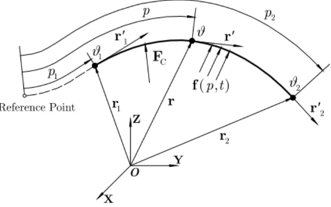
A schematic of the VLBSE is shown in Figure 1. In addition to r and θ, r' is the slope vector of the arbitrary point on the element axis. The derivative is with respect to p, i.e., r' = ∂r/∂p, where p
is the material coordinate of the point, which is the arc length along the unstrained beam from the reference point. Terms r1, r'1, θ1, p1, r2,r'2, θ2, and p2 are the corresponding parameters of the two nodes. Function f(p,t) is the distributed external load per unit length on the element, and FC is the concentrated force on the element. The concentrated torque T is not marked in the figure.
Figure 1: Schematic of the VLBSE.
A control volume for the element can be expressed as [ ( ), ( )]p t p t1 2 using an interval
representa-tion. In the ALE framework, both p1 and p2 are time-dependent functions, which means that there is mass transportation across both element boundaries and that an element can slide and stretch arbitrarily on the beam. However, if p1 and p2 remain constant, there is no mass transportation across the element boundaries; the VLBSE becomes a fixed-length beam-shaft element in the La-grangian framework. The material coordinate p can be normalized into a local coordinate s that satisfies
r
' r
θ
p
1
' r
1
r
1 θ 1 p
2
r
2
' r
2 θ 2 p
C
F
( , )p t f
Reference Point
O
X
1 2
2 1 ( ) ( ) ( ) ( )
p p t p t
s
p t p t
2 -
-=
- . (2)
From equation (2), the local coordinates of the first and second nodes are −1 and 1, respectively. The length of the unstrained element is
2 1
( )= ( )- ( )
e
L t p t p t . (3)
Of the four components of the generalized position vector, the first three corresponding to the position vector are interpolated using third order polynomials to ensure continuity of the position and slope vectors at the nodes. The position vector can then be written as
' '
r =N1 1r +N2r +1 N3 2r +N4r2, (4)
where
=
N1 1 s- 1 2 2 +s
4 , =
L
N2 e s-1 2 s+1
8 ,
=
N3 1 s+ 1 2 2 -s
4 , =
L
N4 e s+1 2 s- 1
8 .
(5)
The fourth component of the generalized position vector corresponding to the rotational angle is interpolated using a linear polynomial:
θ=H1 1θ +H2 2θ , (6)
where
H1 1 1 -s2
=
, H2 1
1+s2
=
. (7)Equations (4) and (6) can be unified as
1 1 ' '
r rr I I 0 I I 0
0 0 0 0 r
r
N N N N θ
H H
θ
θ
1 1 1 3 3 2 3 3 3 3 3 3 4 3 3 3 1
1 3 1 3 1 1 3 1 3 2 2
2 2
= , (8)
which can be simplified to
e1e 1 2 e e1 e2 e1 e1 e2 e2 e2
( ) ( ) ( )
qS q S S S q S q
q
p t, = p p t p t, , t = = +
To partition the matrix Se, two submatrices
1 1
et
et1 et2
S = S S = N1 3 3I N2 3 3I 03 N3 3 3I N4 3 3I 03 , (10) er
er1 er2
S = S S = 01 3 01 3 H1 01 3 01 3 H2 , (11)
are defined to represent the first three lines and the fourth line, respectively, leading to the follow-ing equations:
et
e et e er e
er
θ= S = =
S r S q S q
S . (12)
The first and second derivatives of the generalized position vector with respect to time (i.e., the generalized velocity and acceleration, respectively) can be written as
η=Sq, (13)
p
η=Sq+η , (14)
where
e e
e1 e e2 e
1 2
S S
S = S q S q
p p (15)
is the shape-function matrix of the element,
e1 1 e2 2 ' 1 ' 2
q= qT p qT p T = r1T rT1 θ1 p r2T rT2 θ2 p T (16)
represents the generalized coordinates of the element, and
2 2 2
e e e e e
p 1 2 e 1 1 2 2 e
1 2 1 1 2 2
S S S S S
η p p q p p p p q
p p p p p p
2 2
2 2
= 2 + + + 2 + (17)
is an additional generalized acceleration due to mass transportation across the element boundaries. This term vanishes if there is no mass transportation, in which case both p1 and p2 are constants.
Matrix S is partitioned in the same way as Se (i.e., two submatrices St and Sr represent the first three lines and the fourth line, respectively), leading to the following equations:
t
t r
r
S
S = r = S q = S q
S θ , (18)
et et
t et1 e et2 e
1 2
S S
S = S q S q
p p , (19)
er er
r er1 e er2 e
1 2
S S
S = S q S q
p p . (20)
Because the VLBSE is part of the beam, the deformation description of the beam also applies to the element. Due to the Euler–Bernoulli beam assumption, only one the nine components of the Green–Lagrange strain tensor is nonzero, which is the axial strain, besides, the bending curvature of the beam axis and the change rate of the rotational angle of the cross section are also taken into account to describe the beam deformation. These three components are given by
T
' ' r r
1
= - 1
2
, (21)
' ''
'
r r
r
κ= ×3 , (22)
'
θ θ
p
= = , (23)
where r" is the second derivative of r with respect to p, i.e., r''= 2r p2 . The axial strain
measures the extension of the beam axis, the bending curvature measures the change of orientation of the tangent vector of beam axis, and the change rate of the rotational angle measures the twist of beam. The detailed expressions of r', r" and θ' can be written as:
et et
e e
' = = =
S S
r
r q s q
p p p s , (24)
et et
e e
'' = = =
S S
r
r q q
2
2 2
2
2 2 2
s
p p p s , (25)
er er
e e
' = = =
θ s
θ
p p p s
S S
q q . (26)
3 MASS MATRIX AND GENERALIZED FORCE MATRIX OF THE ELEMENT
The virtual work due to inertial force arises from both translational acceleration of material particles on the element axis and rotational angular acceleration of the cross sections:
2 1
i
r r
q M q Qp T T
p
W = -ρA dp+ θ -ρIθ dp =- ele + p , (27) where ρ, A, and I are material density, area, and polar moment of inertia, respectively, of the ele-ment cross section. Terms Mele and Qp are the mass matrix and the matrix of the additional gener-alized inertial force caused by mass transportation, respectively. Under the assumption of uniform material density, these can be written as
1
I 0M S S
0 T -A p ρ ds I s
1 3 3 3
1 ele
1 3
= , (28)
1 p
I 0Q S η
0 T -A p ρ ds I s
1 3 3 3
1 p
1 3
= . (29)
A block diagonal matrix appears in the integrands of these two matrices, which is unlike exist-ing elements in the literature. The virtual work of viscoelastic forces arises from tension, bendexist-ing, and torsion of the element:
s s sκ s
W = W + W + W , (30)
where Ws, Wsκ, and Wsφ are the virtual-work contributions of tension, bending, and torsion, respectively. Specifically,
2 1
p -s p T T T - s pW - EA c dp - EA c ds
s
p
- EA c ds
-s 1 1 1 1 = + = + = + = q q
q q Q
q
, (31)
where E and c are the elasticity modulus and damping coefficient, respectively. Term Qs is the
generalized viscoelastic force matrix resulting from the tension of the element:
T -s pEA c ds s
1 1
= +
Q
q , (32)
where,
T
' '
=r r , (33)
t ' = = =
r r S
r d d q
and T ' ' r r
q= q , (35)
et e'
S q
r r
q q q
2 2
= =
p p . (36)
Similarly,
2 1
p T
sκ p sκ
W =- EJ κ+cκ κdp=- q Q , (37)
2 1
p
T s p s
W =- GI +c dp=- q Q , (38)
where J is the moment of inertia of the element cross section and G is the shear modulus. Terms
Qsκ and Qsφ are the generalized viscoelastic force matrices of element resulting from bending and torsion, respectively:
T -sκ pEJ κ cκ ds s
κ
1 1 = + Qq , (39)
T -s pGI c ds
s
1 1
= +
Q
q . (40)
The virtual work of the viscoelastic forces can then be written as
T T T T
s s sκ s s
W =- q Q - q Q - q Q =- q Q , (41)
where Qs is the generalized viscoelastic force matrix and can be written as
s = s + sκ+ s
Q Q Q Q . (42)
In particular, when beam torsion or bending is negligible, Qsφ or Qsκ can be omitted accordingly.
The virtual work of a distributed external load can be written as
2 1
p T T
f p
W = r fdp= q Qf, (43)
where Qf is the generalized external force matrix of the distributed external load:
t T -p ds s 1 1 f =
Q S f . (44)
t
T
F = C
Q S F , (45)
r
QT =ST
T
. (46)The total virtual work of an element can then be obtained as
q M q Q
ele= T ele + ele
W - , (47)
where Qele is the generalized force matrix of the element:
s
ele= p+ - f - F- T
Q Q Q Q Q Q . (48)
To resolve the dynamics of a CCS beam with mass transportation, we divide the beam into sev-eral VLBSEs that are connected by nodes. Suppose that the beam consists of N elements; therefore, there are N+1 nodes. The generalized coordinates of the beam are
1 2
' ' '
1T 1T θ1 p 2T 2T θ2 p … N+1T N+1T θN+1 pN+1
T=
q r r r r r r . (49)
In general, these coordinates are not completely independent, for example: in the case that the beam is connected at node i with a fixed point C in the inertial reference frame by means of a spherical joint, the constraint equation is given as
i
r =rC, (50)
in another case that all of the elements of the beam are of equal length, the constraint equations are given as
1 N
p p p
N N
i N+1
- + 1 - 1
=
i
+i
i 2,3,...,N
= . (51)More constraint equations of different joints are given by García-Vallejo et al. (2003). These constraint equations can be expressed uniformly in the form of an algebraic equation as
C q,t = . 0 (52)
By introducing a Lagrange multiplier λ, the dynamical equation of the beam can be obtained as
+ + T =
q
Mq Q C λ 0, (53)
where M and Q are the mass matrix and generalized force matrix, respectively, of the beam. These derive from Mele and Qele of each element, with Cq being the Jacobian matrix of the constraint.
4 NUMERICAL EXAMPLES AND DISCUSSION
The VLBSE is verified in this section. The first example is used to show that this element retains the ability of the VLBE to resolve the dynamics of a CCS beam with mass transportation in the case without spinning. The second example is used to demonstrate the ability of this novel element to resolve purely torsional dynamics. Synthetic verification of the VLBSE is carried out in the third example. Finally, potential engineering applications of the VLBSE are discussed.
4.1 Free Flexural Vibration Analysis of an Axially Moving Beam
When a beam moves continuously along its own axis, as shown in Figure 2, its transverse vibra-tional characteristics are affected significantly by the global axial motion. In Figure 2, OXZ repre-sents the inertial reference frame, and x is the coordinate in the X direction. The target object in this example is the beam section between the two supports. The beam is in continuous motion; hence, the deflection of cross section should be seen as a function of the field coordinate x and time
t in the framework of Eulerian description (Liu et al., 2011).
Figure 2: Axially moving beam.
Suppose that the beam cross section is uniform and circular. The length of the beam section be-tween the supports is l, its cross-sectional area is A, its material density is ρ, its flexural stiffness is
EJ, and its deflection is expressed as w(x,t). The beam travels at a constant speed υ0 in the X direc-tion under the acdirec-tion of tension F. The dynamic equation of free flexural vibration can be written as (Liu, 2012; Wickert and Mote, 1990)
2
w w w w
ρA ρAv EJ F ρAv
t x t x x
2 4 2
2
0 0
2 +
2
+ 4 - - 2 = 0. (54)To study the natural frequency characteristics more conveniently, the flexural stiffness of the beam can be neglected. In that case, the axially moving beam degenerates to an axially moving string, and the dynamic equation can be simplified to
2
w w w
ρA ρAv ρAv F
t x t x
2 2
2
0 0
2 +
2
+ - 2 = 0. (55)The first-order natural frequency of the free transverse vibration of the string can be written as
F F
w x
X Z
P
0
P
l
O
2
f c v
lc
2
1 0
1
=
-2 , (56)
where c = F (ρA) is the axial propagation speed of the string’s transverse vibration.
Conventional ANCF elements in the Lagrangian framework are not suitable for modeling the beam section that flows between the supports in this example, because their target object is the continuum in initial configuration throughout. If the target object is the continuum in a certain fixed region in space, the ALE description degenerates into the Eulerian description. Therefore, the transverse vibrational characteristics of an axially moving beam/string are studied in the following using Hong’s VLBE (Hong and Ren, 2011; Hong et al., 2011) and the VLBSE proposed in this pa-per, which are both established in the ALE framework.
The geometric, material, and kinematic parameters of the axially moving beam/string are given in Table 1, where r is the cross-sectional radius.
Parameter l r ρ E F v0
Value 1 m 0.005 m 2700 kg/m³ 70 GPa 1000 N 40 m/s
Table 1: Simulation parameters of an axially moving beam/string.
(1) ANCF solutions of free transverse vibration of an axially moving string
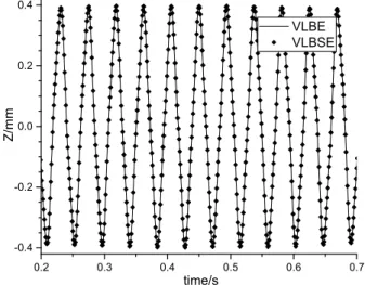
The string section between the two supports is divided into four elements of equal length. The string begins vibrating freely because of the initial transverse velocities of three intermediary nodes. Transverse displacements of the material point halfway between the supports are compared in Fig-ure 3 for two types of element.
Figure 3: Comparison of transverse displacements of the material point halfway between supports.
The transverse-displacement–time curves obtained using the two different elements are nearly coincident. According to equation (56), the first-order natural frequency of the transverse vibration of the string should be 22.6857 Hz; the numerical solutions give 22.6723 Hz (VLBSE) and
0.2 0.3 0.4 0.5 0.6 0.7
-0.4 -0.2 0.0 0.2 0.4
Z/
m
m
time/s
22.6786 Hz (VLBE) with relative errors that are both less than 0.1%. These results demonstrate that, in the dynamic analysis of a CCS beam subjected to only tension, the VLBSE can describe the continuum dynamics effectively.
(2) ANCF solutions of free flexural vibration of an axially moving beam
Mesh generation for a beam section between two supports is the same as that for a string sec-tion, but now bending is taken into account in the dynamic equations. The beam begins vibrating freely because of the initial transverse velocities of three intermediary nodes. The deflections of the material point halfway between the supports are compared in Figure 4 for two types of element.
Figure 4: Comparison of deflections of the material point halfway between supports.
The deflection–time curves obtained using the two different elements are nearly coincident. The numerical solutions for the first-order natural frequency of flexural vibration of the beam are 32.2097 Hz (VLBSE) and 32.2425 Hz (VLBE), with a relative error of approximately 0.1%. Fur-thermore, the first-order natural frequency of transverse vibration of an axially moving beam is clearly greater than that of an axially moving string as the result of flexural stiffness. In the case described by the simulation parameters given in Table 1, the natural frequency increases from 22.7 Hz to 32.2 Hz. The above results demonstrate that, in the dynamic analysis of a CCS beam subjected to both tension and bending, the VLBSE can describe the continuum dynamics effectively.
From the above analysis of the free transverse vibration of an axially moving beam/string, we see that the VLBSE retains the ability of the VLBE to resolve the dynamics of a CCS beam with mass transportation but without spinning. In fact, the VLBSE degenerates to the VLBE if the rota-tional angles θ1 and θ2 both remain zero.
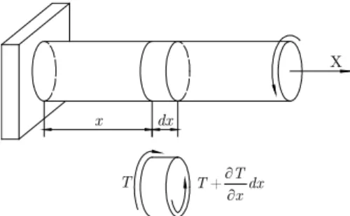
4.2 Free Torsional Vibration Analysis of a Cylindrical Shaft
The model for free torsional vibration of a cylindrical shaft is shown in Figure 5. The length of the cylindrical shaft is l, the material density is ρ, and the shear modulus is G. The X axis is set to
co-0.5 0.6 0.7 0.8 0.9
-0.4 -0.2 0.0 0.2 0.4
Z/
mm
time/s
incide with the central axis of the shaft, with x the coordinate in the X direction. The rotational angle of the cross section is expressed as θ(x,t), and the torque acting on the cross section is T(x,t).
Figure 5: Model for free torsional vibration of a cylindrical shaft.
This torsional vibration model can be expressed mathematically as a one-dimensional wave equation (Gatti and Ferrari, 2003):
θ θ
c
t x
2 2
2
2 = 2 , (57)
where c= G ρ is the axial propagation speed of the torsional vibration. The torsional natural frequencies fi of a shaft that is fixed at x = 0 and free at x = l are
=2 - 1 = 1,2,... 42 -1
4
i
i c i G
f i
l l ρ (58)
The VLBSE in the ALE framework degenerates into a conventional element in the Lagrangian framework if the material coordinates of both nodes are invariant. Therefore, it applies to resolve problems of torsional vibration of the shaft in this example. Free torsional vibration of the shaft are analyzed below using the ANCF. The shaft is divided into different numbers (from 1 to 10) of VLBSEs of equal length. The geometric and material parameters of the shaft are given in Table 2, where r is the cross-sectional radius, and E and μare the elastic modulus and Poisson’s ratio, re-spectively, of the material.
Parameter l r ρ E μ
Value 1 m 0.005 m 2700 kg/m³ 70 GPa 0.3
Table 2: Simulation parameters of a cylindrical shaft.
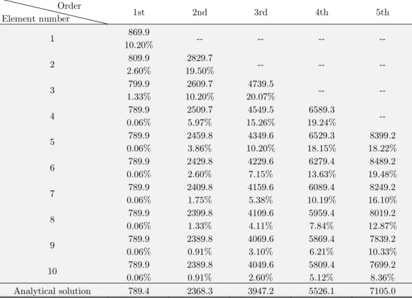
Table 3 gives the numerical solutions and their relative errors for the first five orders of torsion-al naturtorsion-al frequencies of the cylindrictorsion-al shaft for different numbers of elements; “--” means that the corresponding order of natural frequencies does not exist.
x
T dx
X
T
T dx
x
Order
Element number 1st 2nd 3rd 4th 5th
1 869.9 -- -- -- --
10.20%
2 809.9 2829.7 -- -- --
2.60% 19.50%
3 799.9 2609.7 4739.5 -- --
1.33% 10.20% 20.07%
4 789.9 2509.7 4549.5 6589.3 --
0.06% 5.97% 15.26% 19.24%
5 789.9 2459.8 4349.6 6529.3 8399.2
0.06% 3.86% 10.20% 18.15% 18.22%
6 789.9 2429.8 4229.6 6279.4 8489.2
0.06% 2.60% 7.15% 13.63% 19.48%
7 789.9 2409.8 4159.6 6089.4 8249.2
0.06% 1.75% 5.38% 10.19% 16.10%
8 789.9 2399.8 4109.6 5959.4 8019.2
0.06% 1.33% 4.11% 7.84% 12.87%
9 789.9 2389.8 4069.6 5869.4 7839.2
0.06% 0.91% 3.10% 6.21% 10.33%
10 789.9 2389.8 4049.6 5809.4 7699.2
0.06% 0.91% 2.60% 5.12% 8.36%
Analytical solution 789.4 2368.3 3947.2 5526.1 7105.0
Table 3: Numerical solutions and their relative errors for torsional natural frequencies (Hz) of a shaft.
Table 3 reveals a decrease in shaft torsional stiffness with element number, in that the numeri-cally determined torsional natural frequencies decrease accordingly and converge toward the analyt-ical solutions. The relative error of the first-order torsional natural frequency drops below 1% at element number 4. The relative error of the second-order torsional natural frequency drops below 1% at element number 9. Eventually, the relative error of even the fifth-order torsional natural frequen-cy drops to 8.36% when the shaft is divided into 10 elements.
This example demonstrates that in the dynamic analysis of a CCS beam subjected to only tor-sion, the VLBSE can describe the continuum dynamics effectively if the mesh is fine enough.
4.3 Dynamic Response of a Spinning Shaft Subjected to an Axially Moving and Rotating Load
which are expressed as U1 and U2, respectively, as shown in Figure 6(b). The deflections U1 and U2
and their derivatives with respect to time are all zero initially.
(a) spinning shaft subjected to an axially
moving and rotating load (b) bending description of a spinning shaft
Figure 6: Dynamic model of a spinning shaft subjected to an axially moving and rotating load.
Using complex notation, the dynamic equation of the spinning shaft (Katz, 2001; Katz et al., 1988) can be written as
4 2
U U U UEJ ρA -ρJ - Ω P z,t
z t z t z t
4 3
4 + 2 2 2 i
2
2 = ( ) (59)where J and A are the moment of inertia and the cross-sectional area, respectively, z is the coordi-nate along the X3 axis, and i is the imaginary unit. The load and deflection terms are
t
P z,t( ) =P z - vt e
(
)
i , (60)U =U1+
i
U2. (61)The analytical solutions of equation (59) in the general case (ω≠ Ω) can be given using modal analysis and integral transformation methods (Katz, 2001) as
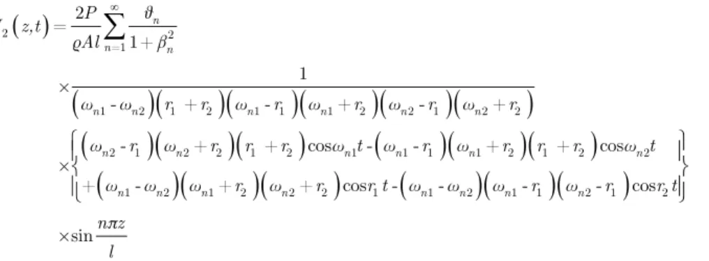
n n nn n n n n n
n n n n n n
n n n n n n n n
θ
P U z,t
ρAl
ω ω r r ω r ω r ω r ω r
ω r ω r r r ω t ω r ω r r r ω t
ω ω ω r ω r r t ω ω ω r ω r r t
nπz l
1 2
=1
1 2 1 2 1 1 1 2 2 1 2 2
2 1 2 2 1 2 1 1 1 1 2 1 2 2
1 2 1 2 2 2 1 1 2 1 1 2 1 2
2 = 1+ 1 × - + - + - +
- - + + sin + - + + sin
×
- - + + sin - - - - sin
×sin (62) 1 X 2 X 3 X
Ω
P v l O 1 X 2 XO U1
2
U
1
x ωt
t
Ω 2
x
nn n
n n n n n n
n n n n n n
n n n n n n n n
θ
P U z,t
ρAl
ω ω r r ω r ω r ω r ω r
ω r ω r r r ω t ω r ω r r r ω t
ω ω ω r ω r r t ω ω ω r ω r r t
nπz l
2 2
=1
1 2 1 2 1 1 1 2 2 1 2 2
2 1 2 2 1 2 1 1 1 1 2 1 2 2
1 2 1 2 2 2 1 1 2 1 1 2 1 2
2 =
1+
1 ×
- + - + - +
- + + cos - - + + cos
×
+ - + + cos - - - - cos
×sin
(63)
where θn is the frequency that represents the axial motion of the load, n is the Rayleigh coefficient, ωn1 and ωn2 are the positive and negative values, respectively, of the natural frequencies, and r1 and
r2 are the frequencies which describe the moving and rotating load.
To verify the VLBSE further, the deflections of the shaft are calculated here using the ANCF and are compared with the analytical solutions. The shaft is divided into four VLBSEs, with the third node placed at the point at which the load acts. The shaft section on either side of the load is divided into two elements of equal length, thereby causing the length of every element to vary as the load travels along the shaft.
To study the nature of the transient response intuitively, the deflections in the two directions are normalized with respect to Us into two non-dimensional parameters U1 /Us and U2 /Us, where Us is the static midpoint deflection of a simply supported beam of the same dimensions subjected to a static load
P at its midspan. The geometric, material, and kinematic parameters of the shaft are given in Table 4.
Parameter l 1 E ρ Ω
Value 1 m 0.02 206 GPa 7700 kg/m³ 1 rad/s
Table 4: Simulation parameters of a sppining shaft.
Two more non-dimensional parameters a and kω, which represent the load speed ratio and the number of rotations that the load completes while traversing the shaft length, respectively, are in-troduced to describe the axial speed υ and the angular speed ω of the load. Their expressions are also given by Katz (2001). In the following, the normalized deflections of the shaft are analyzed for two different sets of simulation parameters (a, kω).
(1) a=0.5, kω =1
Figure 7 shows the configurations of the shaft and its projections on the X1X3 and X2X3 planes obtained using two methods for loading point at 1/4, 2/4, 3/4, and 4/4 of the shaft length away from the origin. Figure 8 compares the ANCF and analytical solutions for the normalized deflec-tions at the loading point and the midspan of the shaft.
When the load is at 85% of the shaft length from the origin, the ANCF solution for the normal-ized deflection at the loading point in the X1 direction reaches a maximum absolute error of
−0.0085, whereas the absolute error of the ANCF normalized deflection at the loading point in the
origin, the ANCF solution for the normalized deflection at the midspan in the X1 direction reaches a maximum absolute error of −0.0049, whereas the absolute error of the ANCF normalized defl ec-tion at the midspan in the X2 direction reaches a maximum of −0.0053 at the 72% position.
(a) (b)
(c) (d)
Figure 7: Configurations of the shaft and its projections for a load at (a) 1/4, (b) 2/4, (c) 3/4, and
(d) 4/4 of the shaft length away from the origin ( =0.5,k
=
1).(a) (b)
Figure 8: Comparison of normalized deflections at (a) the loading point and (b) the midspan of the shaft ( =0.5,
1
=
k ).
0.0 0.2 0.4 0.6 0.8 1.0 -1.5
-1.2 -0.9 -0.6 -0.3 0.0 0.3 0.6 0.9 1.2
U
1
/U
s,U
2
/U
s
Z/L analytical-U1
analytical-U2
ANCF-U1
ANCF-U2
0.0 0.2 0.4 0.6 0.8 1.0 -2.4
-1.8 -1.2 -0.6 0.0 0.6 1.2
U
1
/U
s,U
2
/U
s
Z/L analytical-U1
analytical-U2
ANCF-U1
(2) a=1.5, kω =0.5
For this set of simulation parameters, the axial speed υ has been increased twofold, and the an-gular speed ω has been increased by half in comparison with the first set of simulation parameters. Figure 9 shows the configurations of the shaft and its projections on the X1X3 and X2X3 planes ob-tained using two methods for loading point at 1/4, 2/4, 3/4, and 4/4 of the shaft length away from the origin. Figure 10 compares the ANCF and analytical solutions for the normalized deflections at the loading point and the midspan of the shaft.
When the load is at 61% of the shaft length away from the origin, the absolute error of the ANCF solution for the normalized deflection at the loading point in the X1 direction reaches a max-imum of 0.0090, whereas the absolute error of the ANCF normalized deflection at the loading point in the X2 direction reaches a maximum of 0.0055 at the 84% position. When the load is at 99% of the shaft length, the ANCF solution for the normalized deflection at the midspan in the X1 direc-tion reaches a maximum absolute error of 0.0176, whereas the absolute error of the ANCF normal-ized deflection at the midspan in the X2 direction reaches a maximum of 0.0079 at the 100% posi-tion.
(a) (b)
(c) (d)
Figure 9: Configurations of the shaft and its projections for a load at (a) 1/4, (b) 2/4,
(a) (b)
Figure 10: Comparison of normalized deflections at (a) the loading point and
(b) the midspan of the shaft ( =1.5,k
=
0.5).We see from the above results that in the problem of the dynamic response of a spinning shaft subjected to an axially moving and rotating load, the numerical solutions for the normalized deflec-tions of the shaft obtained using the ANCF are in good agreement with the analytical soludeflec-tions.
This example demonstrates that in the dynamic analysis of a CCS beam with mass transporta-tion and that is spinning, the VLBSE can describe the continuum dynamics effectively.
4.4 Potential Engineering Applications of the VLBSE
Strictly speaking, a CCS beam with mass transportation at its boundaries and that is spinning is rarely used in engineering. However, in the following, we discuss several special cases in which a slender rod can be treated approximately using the proposed VLBSE.
In the drilling process of a soil-drilling sampler for planetary surface exploration (Tian et al., 2012; Deng et al., 2014; Yang et al., 2014), part of the slender drill stem is in the soil while the re-sidual is outside the soil, and the outer part is likely constrained at certain positions to avoid buck-ling. To study the dynamic behavior of the drill stem, it could be divided into several VLBSEs us-ing the constraint points and the intersection of the soil interface and drill stem as nodes to estab-lish the dynamic model.
During the turning process of a slender shaft (Lv et al., 2015; Han et al., 2012), complex inter-actions between the rotating workpiece and the translating cutter may cause excessive vibrations that not only reduce machining accuracy and lead to poor surface quality of the workpiece but also impose restrictions on production efficiency. To study the dynamic characteristics of the shaft, it could be divided into several VLBSEs using the intersection of the shaft and the cutter as one of the nodes. This dynamic model could also reflect the difference in shaft diameter on either side of the cutter due to material removal.
0.0 0.2 0.4 0.6 0.8 1.0 0.0
0.1 0.2 0.3 0.4 0.5
U
1
/U
s,U
2
/U
s
Z/L analytical-U1 analytical-U2 ANCF-U1 ANCF-U2
0.0 0.2 0.4 0.6 0.8 1.0 0.0
0.2 0.4 0.6 0.8
U
1
/U
s,U
2
/U
s
The VLBSE could also be used in the dynamic modeling of slender rods in linear motion ele-ments such as spline shafts in rotary spline screws and rotating ball splines, as well as the lead screw in a ball screw mechanism (Katz, 2001; Huang and Wang, 2014).
5 CONCLUSIONS
In this paper, we proposed a VLBSE based on the ANCF in the ALE framework. This novel ele-ment takes spinning into account, which is an effect that is neglected in most variable-length teth-er/beam elements that exist in the literature.
In addition to the position and slope vectors, the angles of rotation around the element axis of cross sections that contain two nodes are cast as generalized coordinates of the element to describe the spinning of an assumed Euler–Bernoulli beam. The material coordinates of the two nodes are also included in the ALE description to deal with mass transportation at the boundaries. Thus, there are eight coordinates in each node: the position vector, slope vector, rotational angle, and material coordinate. This novel element could therefore be used to realize the dynamic modeling of a CCS beam whose length varies because of either simple or complex transportation boundaries and for which the effect of spinning is not negligible.
Several typical numerical examples were considered based on the ANCF. These were (i) free transverse vibration analysis of an axially moving string and free flexural vibration analysis of an axially moving beam, (ii) free torsional vibration analysis of a cylindrical shaft with one end fixed and the other end free, and (iii) dynamic response analysis of a spinning shaft subjected to an axial-ly moving and rotating load. It is shown that the VLBSE could describe the dynamic behavior of a spinning CCS beam with mass transportation effectively.
Our VLBSE enriches the element library of the ANCF and allows this modeling method to be used in more types of dynamical problems in the field of flexible multi-body systems.
Acknowledgements
The authors are particularly grateful for the technical assistance from Suzhou Tongyuan Soft. & Ctrl. Tech. Co., Ltd., Associate Professor Wei Cheng and Doctor Guo Jiawen of Harbin Institute of Technology, Professor Ren Gexue of Tsinghua University, Associate Professor Tian Qiang of Bei-jing Institute of Technology.
Funding
This paper was supported by the National Defense Special Field Science and Technology Project (No. TY3Q20110005), the National Key Basic Research Program of China (Nos. 2013CB733006 and 2013CB733004) and the Self-Planned Task of State Key Laboratory of Robotics and System (Har-bin Institute of Technology) (No. SKLRS201616B).
References
Bonet, J. and Wood, R.D., (1997). Nonlinear Continuum Mechanics for Finite Element Analysis, Cambridge Univer-sity Press (Cambridge, UK).
Brenan, K.E., Campbell, S.L. and Petzold, L.R., (1996). Numerical Solution of Initial-Value Problems in Differential-Algebraic Equations, SIAM (Philadelphia).
Deng, Z.Q., Yang, S., Sun, J., Jiang, S.Y., Quan, Q.Q., Tang, J.Y., (2014). Dynamic modeling and analysis of rotat-ing mechanism in planetary soil drillrotat-ing sampler. In: 2014 IEEE International Conference on Mechatronics and Au-tomation 663-668.
Dmitrochenko, O.N. and Pogorelov, D.Y., (2003). Generalization of plate finite elements for absolute nodal coordi-nate formulation. Multibody System Dynamics 10: 17–43.
Dombrowski, S.V., (2002). Analysis of large flexible body deformation in multibody systems using absolute coordi-nates. Multibody System Dynamics 8: 409–432.
Du, J.L., Cui, C.Z., Bao, H. and Qiu, Y.Y., (2015). Dynamic analysis of cable-driven parallel manipulators using a variable length finite element. Journal of Computational and Nonlinear Dynamics 10: 011013:1–011013:7.
Dufva, K. and Shabana, A.A., (2005). Analysis of thin plate structures using the absolute nodal coordinate formula-tion. Proceedings of the Institution of Mechanical Engineers Part K-Journal of Multi-Body Dynamics 219: 345–355. García-Vallejo, D., Escalona, J.L., Mayo, J. and Domínguez, J., (2003). Describing Rigid-Flexible Multibody
Sys-tems Using Absolute Coordinates. Nonlinear Dynamics 34: 75–94.
Gatti, P.L. and Ferrari, V., (2003). Applied Structural and Mechanical Vibrations-Theory, methods and measuring instrumentation, Taylor & Francis Group (Abingdon, UK).
Gerstmayr, J. and Shabana, A.A. (2006). Analysis of thin beams and cables using the absolute nodal co-ordinate formulation. Nonlinear Dynamics 45: 109–130.
Han, X.G., Wang, M.J. and Ouyang, H.J., (2012). Establishment of vibration model and experimental analyses of workpiece with variable mass and diameter in turning process. Journal of Dalian University of Technology 52: 514– 521.
Hong, D.F. and Ren, G.X., (2011). A modeling of sliding joint on one-dimensional flexible medium. Multibody Sys-tem Dynamics 26: 91–106.
Hong, D.F., Tang, J.L. and Ren, G.X., (2011). Dynamic modeling of mass-flowing linear medium with large ampli-tude displacement and rotation. Journal of Fluids and Structures 27: 1137–1148.
Huang, L.L. and Wang, K.S., (2014). Research on reliability of dynamic performance and precision of screw drive system. Journal of Beijing Information Science and Technology University 29: 75–79.
Katz, R., (2001). The dynamic response of a rotating shaft subject to an axially moving and rotating load. Journal of Sound and Vibration 246: 757–775.
Katz, R., Lee, C.W., Ulsoy, A.G. and Scott, R.A., (1988). The dynamic response of a rotating shaft subject to a moving load. Journal of Sound and Vibration 122: 131–148.
Khan, A.A., Alam, M.N., Rahman, N.U. and Wajid, M., (2016). Finite Element Modelling for Static and Free Vibra-tion Response of FuncVibra-tionally Graded Beam. Latin American Journal of Solids and Structures 13: 690-714.
Kubler, L., Eberhard, P. and Geisler, J. (2003) Flexible multibody systems with large deformations and nonlinear structural damping using absolute nodal coordinates. Nonlinear Dynamics 34: 31–52.
Liu, Y.Z., (2012). Exact dynamical model of axially moving beam with large deformation. Chinese Journal of Theo-retical and Applied Mechanics 44: 832–838.
Lv, B.L., Li, W.Y. and Ouyang, H.J., (2015). Moving force-induced vibration of a rotating beam with elastic bound-ary conditions. International Journal of Structural Stability and Dynamics 15: 1450035:1–1450035:24.
Mikkola, A.M. and Shabana, A.A., (2003). A non-incremental finite element procedure for the analysis of large de-formation of plates and shells in mechanical system applications. Multibody System Dynamics 9: 283–309.
Omar M.A. and Shabana, A.A., (2001). A two-dimensional shear deformable beam for large rotation and defor-mation problems. Journal of Sound and Vibration 243: 565–576.
Shabana, A.A. and Yakoub, R.Y., (2001). Three dimensional absolute nodal coordinate formulation for beam ele-ments: theory. Journal of Mechanical Design 123: 606–613.
Shabana, A.A., (1996). An absolute nodal coordinates formulation for the large rotation and deformation analysis of flexible bodies, Technical Report (no. MBS96-1-UIC), University of Illinois at Chicago, USA.
Shabana, A.A., (1997). Definition of the Slopes and the Finite Element Absolute Nodal Coordinate Formulation. Multibody System Dynamics 1: 339–348.
Shabana, A.A., (2012). Computational Continuum Mechanics (2nd ed.), Cambridge University Press (New York). Sugiyama, H. and Suda,Y., (2007). A curved beam element in the analysis of flexible multi-body systems using the absolute nodal coordinates. Proceedings of the Institution of Mechanical Engineers Part K-Journal of Multi-Body Dynamics 221: 219–231.
Tang, J.L., Ren, G.X., Zhu, W.D. and Ren, H., (2011). Dynamics of variable-length tethers with application to teth-ered satellite deployment. Communications in Nonlinear Science and Numerical Simulation 16: 3411–3424.
Tian, Y., Deng, Z.Q., Tang, D.W., Jiang, S.Y. and Hou, X.Y., (2012). Structure parameters optimization and simu-lation experiment of auger in lunar soil drill-sampling device. Journal of Mechanical Engineering 48: 10–15.
Wickert, J.A. and Mote, C.D., (1990). Classical vibration analysis of axially moving continua. Journal of Applied Mechanics-Transactions of the ASME 57: 738–744.
Yakoub, R.Y. and Shabana, A.A., (2001). Three dimensional absolute nodal coordinate formulation for beam ele-ments: implementation and applications. Journal of Mechanical Design 123: 614–621.