Abstract
A 1D Finite Element model for static response and free vibration analysis of functionally graded material (FGM) beam is presented in this work. The FE model is based on efficient zig-zag theory (ZIGT) with two noded beam element having four degrees of freedom at each node. Linear interpolation is used for the axial displacement and cubic hermite interpolation is used for the deflection. Out of a large variety of FGM systems available, Al/SiC and Ni/Al2O3 metal/ceramic FGM
system has been chosen. Modified rule of mixture (MROM) is used to calculate the young’s modulus and rule of mixture (ROM) is used to calculate density and poisson’s ratio of FGM beam at any point. The MATLAB code based on 1D FE zigzag theory for FGM elastic beams is developed. A 2D FE model for the same elastic FGM beam has been developed using ABAQUS software. An 8-node biquadratic plane stress quadrilateral type element is used for modeling in ABAQUS. Three different end conditions namely simply-supported, cantilever and clamped- clamped are considered. The deflection, nor-mal stress and shear stress has been reported for various models used. Eigen Value problem using subspace iteration method is solved to obtain un-damped natural frequencies and the corresponding mode shapes. The results predicted by the 1D FE model have been com-pared with the 2D FE results and the results present in open litera-ture. This proves the correctness of the model. Finally, mode shapes have also been plotted for various FGM systems.
Keywords
Finite Element, MROM, ZIG-ZAG Theory, Functionally Graded Beam, Abaqus.
Finite Element Modelling for Static and Free
Vibration Response of Functionally Graded Beam
1 INTRODUCTION
In case of composite materials where two distinct materials (e.g. metal and ceramic) with significant difference in material properties are bonded together, large jump in the in-plane normal stresses and
Ateeb Ahmad Khan a
M. Naushad Alam b
Najeeb ur Rahman c
Mustafa Wajid d
a, b, c, d Department of Mechanical
Engi-neering, ZHCET, Aligarh Muslim Univer-sity, Aligarh.
a [email protected] b [email protected] c [email protected] d [email protected]
http://dx.doi.org/10.1590/1679-78252159
high-transverse shear stresses occur at the interface during fabrication and operation. This leads to delamination at the interface and poor load-bearing performance. Developments in materials engi-neering lead to a new type of composites with smoothly and continuously varying thermos-mechanical properties that are called functionally graded materials (FGMs). Functionally graded materials (FGMs) provide an elegant solution to this problem, wherein the abrupt change in composition of material from one layer to another is replaced by layers of gradually varying microstructure and composition. FGM structures have various advantages over the composite laminates, such as smaller stress concentrations, smaller thermal residual stresses and the possibility to achieve specific for different applications. This concept has found many potential applications like thermal and cor-rosion barriers, medical implants, lightweight armour material with high-ballistic efficiency, etc. FGMs are made by combining different materials through complex processes such as powder metal-lurgy methods, physical and chemical vapor deposition, solid freeform fabrication etc. Detailed process for manufacturing FGM’s and various areas of application are presented by Rasheedat M. et al.
Among the various models which have been proposed to predict the effective elastic properties of two-phase materials, the self-consistent model of Hill (1965), the Mori and Tanaka (1973), the linear rule of mixtures and in Jones (1999) the intermediate rule of mixtures provide simple and convenient ways for predicting the overall response. For kinematic modelling, several one-dimensional (1D) beam and 2D plate theories such as Cho and Oden (2000) applied CLT (Classical Laminate Theory) for thermal stress analysis of infinite functionally graded beams and plates with layer-wise compositional change, Nguyen et al. (2008) found the effect of transverse shear stresses by energy equivalence using FGM models based on FSDT theory. The transverse shear stresses are obtained using the membrane stresses and various equilibrium equations and Sina et al. (2009) developed a new beam theory dif-ferent from the traditional first-order shear deformation beam theory is used to analyze free vibration of functionally graded beams. The beam properties is varied through the thickness according to simple power law distribution in terms of volume fraction of material constituents. It is assumed that the lateral normal stress is zero and the governing equations of motion are derived using Hamilton’s principle. Reddy (1983) developed a higher order shear deformation theory of composites. This theory accounts for the parabolic distribution of the transverse strains through the thickness of the structure. This theory has been found to be predicting deflection and stresses more accurately than FSDT. Cheng and Batra (2000) exploited Reddy’s third-order plate theory to study buckling and steady state vibrations of a simply supported functionally gradient isotropic polygonal plate resting on a Winkler Pasternak elastic foundation and subjected to uniform in-plane hydrostatic loads. Sankar (2001) presented an elasticity solution for simply supported FG beams subjected to sinusoidal trans-verse loading. Kapuria et al. (2008) have presented an efficient zigzag model and its experimental validation for thermo-elastic static and free vibration response of Al/SiC and Ni/Al2O3 FGM beams.
Results indicate that position of neutral surface is very important in functionally graded materials. Kadoli et al. (2008) implemented displacement field based on higher order shear deformation theory to study the static behavior of functionally graded metal–ceramic (FGM) beams under ambient temperature. FGM beams with variation of volume fraction of metal or ceramic based on power law exponent are considered. Najeeb and Alam (2012) presented a one dimensional finite element model using an efficient layerwise (zigzag) theory for the dynamic analysis of laminated beams integrated with piezoelectric sensors and actuators. Mohanty et al. (2012) presented the evaluation of static and dynamic behavior of functionally graded ordinary (FGO) beam and functionally graded sandwich (FGSW) beam for pined–pined end condition. The variation of material properties along the thickness is assumed to follow exponential and power law. A finite element method is used assuming first order shear deformation theory for the analysis. Furqan and Naushad (2013) assessed higher order theory of laminated beams under static mechanical loads. The Third order theory and First order shear deformation theory are assessed by comparison with the exact two-dimensional elasticity solution of the simply-supported beam. Mehta et al. (2013) used finite element method in modelling the dynamic behavior of FGM to determine its natural frequency. The properties in the functionally graded ma-terial are assumed to vary according to power law. The natural frequencies were obtained for FG beams under various boundary conditions including Clamped-Fixed, Simply supported-Fixed, Clamped-Clamped, Simply supported-Simply-supported, and Clamped-Simply supported. Shi-rong Li et al. (2014) studied the free vibration of functionally graded material (FGM) beams based on both the classical and the first-order shear deformation beam theories. Nguyen et al. (2014) presented the analytical solutions for the static analysis of the transversely or axially functionally graded beams with tapered cross-section. The elastic modulus of the beam varies according to the power form.
The present study deals in developing a 1D FE model based on Zigzag theory for FGM elastic beams using MATLAB as a mathematical tool. The model is used to compute the deflection, stress and shear stress at various values of side to thickness ratio and upto first five fundamental frequency. A 2D FE model for the same elastic FGM beam has been developed using ABAQUS software. The results predicted by the 1D FE model have been compared with the results obtained using 2D FE model. These predicted results have also been compared with the results presented in the open liter-ature. This is done to prove the correctness of the FE model developed. A three layer Al/SiC beam, five layer Ni/Al2O3 and ten layer Ni/Al2O3 beam is modelled for the analysis purpose. Mode shapes
has also been plotted for these FGM system under various boundary conditions viz. simply supported, clamped-clamped and cantilever.
2 MATERIAL MODELLING
For the bi-material FGM systems, the volume fractions Vc and Vm of the ceramic and the metal as
taken by Kapuria et. al (2006) are assumed to vary along z-direction according to following power law:
.5 / ,
.5 ,
(z) = 1– (z)
Figure 1:Variation of volume fraction of metal across the non-dimensional thickness.
Where M is a non-negative real number called the inhomogeneity parameter. The variation of Vm
across z is plotted for M = 4. The volume fraction for a layer is computed at the center of the respective layer.
The effective material properties for a layer are computed using different averaging methods based on volume fraction at the centre of layer. The effective material elastic modulus E of a layer is computed using the modified rule of mixtures (MROM), which was originally proposed for cemented carbides by Tomota et al (1976) and later adopted for FGM by many researchers Cho and Oden (2000).
According to this approach, the two phase material is treated as an isotropic composite for which uniaxial stress σ, strain ɛ, are related to constituent stresses , andɛ , ɛ as,
σ = Vm + Vc,
ɛ = ɛ Vm + ɛ Vc, (2)
and
q = [( – )/ (ɛ – ɛ )] (3)
Where q is Stress to Strain transfer ratio between two phases.
The value of q for Al/SiC has been experimentally determined by Kapuria et. al (2008) to be 91.6 GPa, which is used in this work for computing the elastic modulus of Al/SiC FGM samples. For Ni/Al2O3 system, the value of q is taken as 4.5 GPa as used by Kapuria et. al (2008).
Now the Young’s modulus E of the FGM material can be calculated explicitly using MROM as,
E = [ (q+ )/(q+ )+(1– ) ]/[ (q+ )/(q+ )+(1– )] (4)
For this work, other material property i.e. Poisson’s ratio and density ⍴ have been calculated using linear rule of mixture (ROM) as:
= Vm + Vc
3 TYPES OF BEAM
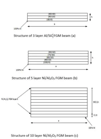
Figure 2:Geometry and Volume fraction variation through thickness for the FGM beams.
Three Functionally graded beams are considered in this paper, namely beam (a), beam (b) and beam (c). All three beams are combination of metal and ceramic with bottom of the beam being metal rich and top of the beam being ceramic rich. Beam (a) is a three layered fgm beam of Al/SiC and the volume fraction each layer is pre-defined as shown in figure 2. Beam (b) is a 5 layered fgm beam of Ni/Al2O3 and in this beam also the pre-defined volume fraction is shown in the figure 2.
Beam (c) is a 10 layered fgm beam of Ni/Al2O3 and is bit different from the other two beams. In
beam (c) each layer is of equal thickness i.e. 0.1h and the bottom most layer is of pure metal. Moreover, the volume fraction of the remaining nine layers is computed using equation 1. Young’s modulus and Density of each layer is calculated using MROM and ROM respectively.
4 ZIG-ZAG THEORY FOR FGM BEAM
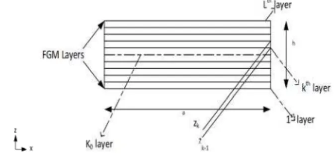
gradient of volume fractions of the constituents. The axes along the length, width, and thickness are x, y, z, respectively. The loads given to the beam do not vary along thickness direction.
Figure 3:Geometric Description of Layered Elastic FGM Beam.
The mid plane of the beams is chosen as the xy-plane with
z = = – (h/2)
and
z = =(h/2)
being the bottom and top surfaces.
The z-co-ordinates of the bottom surface of the k-th layer (numbered from bottom) is denoted as . The reference plane z=0 either passes through or is the bottom surface of the layer. For beam of small width, assumptions for mathematical simplifications of 1-D model are-
(i) State of plane stress ( = = =0)
(ii) Transverse normal stress neglected ( =0)
(iii) Axial and transverse displacement considered independent of y.
For ZIGT, w is approximated by integrating the constitutive equations for ɛ by neglecting the contribution of . Thus, constitutive equation for ɛ is
ɛ = , = (6)
According to the basic assumption of the zigzag theory,
w (x , z , t ) = (x , t) (7)
For ZIGT the axial displacement u is assumed as a combination of a third order variation across the laminate thickness with a layerwise linear variation. So, for layer,
u(x,z,t) = (x,t) - z (x,t) + z (x,t) + z2 (x,t) + z3η(x,t) (8)
= , + , ,= , + +2z +3 η + , = + 2z +3 η (9)
= = ( +2z + 3z2η) (10)
u (x,z,t) = (x,t) – z , ( x,t) + (z) (x,t) (11)
4.1 Equation of Motion
The Hamilton’s principle is represented as below,
⍴ – ɛ )dV + )dƬ=0 (12)
Let , be the normal forces per unit area on the bottom and top surfaces of the beam in direction z. The extended Hamilton’s principle for the elastic beam can be expressed as, using notation
... =
1
1
k
k
z L k
z
bdz
And integrating the term
ku
iu
i by parts for now a beam of length a under above mentioned loading condition. The principle equation given by Eq. (12) reduces to the form0
[
a k
u
u +
kw
w + x x + zx z x > –b 1 zp w(x,
z
0 , t) + bp2z w(x ,z
L , t)]–< x u zx w >|a =0
(13)
∀ u0 , w0 , 0. This variational equation is expressed in terms of u0 , w0 , 0 to yield
equations of motions and boundary conditions.
In the above equation, u and w can be expressed as
u = f1(z)u1
u = f1(z)u1 = 1 1 T T
u f (z) (14)
with
1
u =
0
0,
0
x
u w
1
f (z) =
1
k z
R z
(15)
<
ku
u + kw w > = <1 1
T T
u f (z) f1(z)u1 + w0w0>= 1 T
u Iu1 + w I0 22w0 (16)
where inertia I and I22 are defined as
I =
11 12 13
12 22 23
13 23 33
I I I
I I I
I I I
= < 1 T f
(z) f1(z)> =
T
I (17)
with elements explicitly given as,
[I11 , I12 , I13 ] = <
k
[1, z, kR (z)] >
[I22 , I23 ] = <
k
z [z, kR (z)] >
[I33 ] = <
k
kR (z) [Rk(z)] >
(18)
The strain increments x and zx are related to virtual displacements by,
x
= u,x + w0 ,x w0 ,x
= f1(z) 1 + w0 ,x w0 ,x
(19)
zx
= u,x + w0 ,x
= , k z
R
0 (20)with 1 = 0, 0, 0, x xx x u w (21)
The strain energy term in variational equation Eq. (13) expressed as
x
x + zx zx> = <[ 1 1 T T
f
(z)+ w0 ,x w0 ,x]x + 0 , kz zx
R
>= 1 1
T F
+ 0 Qx + w0 ,xN wx 0 ,x(22)
Where beam stress resultants are defined as
1
F =
x x x N M P (23)
[Nx , Mx , Px , Qx ] = < [1, z , k
R (z) , , k
z
R
(z) ] > (24)2
F = b ( 1 z
p + p2z ) (25)
At last, the terms due to load at the end of the beam are expressed as,
x
u + zx w > =– < 1 1 T T
u f (z)x+zx w0>
= – [ u F1T 1 + Vx w0]
= – [ * * * *
0 0
x x
N u V w -
M
*x
w
0,*x + Px*0* ](26)
Where the superscript * represents the mean value at the ends and Vx = < zx> Substituting all above calculated sub-parts in the original equation Eq. (13), we have
0
[
a
1 Tu Iu1 + w I0 22w0 + u0 ,xNx – w,x xM x + Px0 ,x + 0 Qx + w0 ,xN wx 0 ,x
– F2w0]
dx
– [* * * *
0 0
x x
N u V w –
M
x*
w
0,*x + Px*0* ] = 0(27)
5 FINITE ELEMENT MODEL FOR FGM BEAM
A two noded element, having four degrees of freedom at each node, finite element model is developed for the analysis of elastic layered FGM beams under various kinds of mechanical loading employing 1-D zigzag theory presented earlier.
The stress resultants Nx, Mx, Px , Qx in eq. (24) can be related to u0, w0, 0 as:
x x x x N M P Q = 0,
11 12 13
0,
12 22 23
0,
13 23 33
0 22
0 0
0 0 0 0
x
x
x
u
A A A
w
A A A
A A A
A (28)
where, if A represents the beam stiffness matrix, and is given by,
A =
11 12 13
12 22 23
13 23 33
A A A
A A A
A A A
= T
A (29)
Now, the beam stress resultants from Eq. (23) can be expressed as below,
1
F = A1
with
x
Q = A2 20 (30)
The elements of above matrices are:
[A11 , A12 , A13 ] = < 11
ˆ
Q
[ 1 , z , kR (z) ] >,
[A22 , A23 ] = < 11
ˆ
Q
z [ z kR (z) ]>,
[A33 ] = < 11
ˆ
Q
kR (z) [ Rk(z) ] >,
[A22 ] = <
Q
ˆ
55 , kz
R
[ , kz
R
(z) ] >,We can define stresses , strains , and stress resultant in a condensed form and call them as generalised stress ,generalised strain and generalised stress resultant respectively as,
ˆ
u u0 w0,x 0 w0 T; ˆ
= [u0 ,x w0 ,xx 0 ,x 0 ]T;
F = [Nx Mx Px Qx ]T;
(32)
also,
ˆ
F = Dˆ ,
and D = 22
0
0
A
A
(in condensed form) (33)5.1 Interpolation Function for FG Beam Element
As described above, a two noded element, having four degrees of freedom at each node, has been used for interpolating the mechanical variables for zigzag theory. Since the highest derivative of u0 ,w0 ,
0
in the variational equation are u0,x ,w0,xx , 0 ,x , therefore to meet the convergence requirement of finite element method , u0 and 0 must be C
0 continuous and 0
w should be C1-continuous at the
element boundaries. Thus, u0 and 0 have been interpolated using Lagrange interpolation function
and w0 has been interpolated using Hermite cubic interpolation function. Also, it is evident that as
zx
is dependent on 0 only and not on w0 ,x , this interpolation scheme will not lead to shear locking. Denoting the values of an entity (.) at node i by (.)i, u0,w0, 0 are interpolated in an element
of length a as
0
u = N 0 e
u , 0 = N 0 e
, w0 = 0
e
N w (34)
Where the elemental variable matrices 0 e u , 0
e w , 0
e
are given by
0 e
u =
1 2
0 0
T
u u
, 0
e
= 0 1 02
T
, 0
e
w = 01 0,1 02 0,2
T
x x
w w w w
(35)
The interpolation function N and N are given by
N = [N N1 2 ]
2 3 4
1
where,
1
N =1- (x/a)
2
N = (x/a)
1
N
1
3 2/ 2
2 3/ 3
x a x a
2
N
x
(2
x
2/ ) (
a
x
3/
a
3)
2 2
3 3 3
N
3
x
/
a
2x / a
2 4
N
x
/
a
3 2/ x a
(36)
Now if we define the generalized displacement vector at element level as
T T T T
e e e e
U u w (37)
The generalized displacement vector uˆ and generalized strain vector ˆ can be expressed in terms
of e
U as:
ˆ
u =NUˆ e ,
ˆ B Uˆ e
, (38)
where,
ˆ
N = ,
0 0 0 0 0 0 0 0 x N N N N ˆ B =
, , , 0 0 0 0 0 0 0 0 x xx x N N N N
(in compressed form)
(39)
5.2 Element Inertia Stiffness and Load Vector
The contribution Te of one element of length a to the integral is expressed as
e
T =
0
ˆ ˆ [ ˆ
a T
u I u
+
ˆ
TD
ˆ
u f
ˆ
T u]dx
(40)ˆ I =
22 0 0 I I , u
f =
0 0 0 2
T F(41)
If we substitute the expressions for uˆ and ˆ from Eq. (38) in the expression for e
T we get,
e
T =
0
[ ˆ ˆ ˆ ˆ ˆ ˆ ˆ ]
T
a
e T e T e T
u
U N IN U B DBU N f dx
= UeM Ue eK Ue ePe
(42) where, 0
ˆ ˆ ˆ
a
e T
M
N INdx ,a
e T
0
K
B D dxˆ ˆ ˆB ,0
ˆ
a
e T
u
P
N f dx(43)
The distributed pressure loads 1 z p , 2
z
p are linearly interpolated in terms of their nodal values given by 1e
z
p and p2ze, respectively, as
1 z
p = Np1ze , 2
z
p =Np2ze, (44)
with
1e z p =
1 2 1 1 z z p p , 2 z p =
1 2 2 2 z z p p ,
On substituting the expressions for Nˆ and
u
f in the integral for Pe, it yields,
0
ˆ
a
e T
u
P
N f dx = 20
0
0
a T
N F dx
2
F = bN ( 1e z
p + p2ze), Until here the elemental degrees of freedom were arranged as
e
U =
1 2 2 1 2
01 02 01 0, 0 0, 0 0
T
x x
u u w w w w
(46)
However, for convenience, these elemental degrees of freedom have been arranged like below,
e
U =
1 1 2 2 2
01 01 0, 0 02 0 0, 0
T
x x
u w w
u w w
(47)
Accordingly the elemental matrices have also been rearranged by changing the indices from [1,2,3,4,5,6,7,8] to [1,5,2,3,6,7,4,8] respectively.
5.3 System Equations and Boundary Conditions
Summation of all the elements of e
T to the variational integral, the system equation is obtained
as
MU + KU = P, (48)
In which the M, K, P matrices are assembled from their elemental matrices respectively. In case of point loads applied at nodes are added to P, at locations corresponding to their degrees of freedom numbers.
The variationally consistent boundary conditions at the beam ends are obtained as,
0
u = u0 or Nx = Nx,
0
w = w0 or Vx = Vx,
0 ,x
w = w0 ,x or Mx = Mx,
0
= 0 or Px = Px,
(49)
The geometric boundary conditions for various end conditions are as follows, Simply supported:
x
N = 0, (movable) u0 = 0 (immovable)
0
w = 0, Mx = 0, Px = 0
Clamped:
0
u = 0, 0 = 0,
0
w = 0, w0 ,x = 0
Free:
x
N = Nx Px = Px
x
6 ABAQUS MODELLING
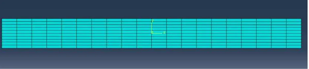
The structure of various beams that are used are shown in Figure 2. The thickness of the beam is taken as unity and the length of the beam is taken corresponding to side-to thickness ratio. The global x-coordinate is taken along the length of the beam and the global y-coordinate is taken along the thickness. The model is developed using 20 elements along the axial direction and 1 elements in each layer along the thickness direction. Three different boundary conditions are taken into account viz. simply-supported, cantilever and clamped- clamped. The beam is analyzed for deflections and stresses under various boundary condition when the beam is subjected to load working along the Y- direction for various side-to-thickness ratios (a/h). The figure below shows the meshed model of beam (c). The center deflection and stresses are presented here in non-dimensional form.
Figure 4:Meshing of 10 layer Ni/Al2O3 beam (c) FGM beam.
7 RESULTS AND DISCUSSION
The validation of zigzag theory FE model developed is presented for static and free vibration response of FGM beams. The material properties and stress to strain transfer ratio for Al /SiC and Ni /Al2O3
systems is taken up from Kapuria et al. (2008). This ratio is used to predict effective elastic modulus of both the FGM systems using MROM. The static analysis and free vibration response of layered FGM beams, with ceramic content varying from 0 to 40%, has been presented here. The material properties of the basic constituents Al, SiC, Ni and Al2O3 of the FGM beams, considered for
compu-ting the effective properties of the layers, as used by Kapuria et. al (2008) are listed in Table 1. The young’s modulus of the different layers of the beam are computed using MROM while density of the different layers of the beam are computed using ROM.
Property Unit Ni Al2O3 Al SiC
E GPa 199.5 393.0 67.0 302.0
- 0.3 0.25 0.33 0.17
⍴ Kg /m3 8900 3960 2700 3200
Table 1:Constituent Properties of materials used.
The following mechanical load cases are considered:
1.Uniformly distributed load at the top surface of the beam (load case 1)
2 z
p = p0,
2.Sinusoidally varying load over the top surface of the beam (load case 2)
2 z
p = p0sin (πx/a),
where x gives the location of any point on the beam and ‘a’ is the total span of the beam. The p0is a
constant with magnitude 1.
The results that are presented have been non-dimensionalised using following expressions
w
= (100*w*Y
0)/hS4p0 ,
x = (x/S2 0
p ), zx = (100zx)/Sp0,
with,
S = a/h, Y0 = 127.8295 GPa (For Ni/Al2O3) = 88.509 GPa (For Al/SiC)
The dimensionless entities are chosen such that their values are almost independent of S for different beams.
7.1 Static Response
The 2D FE results for
w
, x, and zx at points across the thickness are given in Table 2 and Table 3 for elastic beam (c) and for inhomogeneity parameter M = 4. Table 2 shows the result for load case 2 for span to thickness ratio S = 5, 10 and 40. The load is applied at the top surface of the beam. The non-dimensionalized deflection,w
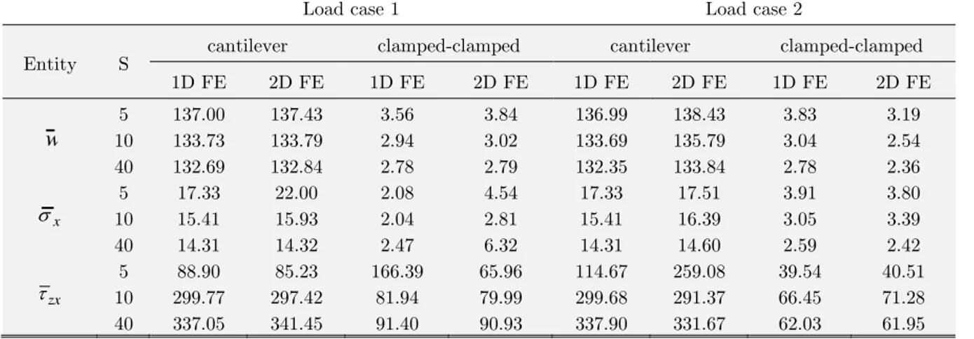
is reported at the top surface. The observed error for simply supported beam (c) with load case 2 on comparison with Kapuria et al. (2006) is within 3% for thick beam with S = 5. For moderately thick beam, S = 10 error is within 7%.The 1D FE based on zig-zag theory and 2D FE Abaqus results are presented in Table 3 for beam (c) with cantilever and clamped-clamped end conditions for aspect ratios S = 5, 10 and 40 and inhomogeneity parameter M = 4. Table shows the results in bending for both the load cases i.e. sinusoidally varying and uniformly distributed load. Further, it can be seen from the table that the results are in close agreement with each other, which eventually shows the correctness of the FE model presented.
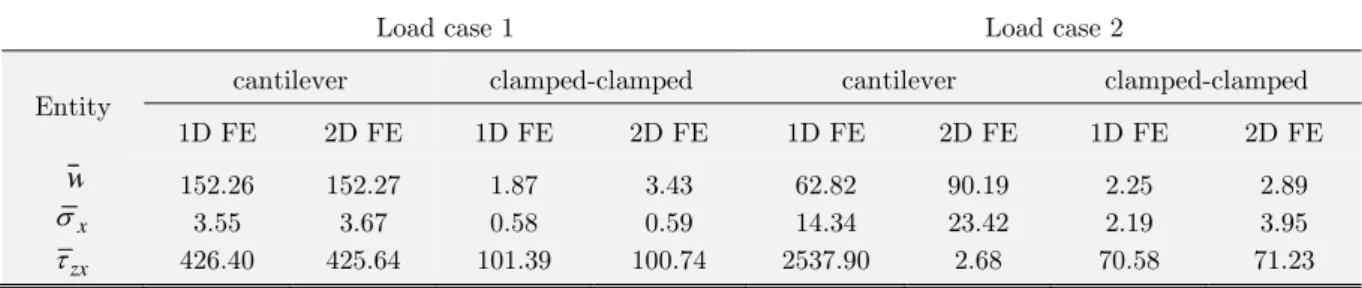
The Tables 4 and Table 5 present the results for 3 layered beam (a) with Al/SiC FGM system under sinusoidally varying load and uniformly distributed load for different boundary conditions. The inhomogeneity constant for each case is M = 4.
A different FGM system is considered in Tables 6 and Table 7. The results are presented for 5 layered Ni / Al2O3 FGM beam (b) under sinusoidally varying load and uniformly distributed load on
Finally, it can be observed that the results obtained using 1D FE model are in good agreement with the results obtained using 2-D FE abaqus, which proves the correctness of the 1-D zig-zag theory based FE model.
Load case 2
Entity S Kapuria et al. (2006) 2D FE
w 5 10 40 -11.3 -10.55 -10.31 -11.60 -11.08 -10.94
10x
5 10 40 7.82 7.73 7.69 7.49 7.45 7.44 zx
105 40 -45.92 - 46.02 -46.04 -46.53 -45.83 -46.69
Table 2:Static response of 10 layer FGM beam (c) for simply supported end condition with M=4.
Load case 1 Load case 2
Entity S cantilever clamped-clamped cantilever clamped-clamped
1D FE 2D FE 1D FE 2D FE 1D FE 2D FE 1D FE 2D FE
w 5 10 40 137.00 133.73 132.69 137.43 133.79 132.84 3.56 2.94 2.78 3.84 3.02 2.79 136.99 133.69 132.35 138.43 135.79 133.84 3.83 3.04 2.78 3.19 2.54 2.36 x
10 5
40 17.33 15.41 14.31 22.00 15.93 14.32 2.08 2.04 2.47 4.54 2.81 6.32 17.33 15.41 14.31 17.51 16.39 14.60 3.91 3.05 2.59 3.80 3.39 2.42 zx
10 5
40 88.90 299.77 337.05 85.23 297.42 341.45 166.39 81.94 91.40 65.96 79.99 90.93 114.67 299.68 337.90 259.08 291.37 331.67 39.54 66.45 62.03 40.51 71.28 61.95
Table 3:Static response of 10 layer Ni/Al2O3 FGM beam (c) with M=4.
Load case 1 Load case 2
Entity 1D FE 2D FE 1D FE 2D FE
w x zx 16.11 6.20 75.64 16.05 6.64 77.33 82.55 20.42 267.95 90.19 23.42 268.28
Load case 1 Load case 2
Entity cantilever clamped-clamped cantilever clamped-clamped
1D FE 2D FE 1D FE 2D FE 1D FE 2D FE 1D FE 2D FE
w x zx 152.26 3.55 426.40 152.27 3.67 425.64 1.87 0.58 101.39 3.43 0.59 100.74 62.82 14.34 2537.90 90.19 23.42 2.68 2.25 2.19 70.58 2.89 3.95 71.23
Table 5:Static response of 3 layer Al/SiC FGM beam (a) with M=4.
Load case 1 Load case 2
Entity 1D FE 2D FE 1D FE 2D FE
w x zx -14.36 -8.76 - 74.83 - 14.29 -8.05 -73.03 -9.21 -4.09 -48.18 -11.27 -5.53 -47.22
Table 6:Static response of FGM beam (b) for simply supported end condition with M=4.
Load case 1 Load case 2
Entity cantilever clamped-clamped cantilever clamped-clamped
1D FE 2D FE 1D FE 2D FE 1D FE 2D FE 1D FE 2D FE
w x zx -135.91 3.42 445.52 -135.7 3.47 431.67 -3.06 -5.18 -78.85 -3.12 -6.17 -73.44 -82.65 -26.54 -327.70 - 80.40 -22.09 -321.32 -2.75 4.66 50.87 -2.94 4.68 51.46
Table 7:Static response of 5 layer Ni/Al2O3 FGM beam (b) with M=4.
7.2 Free Vibration Response
The convergent FE results for natural frequencies are obtained by modelling the FGM beams for both of the considered FGM systems viz. Al/SiC and Ni/Al2O3 and for different boundary conditions. The
predicted natural frequencies, n of first few modes (using MROM and linear ROM based property estimates) obtained from 1D FE zigzag model are compared with 2D FE results. All the frequency values are given with unit Hz. An 8-node biquadratic plane stress quadrilateral type element, CPS8R is used for modeling in ABAQUS. Along the beam length 80 elements and 15 elements were seeded along thickness direction. The results for natural frequencies are validated with results presented in Kapuria et al. (2008). These results are presented in Tables 8 to Table 9. It can be seen that present beam model in conjunction with MROM with the value of q as 91.6 GPa (Kapuria et al. (2008)) predicts fundamental natural frequencies of 3 layer Al/SiC cantilever beams very accurately with maximum error of 1.35% and for clamped-clamped boundary condition with maximum error of 5.60%.
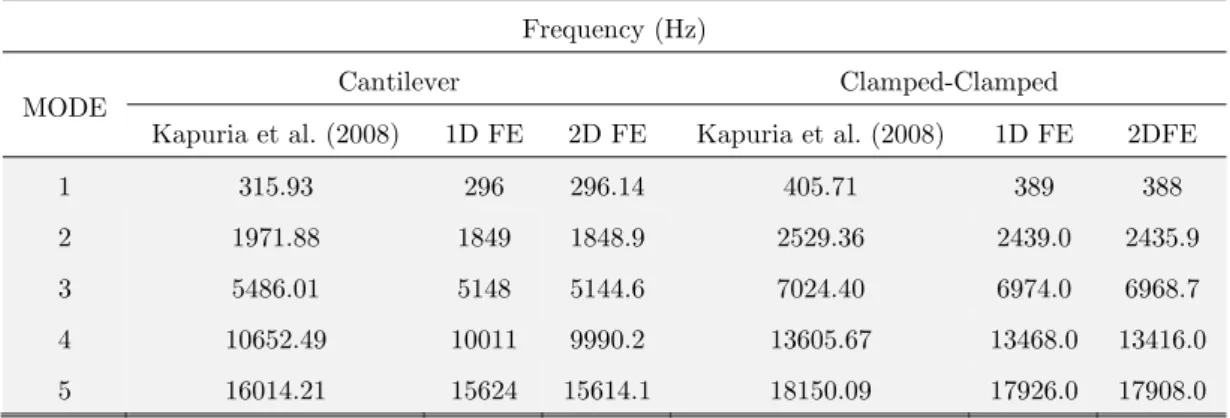
In case of 5 layer Ni/Al2O3 FGM system, beam (b) has been modelled using 1D FE as well as 2D
to have maximum error of 2.86% in case of cantilever and 12.9% maximum error in case of beam clamped at both the ends. Here the q value is taken to be 4.5 GPa (Kapuria et al. (2008)). Close agreement of the theoretical model results with the results presented in Kapuria et al. (2008) proves consistency and robustness of 1D FE model and thus using it, the fundamental frequencies of the two foresaid FGM systems for simply supported boundary conditions are presented in Table 11. From Table 11 it can be seen that the natural frequencies obtained using 1D FE model are in good agree-ment with 2D FE results for all three different beams. Also, a 10 layer Ni/Al2O3 beam model has
been considered for frequency analysis. The results for 10 layer Ni/Al2O3 beam are presented in Table
10. All the 1D FE results are in good agreement with 2D FE results obtained using ABAQUS.
Frequency (Hz)
MODE Cantilever Clamped-Clamped
Kapuria et al. (2008) 1D FE 2D FE Kapuria et al. (2008) 1D FE 2DFE
1 811.46 809 810.09 1035.48 1006.78 1004.28
2 4913.67 4902 4899.1 6206.14 6040 6019.2
3 13096.07 13087 13035.0 16052.86 15840 15662
4 14449.23 14254 14258 16365.32 16196.58 16028.93
Table 8:Natural Frequencies of 3 layer Al / SiC FGM beam under various end conditions for M =4.
Frequency (Hz)
MODE Cantilever Clamped-Clamped
Kapuria et al. (2008) 1D FE 2D FE Kapuria et al. (2008) 1D FE 2DFE
1 315.93 296 296.14 405.71 389 388
2 1971.88 1849 1848.9 2529.36 2439.0 2435.9
3 5486.01 5148 5144.6 7024.40 6974.0 6968.7
4 10652.49 10011 9990.2 13605.67 13468.0 13416.0
5 16014.21 15624 15614.1 18150.09 17926.0 17908.0
Table 9:Natural Frequencies of 5 layer Ni / Al2O3 FGM beam under various end condition for M = 4.
Frequency (Hz)
MODE Cantilever Clamped-Clamped
1D FE 2D FE 1D FE 2DFE
1 6.87 7.67 19.08 19.11
2 41.42 42.09 73.52 73.53
3 109.99 109.66 156.56 156.32
4 116.36 232.38 232.22 232.38
5 201.76 303.37 260.61 256.76
Frequency (Hz)
MODE Beam (a) Beam (b) Beam (c)
1D FE 2DFE 1D FE 2DFE 1D FE 2DFE
1 2255.0 2255.8 831 830.71 5.56 6.87
2 8692.0 8701.3 3309 3308.9 33.89 41.42
3 18529.0 18558.0 7396 7394.2 91.11 99.76
4 28574.0 28441.0 13038 13024 104.69 116.36
Table 11:Natural Frequencies of simply supported FGM beams for M = 4.
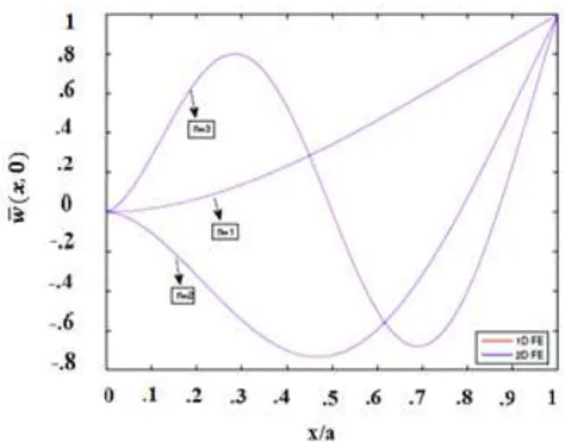
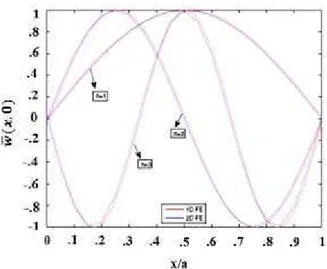
The mode shapes for mid-surface deflection for the first three flexural modes (n = 1, 2, 3) have been plotted using 2D FE model. The 2D FE mode shapes have been plotted using the values that are normal-ized with the maximum deflection values. They have also been obtained by using zigzag 1D FE analysis and are compared with the 2D FE results. They have been presented in Fig 5 to Fig 13 for moderately thick beam (S = 10), respectively for different boundary conditions. This comparison shows their close agreement with each other. Therefore they can be trustfully used for future references.
Figure 5:First three flexural mode shapes of 3 layer Al/SiC FGM beam for cantilever end condition.
Figure 7:First three flexural mode shapes of 3 layered Al/SiC FGM beam for clamped-clamped end condition.
Figure 8:First three flexural mode shapes of 5 layer Ni/Al2O3 FGM beam for cantilever end condition.
Figure 10:First three flexural mode shapes of 5 layer Ni/Al2O3 FGM beam for simply-supported end condition.
Figure 11:First three flexural mode shapes of 10 layer Ni/Al2O3 FGM beam for cantilever end condition.
Figure 13:First three flexural mode shapes of 10 layer Ni/Al2O3 FGM beam for clamped-clamped end condition.
Table 12 shows sensitivity analysis i.e. the effect of dividing the FG beams into different number of layers on natural frequencies using the developed 1-D FE model. Non-dimensional natural frequen-cies up to third mode of vibration are computed for span-to-thickness ratios 5 and 20. The beam used by Thai and Vo (2012) is divided into 8-layers, 10-layers and 12-layers of equal thickness and the results are compared with Thai and Vo (2012). The material properties and boundary conditions are taken from Thai and Vo (2012). Young’s modulus and density for each layer are calculated using the linear rule of mixture at the center of each layer. Poisson’s ratio is assumed to be constant. The inhomogeneity parameter (M) is taken as 5.
S MODE 8-layer 10-layer 12-layer Thai and Vo (2012)
5
1 2.521 2.780 3.166 3.401
2 10.562 10.750 11.052 11.543
3 19.829 20.385 21.237 21.716
20
1 2.684 3.075 3.438 3.836
2 14.183 14.421 14.726 15.162
3 31.514 32.064 32.894 33.469
Table 12:Non-dimensional natural frequencies of simply supported FGM beams for M = 5.
Figure 14:Sensitivity analysis of frequency in terms of number of layers for span to thickness ratio, S=5 of FG beam.
Figure 15:Sensitivity analysis of frequency in terms of number of layers for span to thickness ratio, S=20 of FG beam.
8 CONCLUSIONS
layers of FG beam shows that the computed results approach to the exact result as the number of layers are increased. FGM beam can also be modelled as layer wise using the developed 1D FE model.
References
ABAQUS/Standard User's Manual, Version 6.10, Vol. 1 (2010).
Alshorbagy, A.E., Eltaher, M.A., Mahmoud, F.F., (2011). Free vibration characteristics of a functionally graded beam by finite element method, Applied Mathematical Modelling, 35:412–425.
Cheng, Z.Q., Batra, R.C., (2000). Exact correspondence between eigenvalues of membranes and functionally graded simply supported polygonal plates, J. Sound and Vibration. 229:879–895.
Cho, J.R., Tinsley, O.J., (2000). Functionally graded material: a parametric study on thermal-stress characteristics using the Crank-Nicolson-Galerkin scheme, Computer Methods in Applied Mechanics and Engineering, 188:17-38. Furqan, M., Alam, M.N., (2013). Modelling and Analysis of Laminated Composite Beams using Higher Order Theory, AMAE, Int. J. on Manufacturing and Material Science, 3:8-13.
Hadi, A., Daneshmehr, A.R., Mehrian, S.M.N., Hosseini, M. and Ehsani, F., (2013). Elastic Analysis of Functionally Graded Timoshenko Beam Subjected To Transverse Loading, Technical Journal of Engineering and Applied Sciences, 3:1246-1254.
Hill, R., (1965). A self-consistent mechanics of composite material, Journal of Mechanics and Physics of Solids, 13:213– 222.
Jones, R.M., (1999). Mechanics of Composite Material, Second Edition.
Kadoli, R., Akhtar, K., Ganesan, N., (2008). Static analysis of functionally graded beams using higher order shear deformation theory, Applied Mathematical Modelling, 32:2509-2525.
Kapuria, S., Bhattacharyya, M., Kumar, A.N., (2006). Assessment of coupled 1D models for hybrid piezoelectric layered functionally graded beams, Composite structures, 72:455-468.
Kapuria, S., Bhattacharyya, M., Kumar, A.N., (2008). Bending and free vibration response of layered functionally graded beams: A theoretical model and its experimental validation, Composite Structures 82:390–402.
Li, S., Wan, Z., Zhang, J., (2014). Free vibration of functionally graded beams based on both classical and first-order shear deformation beam theories, Applied Mathematics and Mechanics, 35:591-606.
Mahamood, R.M., Akinlabi, E.T., Shukla, M. and Pityana, S., (2012). Functionally Graded Material: An Overview, Proceedings of the World Congress on Engineering.
MATLAB and Statistics Toolbox Release 2010a, The MathWorks, Inc., Natick, Massachusetts, United States. Mehta, R., Balaji, P. S., (2013). Static and Dynamic Analysis of Functionally Graded Beam, PARIPEX – Indian Journal of Research, 2:80-85.
Mohanty, S. C., Dash, R. R., Rout, T., (2012). Static and Dynamic Stability Analysis of a Functionally Graded Timoshenko Beam, 12 [33 pages].
Mori, T., Tanaka, K., (1973) Average stress in matrix and average elastic energy of materials with misfitting inclusions, Acta Metallurgica, 21:5571–574
Nguyen, N.T., Kim, N.I., Cho, I., Phung, Q. T. and Lee, J., (2014). Static analysis of transversely or axially functionally graded tapered beams, Materials Research Innovations, 18:260-264.
Nguyen, T.K., Sab, K., Bonnet, G., (2008). First order shear deformation plate models for functionally graded materials. Composite Structures, 83:25-36.
Rahman, N. and Alam, M. N., (2012). Active vibration control of a piezoelectric beam using PID controller: Experi-mental study, Latin American Journal of Solids and Structures, 9:657-673.
Reddy, J.N., (1984). A simple higher order theory of laminated composite plates. Journal of Applied Mechanics, 51:745-752.
Reddy, J.N., (1997). Analysis of Laminated Composite Plates and Shells, Second Edition, CRC Press.
Sankar, B.V., (2001). An elasticity solution for functionally graded beams, Composite Science and Technology 61:689– 696.
Sina, S.A., Navazi, H.M., Haddadpour, H., (2009). An analytical method for free vibration analysis of functionally graded beams, Materials and Design, 30:741–747.
Thai, H.T., Vo, T.P., (2012). Bending and free vibration of functionally graded beams using various higher-order shear deformation beam theories, International Journal of Mechanical Sciences, 62:57–66.
Tomota, Y., Kuroki, K., Mori, T., and Tamura, I., (1976). Tensile Deformation of Two-Ductile-phase Alloys: Flow Curves of α – Fe–Cr–Ni Alloys. Material Science Engineering A, 24:85–94.
Wattanasakulpong, N., Ungbhakorn, V., (2012). Free Vibration Analysis of Functionally Graded Beams with General Elastically End Constraints by DTM, World Journal of Mechanics, 2:297-310.