Lat. Am. j. solids struct. vol.13 número3

(1)

Abstract

In the present study, a simple trigonometric shear deformation the-ory is applied for the bending, buckling and free vibration of cross-ply laminated composite plates. The theory involves four unknown variables which are five in first order shear deformation theory or any other higher order theories. The in-plane displacement field uses sinusoidal function in terms of thickness co-ordinate to include the shear deformation effect. The transverse displacement includes bending and shear components. The present theory satisfies the zero shear stress conditions at top and bottom surfaces of plates without using shear correction factor. Equations of motion associated with the present theory are obtained using the dynamic version of virtual work principle. A closed form solution is obtained using double trig-onometric series suggested by Navier. The displacements, stresses, critical buckling loads and natural frequencies obtained using pre-sent theory are compared with previously published results and found to agree well with those.

Keywords

Shear deformation, bending, buckling, vibration, cross-ply lami-nates, trigonometric theory, laminated plates.

Bending, Vibration and Buckling of Laminated Composite

Plates Using a Simple Four Variable Plate Theory

NOMENCLATURE

x, y, z Cartesian co-ordinates

a, b, h Length, width and thickness of plate respectively

N Number of layers

hk Thickness ordinate of kth layer

u, v, w Displacements in x, y, z direction respectively

u0, v0 Displacement of mid-plane (z = 0) in x and y direction respectively ub, us Bending and shear components of displacement in x- direction

vb, vs Bending and shear components of displacement in y- direction

Atteshamuddin S. Sayyad a Bharti M. Shinde a Yuwaraj M. Ghugal b

a _{Department of Civil Engineering,}

SRES’s College of Engineering, Savitribai Phule Pune University, Kopargaon-423601, M.S., India

Email: attu_sayyad@yahoo.co.in Email: bhartishinde1987@yahoo.co.in

b _{Department of Applied Mechanics,} Government Engineering College, Karad-415124, M.S., India

Email: ghugal@rediffmail.com

http://dx.doi.org/10.1590/1679-78252241

(2)

Latin American Journal of Solids and Structures 13 (2016) 516-535

NOMENCLATURE (continuation)

wb, ws Bending and Shear components of transverse displacement respectively

x



, _y Normal Strains , ,

xy xz yz

   _{Shear Strains} ,

x y

  _{In-plane normal Stresses} , ,

xy xz yz

   _{Shear stresses}

E1, E2 Young’s moduli along and transverse directions of the fibre G12, G13, G23 In-plane and transverse shear moduli

12

,

21

 

Poisson’s ratios

 Variational operator

Qij Plane stress reduced elastic constants

q(x, y) Transverse load

qmn Coefficient of Fourier expansion

q0 Maximum intensity of transverse load at the centre of plate

[K] Stiffness matrix



_{Density of material}



Natural frequency

0 0 0

xx yy xy

N ,N ,N In-plane compressive forces

N0 Maximum intensity of in-plane compressive forces u , v , w _{Non-dimensional displacements}

, x y

  _{Non-dimensional in-plane normal stresses} , ,

xy xz yz

   _{Non-dimensional shear stresses}



Non-dimensional frequency

Ncr Critical buckling load

1 INTRODUCTION

Since the composite materials are increasingly being used in many engineering applications due to their attractive properties, such as stiffness, strength, weight reduction, corrosion resistance, thermal properties, fatigue life, and wear resistance. The plates made up of such materials are required accu-rate structural analysis to predict the correct bending behaviour.

(3)

and Ghugal, 2012; Sayyad, 2013; Zenkour, 2006; Sayyad and Ghugal, 2013; 2014a; 2014b; Ghugal and Sayyad, 2010; 2013a; 2013b; Metin, 2009).

In the last decade, a new class of plate theories has been developed by researchers in which displacement field involves only four unknowns. Shimpi and Patel (2006) were the first to present a plate theory involving two unknowns for bending and free vibration analysis of orthotropic plates. This theory is further extended by Thai and Kim (2010) for the free vibration analysis of cross-ply and angle-ply laminated plates considering four and five unknowns. Kim et al. (2009) also used this theory for the buckling analysis of orthotropic plates using the Navier solution technique. Thai and Kim (2011; 2012) employed Levy type solution for the bending and buckling analysis of orthotropic plates. After this, a lot of research is reported in the literature on different four variable plate theories. However, these theories are applied for bending, buckling and free vibration analysis of functionally graded plates only (Ameur, et al. 2011; Thai and Vo, 2013; Meiche et al., 2011; Daouadji et al., 2012; 2013; Zenkour, 2013). Recently Sayyad and Ghugal (2015) have presented a critical review of literature on refined shear deformation theories for the free vibration analysis of laminated composite and sandwich plates. Wherein, theories involving four or more than four are reviewed and discussed.

In the present study, an attempt is made to check the efficiency of four variable refined trigono-metric shear deformation theory for the bending, buckling and free vibration analysis of cross-ply laminated composite plates. A trigonometric function in terms of thickness co-ordinate is used in the kinematics of the theory to account for shear deformation effects. The theory enforces cosine distri-bution of transverse shear stresses and satisfies zero shear stress conditions at top and bottom surfaces of the plates. The theory does not need problem dependent shear correction factor. Governing equa-tions and boundary condiequa-tions are obtained using the virtual work principle. A closed form solution is obtained by employing a double trigonometric series technique developed by Navier. Finally, the numerical results obtained by using present theory are compared with exact elasticity solutions given by Pagano (1970) for bending, Noor (1973) for free vibration and Noor (1975) for buckling analysis of laminated composite plates.

2 MATHEMATICAL FORMULATION

2.1 Laminated Plate Under Consideration

A rectangular plate of the sides ‘a’ and ‘b’ and total thickness ‘h’ as shown in Figure 1 is considered. The plate consists of N number of homogenous layers. All the layers are perfectly bounded together and made up of linearly elastic and orthotropic material. The plate occupies the region 0 ≤x≤a, 0 ≤

(4)

Latin American Journal of Solids and Structures 13 (2016) 516-535 Figure 1: Geometry and co-ordinate system of laminated plate.

2.2 Assumptions Made in Mathematical Formulation.

Mathematical formulation of the present theory is based on the following assumptions.

1. The displacements are small in comparison with the plate thickness and, therefore, strains involved are infinitesimal.

2. The displacements u in x-direction and v in y-direction consist of extension (u0), bending

(ub) and shear components (us).

0 b s and 0 b s

uu u u vv v v ₍₁₎

3. The transverse displacement w includes two components, i.e. bending

 

w

b and shear

 

w

s

b s

ww w ₍₂₎

2.3 Kinematics and Constitutive Relations

Based on the before mentioned assumptions the following displacement field associated with present theory is obtained.













































0

, , , ,

, , , , , sin

, , , ,

, , , , , sin

, , , , , ,

b s

w x y t h z w x y t

u x y z t u x y t z z

x h x

w x y t h z w x y t

v x y z t v x y t z z

y h y

w x y t w x y t w x y t



 _ _

  _  _

   

 _ _

  _  _

   

 

(3)

(5)

Latin American Journal of Solids and Structures 13 (2016) 516-535 2 2 0 2 2 2 2 0 2 2 2 2 0 0 sin 2 2 b s x b s y xy b s w w u u x x x x

v w w

v h z

z z

y y y h y

u v u v w w

y x y x _{x y} _{x y}











          _  _ _  _     _ _                          _ _ _  _ _      _   _   _  _ _ _             _{ }_ _ _{ }_ _ _ _ _ _ _ _ _                          cos s yz xz s w v w z

z y y

h

u w w

z x x







        _       _  _                _    _ _         (4)

The constitutive relationships for the kth layer can be given as,

11 12 44 12 22 55 66

0

0 and

0

k k k

x x yz yz y y xz xz xy xy

Q









 





 

_

_

 



  

 

_





 

_

 

_

_

 

_





 

_

 



  

 

_

_

_

_

_

 

_

 

(5)

where Q_ijare the plane stress reduced elastic constants in the material axes of the plate, and are

defined as:

1 12 2 2

11 12 22 66 12 55 13 44 23

12 21 12 21 12 21

, , , , ,

1 1 1

E E E

Q Q



Q Q G Q G Q G

 

     

   (6)

where E1, E2 are the Young’s moduli along and transverse direction of the fibre, G12, G13, G23 are the

in-plane and transverse shear moduli and

 

₁₂

,

₂₁ are the Poisson’s ratios. The force and moment resultants of a present theory can be obtained by integrating stresses given by Eq. (5) through the thickness and are as follows:

 

1 /2 1 /2

; ;

( ) ;

k k

b

x _N h x x _N h x

b

y y y y

k h b k h

xy xy xy xy

s

x _N h x _N h

x xz

s

y y

y yz

k k

s h h

xy xy

N M

N dz M z dz

N M

M

Q

M f z dz g z dz

Q M













 _  _  _  _            _   _                                    _   _                    

















(7)

where hk is the thickness ordinate of kth layer. The terms



N N N

x

, ,

y xy



and



,



b b b

x y xy

M M M

are the

(6)



s

,

s

,

s



x y xy

M M M

are the transverse shear force and moment resultants associated with the transverse shear deformation.

3 EQUATIONS OF MOTION

The variationally consistent governing equations of motion and boundary conditions associated with the present theory can be derived using the principle of virtual work. The analytical form of the principle of virtual work can be written as:







_{ }

_













/2

0 0 /2 0 0

2 /2 2 2

2 2 2

0 0 /2

2 2 2

0 0 0

2 2

0 0

2

a b h a b

x x y y xy xy yz yz xz xz b s

h

a b h

b s

h

a b

b s b s b s

xx yy xy

dzdydx q w w dydx

w w

u v

u v w w dzdydx

t t t

w w w w w w

N N N

x y x y

                                   _    _               _   _      

  

 

  

 



wbw dydxs



0

(8)

where _{be the variational operator. Integrating Eq. (8) by parts and collecting the coefficients of}

0 0 b and s

u , v , w w



, the governing equations of equilibrium and boundary conditions (Euler-La-grange equations) associated with the present theory are obtained using fundamental lemma of cal-culus of variation. The governing equations of plate equilibrium are as follows:

2

0: 0 2

xy

x N

N u

u I

x y t

    

   (9)

2

0: 0 2

y xy

N N v

v I

y x t

    

   (10)













2 2 2 2

2

0 0

2 2 2 2

2 2 2

0

0 2 2

4 4 4 4

2 2 2 2 2 3 2 2 2 2

: 2

2

b b

b

xy y b s b s

x

b xx yy

b s b s

xy

b b s s

M M w w w w

M

w N N

x x y y x y

w w w w

N q I

x y t t

w w w w

I I

x t y t x t y t



                        _  _   _   _          _  _ _  _             (11)





2 2 2

2

0

2 2 2

: 2

s s s

s s

xy y yz b s

x xz

s xx

M M Q w w

M Q

w N

x x y y x y x



        

      









2 2 2 2

0 0

0

2 2 2 2

b s b s b s

yy xy

w w w w w w

N N q I

y x y t t

      

    _  _

   _   _

4 4 4 4

3 2 b2 2 b2 4 2 s2 2 s2

w w w w

I I

x t y t x t y t

       

 _  _ _  _

       

   

(7)

Substituting the stress resultants in terms of displacement variables from Eq. (7) into the Eqs. (9) – (12), the governing equations of equilibrium can be rewritten as:













2 2 2 3 3

0 0 0

0 11 2 66 2 12 66 11 3 12 66 2

3 3 2

0

11 3 12 66 2 0 2

: 2

2 0

b b

s s

u u v w w

u A A A A B B B

x y x y x x y

w w u

As As As I

x x y t



                               (13)













2 2 2 3 3

0 0 0

0 12 66 22 2 66 2 22 3 12 66 2

3 3 2

0

22 3 12 66 2 0 2

: 2

2 0

b b

s s

u v v w w

v A A A A B B B

x y y x y x y

w w v

As As As I

y x y t



                               (14)













11



12 66



22

3 3 3 3 4

0 0 0 0

11 3 12 66 2 22 3 12 66 2 11 4

4 4 4 4

12 66 2 2 22 4 4 2 2

4 2 2 4 4

0 1

4 2 2 2 2 2 2

2 2

2 2 2 2

: b

b b s s

s b s b b

b

u u v v w

B B B B B B D

x x y y x y x

w w w w

D D D Bs Bs Bs

x y y x x y

w w w w w

Bs I I

y t t x t y t

w



                                             _  _   _   _ _   













4 4 2 2 2 2 2

2 2 2

0 0 0

2 2 2

s s

b s b s b s

xx yy xy

w w

I

x t y t

w w w w w w

N N N

x y x y

q _   _     _{ } _{ }                   (15)

















11 12 66 22 12 66 11

12 66 22 11 12 66

2 2 4

22 0 2 2 2 2

4

3 3 3 3

0 0 0 0

3 2 3 2 4

4 4 4 4

2 2 4 4 2 2

4 4

: 2 2

2 2 2 2

b s b

b s

b b s s

s w w w

Ass I I

t t x t

w

u u v v

w As As As As As As Bs

x x y y x y x

w w w w

Bs Bs Bs Ass Ass Ass

x y y x x y

w y       _  _                                            













4 4 4

3

2 2 2 2 2 2 2

2 2 2

0 0 0

2 2 2

b s s

b s b s b s

xx yy xy

w w w

I

y t x t y t

w w w w w w

N N N

x y x y

q            _{ }  _{ } _{ }                    (16)

where A , B , As , D , B s , A ss , Acc_ij _ij _ij _ij _ij _ij _ij are the laminate stiffness coefficients and I0, I1, I2, I3 are the

inertia constants which are given as:







 











 



 







2

1 2

1 1 2 6

1 2 6

k

k h N

k ij ij ij ij ij

k h /

h N

k

ij ij ij

k h /

A ,B , As ,D Q , z, f z , z dz; i j , ,

Bs , Ass Q f z z, f z dz; i j , ,

(8)





 









 

2

1 2

2 2 2

2 2

0 1 2 3

2 2 2

4 5

1

k h N

k

ij ij

k h /

h / h / h /

Acc Q g z dz i j ,

I , I



, z dz, I



z f z dz, I



f z dz

 

  

 _ _  

   _ _





Where

 

h

sin

z

and

 

cos

z

f z

z

g z

h



 



(18)

This completes the mathematical formulation of the present trigonometric shear deformation theory.

4 NAVIER SOLUTION TECHNIQUE

The Navier solution technique (Szilard, 2004) is used for the bending, buckling and free vibration analysis of laminated composite plates simply supported at all four edges (pinned edges) satisfying the following boundary conditions:

at x = 0 and x = a: ₀ b s

0

b s x x

v



w



w



M



M



(19)

at y = 0 and y = b: ₀ b s

0

b s y y

u



w



w



M



M



₍₂₀₎

4.1Bending Analysis of Laminated Composite Plates

Following the Navier solution technique, the governing equations of the simply supported laminated composite plates in case of bending analysis are obtained by discarding in-plane compressive loads (N ,N ,N_xx0 0_yy _xy0) and inertia terms (I0, I1, I2, I3) from Eqs. (13) – (16).













2 2 2 3 3

0 0 0

11 2 66 2 12 66 11 3 12 66 2

3 3

11 3 12 66 2

2

2 0

b b

s s

u u v w w

A A A A B B B

x y x y x x y

w w

As As As

x x y

    

      

      

 

   

  

(21)













2 2 2 3 3

0 0 0

12 66 22 2 66 2 22 3 12 66 2

3 3

22 3 12 66 2

2

2 0

b b

s s

u v v w w

A A A A B B B

x y y x y x y

w w

As As As

y x y

    

      

      

 

   

  

(9)













11



12 66



22

3 3 3 3 4 4

0 0 0 0

11 3 12 66 2 22 3 12 66 2 11 4 22 4

4 4 4 4

12 66 2 2 4 2 2 4

2 2

2 2 2 2

b b

b s s s

u u v v w w

B B B B B B D D

x x y y x y x y

w w w w

D D Bs Bs Bs Bs q

x y x x y y

                                       (23)

















4

11 12 66 22 12 66 11 22 4

12 66 11 12 66 22

4

3 3 3 3

0 0 0 0

3 2 3 2 4

4 4 4 4

2 2 4 2 2 4

2 2

2 2 2 2

b b

b s s s

w Bs

y

Ass w

u u v v

As As As As As As Bs

x x y y x y x

w w w w

Bs Bs Ass Ass Ass q

x y x x y y

                                       (24)

The plate is subjected to transverse load q(x, y) at top surface i.e. z = -h/2. The transverse load is presented in double trigonometric series as given in Eq. (25).

 

1,3,5 1,3,5

, mnsin sin

m n

q x y q



x



y

 

 



 

₍₂₅₎

where





m a



,

 



n b

and qmn is the coefficient of Fourier expansion. The coefficient of Fourier expansion (qmn) is:

0 Sinusoidally distributed Load ( = 1, = 1)

mn

q q m n ₍₂₆₎

where q0 is the maximum intensity of load at the center of plate. The following solution form is

assumed for the unknown displacement variablesu₀,v₀,wband wssatisfying the boundary conditions of simply supported plates exactly.

0

1 3 5 1 3 5

cos sin sin cos sin sin sin sin mn mn m , , n , ,

b bmn

s smn

u u x y

v v x y

w w x y

















             _                  

 

(27)

where u_mn,v_mn,w_bmn and w_smn are the unknown constants to be determined. In case of sinusoidally

distributed load, positive integers are unity (m = 1, n = 1). Substitution of this form of solution and transverse load q(x, y) into the governing equations (21) - (24) leads to the set of algebraic equations which can be written in matrix form as follows.

11 12 13 14

12 22 23 24

0

13 23 33 34

14 24 34 44 0

0 0 mn mn bmn smn u

K K K K

v

K K K K

q

K K K K w

K K K K w q

           _ _{  }  _ _{  }_  _{ } _{  }  _{ } _{  }      (28)

(10)

























2 2 3 2

11 11 66 12 12 66 13 11 12 66

3 2 2 2

14 11 12 66 22 22 66

3 2 3 2

23 22 12 66 24 22 12 66

4 2 2 4 4

33 11 12 66 22 34 11

2

2 2

K A A , K A A , K B B B ,

K As As As , K A A ,

K B B B , K As As As ,

K D D D D , K Bs

    

   

     

    

 

     _   _

 

 _   _  

   

 _   _  _   _

    









2 2 4

12 66 22

4 2 2 4 2 2

44 11 12 66 22 55 44

21 12 31 13 32 23 41 14 42 24 43 34

2 2

Bs Bs Bs ,

K Ass Ass Ass Ass Acc Acc ,

K K , K K , K K , K K , K K , K K .

  

     

  

     

     

(29)

From the solution of Eq. (28), unknown constants umn,vmn,wbmn and wsmn can be obtained. Having obtained values of these unknown constants one can then calculate all the displacement and stress components within the plate using Eqs. (3) - (5). Transverse shear stresses



 

xz

,

yz



are obtained by

using constitutive relations



CR

,

CR



xz yz

 

and integrating equations of equilibrium of theory of elasticity



EE

,

EE



xz yz

 

to ascertain the continuity at layer interface. The following material properties are used for the bending analysis of simply supported anti-symmetric laminated composite square plates subjected to sinusoidally distributed load.

2

1 2 12 13 2 23 2 12 21 12

1

25 0 5 0 2 0 25 E

E E , G G . E , G . E , . ,

E



      ₍₃₀₎

The displacements and stresses are presented in the following non-dimensional form.

2 3

2 2

3 4

0 0

2 2

0 0

2

0 0

0

100

0, , , , ,0 ,

2 2 2 2

, , , , , ,

2 2 2 2 2 2

0,0, , 0, ,0 , ,0,0

2 2 2

y x

x y

xy xz yz

u E h wh E

b h a b

u w

q a q a

h h

a b h a b h

q a q a

h _h h

h b a

q a q a

q a

 _ _  _

   

   

 

   

 _  _  _  _

   

  

     

 _  _  _ _  _ _

     

(11)

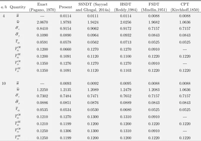
a/h Quantity Exact

(Pagano, 1970) Present

SSNDT (Sayyad and Ghugal, 2014a)

HSDT (Reddy,1984)

FSDT (Mindlin,1951)

CPT (Kirchhoff,1850)

4 u --- 0.0114 0.0111 0.0114 0.0088 0.0088

w 2.0670 1.9793 1.9424 2.0256 1.9682 1.0636

x

 _0.8410 _0.9154 _0.9062 _0.9172 _0.7157 _0.7157

y

 _0.1090 _0.0890 _0.0964 _0.0932 _0.0843 _0.0843

xy

 _0.0591 _0.0578 _0.0562 _0.0713 _0.0525 _0.0525

CR xz

 0.1200 0.0660 0.1270 0.1270 0.0910 ---

EE xz

 0.1200 0.1091 0.1120 0.1100 0.1220 0.1220

CR yz

 _0.1350 _0.1276 _0.1270 _0.1270 _0.0910 _---

EE yz

 _0.1350 _0.1091 _0.1120 _0.1103 _0.1220 _0.1220

10 u --- 0.0093 0.0092 0.0095 0.0088 0.0088

w 1.2250 1.2135 1.2089 1.2479 1.2083 1.0636

x

 _0.7302 _0.7484 _0.7471 _0.7652 _0.7157 _0.7157

y

 _0.0886 _0.0851 _0.0876 _0.0889 _0.0843 _0.0843

xy

 _0.0535 _0.0534 _0.0530 _0.0680 _0.0525 _0.0525

CR xz

 0.1210 0.1270 0.1300 0.1310 0.0910 ---

EE xz

 0.1210 0.1199 0.1200 0.1200 0.1220 0.1220

CR yz

 _0.1250 _0.1306 _0.1300 _0.1310 _0.0910 _---

EE yz

 _0.1250 _0.1199 _0.1200 _0.1200 _0.1220 _0.1220

Table 1: Comparison of non-dimensional displacements and stresses for the two layered (00_/900₎ laminated composite square (b = a) plate subjected to sinusoidally distributed load.

Figure 2: Through thickness distribution of in-plane displacement (u) for two layered (00/900) laminated composite plate subjected to sinusoidally distributed load (b = a, a/h = 10).

-0.03 -0.02 -0.01 0.00 0.01

u

-0.50 -0.25 0.00 0.25 0.50

z / h

(12)

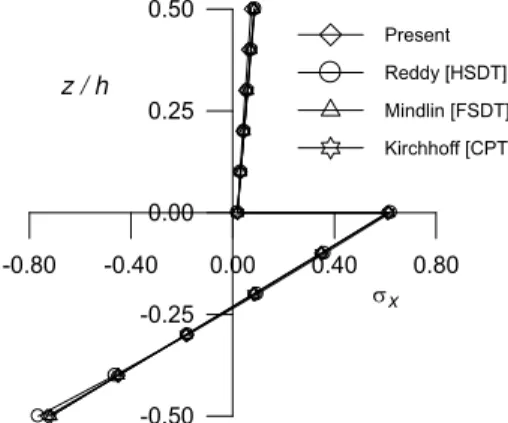
Latin American Journal of Solids and Structures 13 (2016) 516-535 Figure 3: Through thickness distribution of in-plane normal stress (x) for two layered (0

0_/900₎

laminated composite plate subjected to sinusoidally distributed load (b = a, a/h = 10).

Figure 4: Through thickness distribution of transverse shear stress ( EE xz

 ) for two layered (00/900) laminated composite plate subjected to sinusoidally distributed load (b = a, a/h = 10).

4.2 Buckling Analysis of Laminated Composite Plates

In this section, an analytical solution for the buckling analysis of plate is developed using Navier solution technique. The governing equations of the plate in case of static buckling are obtained by discarding transverse load (q) and inertia terms (I0, I1, I2, I3) from Eqs. (13) – (16). The in-plane

compressive (N ,N_xx0 0_yy andN_xy0 ) forces now represents loads instead of reaction forces, as there is no

transverse load. The values of in-plane compressive forces are taken as 0

1 0

xx

N  k N , N_yy0  k N₂ ₀and

0 ₀

xy

N  . The governing equations for static buckling are as follows:













2 2 2 3 3

0 0 0

11 2 66 2 12 66 11 3 12 66 2

3 3

11 3 12 66 2

2

2 0

b b

s s

u u v w w

A A A A B B B

x y x y x x y

w w

As As As

x x y

    

      

      

 

   

  

(32)

-0.80 -0.40 0.00 0.40 0.80 x

-0.50 -0.25 0.00 0.25 0.50

z / h

Present Reddy [HSDT] Mindlin [FSDT] Kirchhoff [CPT]

0.00 0.20 0.40

xz

-0.50 -0.25 0.00 0.25 0.50

z / h

(13)













2 2 2 3 3

0 0 0

12 66 22 2 66 2 22 3 12 66 2

3 3

22 3 12 66 2

2

2 0

b b

s s

u v v w w

A A A A B B B

x y y x y x y

w w

As As As

y x y

                            (33)

























11 12 66

2 2

22 0 1 2 2 2

4

3 3 3 3

0 0 0 0

11 3 12 66 2 22 3 12 66 2 11 4

4 4 4 4

12 66 2 2 22 4 4 2 2

4

4 0

2 2

2 2 2 2

b s b s

b

b b s s

s w w w w

k k

x y

w

u u v v

B B B B B B D

x x y y x y x

w w w w

D D D Bs Bs Bs

x y y x x y

w Bs N y            _ _                                           (34)

























11 12 66 22 12 66 11

12 66 22 11 12 66

2 2

22 0 1 2 2 2

4

3 3 3 3

0 0 0 0

3 2 3 2 4

4 4 4 4

2 2 4 4 2 2

4

4 0

2

b s b s

b

b b s s

s w w w w

Ass k k

x y

w

u

v

As

Bs

x

x y

y

x y

x

w

Bs

Ass

x y

y

x

x y

w

N

y

         _ _   













 



 





 



 







(35)

where N0 is the intensity of in-plane compressive force. After substituting Eq. (27) into Eqs. (32) –

(35), the following system of equations in matrix form is obtained.

11 12 13 14

12 22 23 24

0 2 2 2 2

13 23 33 34 1 2 1 2

2 2 2 2

14 24 34 44 1 2 1 2

0 0

0

0 0 0

0

0 0 0

0

mn

bmn

smn

u

K

v

K

N

K

k

w

K

k

w



























 



 











 



 



_

_

_

_

_

 

  

_



_

_

_

_

_

 

  



_

_

_

_

 

  



_

_

_

_

_

 

_

  

_

_{ }





(36)

where the element of stiffness matrix [Kij] are given in Eq. (29). For nontrivial solution, the determi-nant of the coefficient matrix in Eq. (36) must be zero. For each choice of m and n, there is a corresponding unique value of N0. The critical buckling load is the smallest value of N0(m, n). A

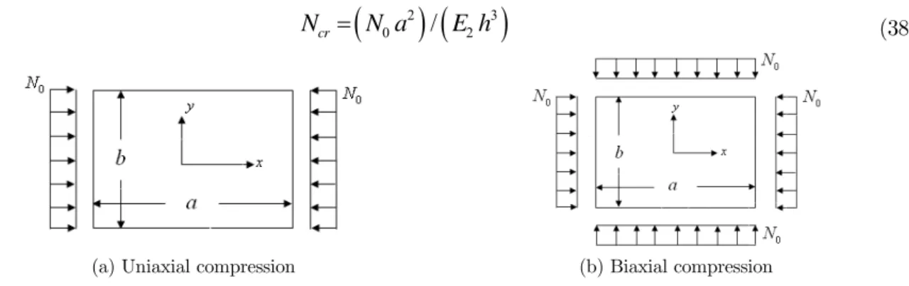
simply supported laminated composite square and rectangular plates subjected to the uniaxial and biaxial loading conditions, as shown in Figure 5, is considered to illustrate the accuracy of the present theory in predicting the buckling behaviour. The following material properties are used in the numer-ical study.

2

1 2 12 13 2 23 2 12 21 12

1

/ open, G G 0.6 , G 0.5 , 0.25, E

E E E E

E



      ₍₃₇₎

(14)



2

 

3



0

/

2

cr

N



N a

E h

₍₃₈₎

(a) Uniaxial compression (b) Biaxial compression

Figure 5: A simply supported plate subjected to in-plane compressive forces.

Layup Compression (k1, k2) Source

E1 / E2

20 30 40

(00/900/00) Uniaxial (1, 0) Present 15.215 20.428 24.977

SSNDT (Sayyad and Ghugal, 2014b) 15.003 19.002 22.330

HSDT (Reddy, 1984) 15.300 19.675 23.339

FSDT (Mindlin, 1951) 14.985 19.027 22.315

CPT (Kirchhoff, 1850) 19.712 27.936 36.160

Exact (Noor, 1975) 15.019 19.304 22.880

Biaxial (1, 1) Present 7.6075 10.214 12.488

HSDT (Reddy, 1984) 7.6500 9.8376 11.669

FSDT (Mindlin, 1951) 7.4925 9.5135 11.157

CPT (Kirchhoff, 1850) 9.8560 13.968 18.080

Exact (Noor, 1975) 7.5095 9.6520 11.440

(00/900/00/900/00) Uniaxial (1, 0) Present 16.234 21.435 25.976

HSDT (Reddy, 1984) 15.783 20.578 24.676

FSDT (Mindlin, 1951) 15.736 20.485 24.547

CPT (Kirchhoff, 1850) 19.712 27.936 36.160

Exact (Noor, 1975) 15.653 20.466 24.593

Biaxial (1, 1) Present 8.117 10.717 12.988

HSDT (Reddy, 1984) 7.8915 10.289 12.338

FSDT (Mindlin, 1951) 7.8680 10.240 12.273

CPT (Kirchhoff, 1850) 9.8560 13.968 18.080

Exact (Noor, 1975) 7.8265 10.466 12.296

(15)

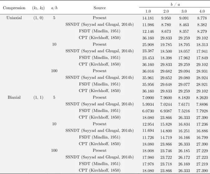
Compression (k1, k2) a/h Source b / a

1.0 2.0 3.0 4.0

Uniaxial (1, 0) 5 Present 14.181 9.950 9.091 8.778

SSNDT (Sayyad and Ghugal, 2014b) 11.986 8.780 8.463 8.382

FSDT (Mindlin, 1951) 12.146 8.673 8.357 8.279

CPT (Kirchhoff, 1850) 36.160 29.833 29.259 29.102

10 Present 25.908 19.785 18.705 18.313

FSDT (Mindlin, 1951) 23.453 18.398 17.962 17.849

CPT (Kirchhoff, 1850) 36.160 29.833 29.259 29.102

100 Present 36.016 29.682 29.094 28.931

FSDT (Mindlin, 1951) 35.956 29.648 29.077 28.921

CPT (Kirchhoff, 1850) 36.160 29.833 29.259 29.102

Biaxial (1, 1) 5 Present 7.0900 7.9600 8.1820 8.2620

FSDT (Mindlin, 1951) 6.0730 6.9387 7.5216 7.7928

CPT (Kirchhoff, 1850) 18.080 23.866 26.333 27.390

10 Present 12.954 15.828 16.834 17.236

FSDT (Mindlin, 1951) 11.726 14.719 16.166 16.799

CPT (Kirchhoff, 1850) 18.080 23.866 26.333 27.390

100 Present 18.008 23.746 26.185 27.229

FSDT (Mindlin, 1951) 17.978 23.718 26.169 27.219

CPT (Kirchhoff, 1850) 18.080 23.866 26.333 27.390

Table 3: Comparison of critical buckling load (Ncr) for simply supported four layered (00/900/900/00) laminated composite rectangular plates under uniaxial and biaxial compression.

4.3Free Vibration Analysis of Laminated Composite Plates

According to Navier solution technique, the governing equations of the plate in case of free vibration analysis are obtained by discarding transverse load (q) and in-plane compressive forces (N ,N ,N_xx0 0_yy _xy0 )

from Eq. (13) – (16). These equations are as follows:









2 2 2 3 3

0 0 0

11 2 66 2 12 66 11 3b 12 2 66 b2

u u v w w

A A A A B B B

x y x y x x y

    

      

      





3 3 2

0

11 3s 12 2 66 s2 0 2 0

w w u

As As As I

x x y t

  

    

   

(16)













2 2 2 3 3

0 0 0

12 66 22 2 66 2 22 3 12 66 2

3 3 2

0

22 3 12 66 2 0 2

2

2 0

b b

s s

u v v w w

A A A A B B B

x y y x y x y

w w v

As As As I

y x y t

                               (40)













11



12 66



2 2 4 4

22 0 2 2 1 2 2 2 2

4

3 3 3 3

0 0 0 0

11 3 12 66 2 22 3 12 66 2 11 4

4 4 4 4

12 66 2 2 22 4 4 2 2

4 4

2 2

2 2 2 2

b s b b

b

b b s s

s w w w w

I I

t t x t y t

w

u u v v

B B B B B B D

x x y y x y x

w w w w

D D D Bs Bs Bs

x y y x x y

w Bs y         _  _ _  _                                                 4 4

2 2 2 2 2 0

s s

w w

I

x t y t

     _  _       (41)

















11 12 66 22 12 66 11

12 66 22 11 12 66

2 2 4 4

22 0 2 2 2 2 2

4

3 3 3 3

0 0 0 0

3 2 3 2 4

4 4 4 4

2 2 4 4 2 2

4 4

2 2

2 2 2 2

b s b

b

b b s s

s w w w

Ass I I

t t x t

w

u u v v

As As As As As As Bs

x x y y x y x

w w w w

Bs Bs Bs Ass Ass Ass

x y y x x y

w y       _  _                                              4 4 3

2 b2 2 s2 2 s2 0

w w w

I

y t x t y t

     

 

 _{ }  _{ } _{ } 

   

(42)

The following solution form is assumed for unknown displacement variables

u

₀,

v

₀,

w

band

w

s

0

1 3 5 1 3 5

cos

sin

cos

sin

mn

m , , n , ,

b bmn

s smn

u

x

y

t

v

x

y

t

w

x

y

t

w

x

y

t

























   

 





 



 

_



 





 



 



 





 

(43)

Substituting Eq. (43) into the Eqs. (39) – (42), the following system of equations is obtained.

11 12 13 14 0

12 22 23 24 2 0

2 2 2 2

13 23 33 34 1 0 2 0

2 2 2 2

14 24 34 44 2 0 3 0

0 0 0 0

0 0 0

mn mn bmn smn

u

K K K K I

v

K K K K I

K K K K I ( ) I I ( ) I w

                         _ __ _ _    _ _ _ _ _ _ _ _ _     _ _ _ _     _ _ _     _{ }    _ _{ }   (44)

The elements of stiffness matrix [K] are given in Eq. (29). From the solution of Eq. (44) lowest natural frequencies for laminated composite plates can be obtained. The material properties given by Eq. (37) are used for the numerical study. Natural frequencies are presented in the following non-dimensional form:

2 2

/

h

E

(17)

Lay-up Source E1 / E2

10 20 30 40

00/900 Present 0.27987 0.31354 0.34128 0.36498

SSNDT (Sayyad and Ghugal, 2015) 0.28060 0.31415 0.34181 0.36543

HSDT (Reddy, 1984) 0.27955 0.31284 0.34020 0.36348

FSDT (Mindlin, 1951) 0.27757 0.30824 0.33284 0.35353

CPT (Kirchhoff, 1850) 0.30968 0.35422 0.39335 0.42884

Exact (Noor, 1973) 0.27938 0.30698 0.32705 0.34250

00/900/00 Present 0.34261 0.40623 0.44502 0.47162

HSDT(Reddy, 1984) 0.33095 0.38112 0.41094 0.43155

FSDT (Mindlin, 1951) 0.32739 0.37110 0.39540 0.41158

CPT (Kirchhoff, 1850) 0.42599 0.55793 0.66419 0.75565

Exact (Noor, 1973) 0.32841 0.38241 0.41089 0.43006

00/900/900/00 Present 0.3422 0.4055 0.4441 0.4706

HSDT(Reddy, 1984) 0.3308 0.3810 0.4108 0.4314

FSDT (Mindlin, 1951) 0.3319 0.3826 0.4130 0.4341

CPT (Kirchhoff, 1850) 0.4260 0.5579 0.6642 0.7556

Exact (Noor, 1973) 0.3284 0.3824 0.4108 0.4300

00_/900_/00_/900_/00 _Present _0.3430 _0.4063 _0.4449 _0.4715

HSDT(Reddy, 1984) 0.3399 0.3994 0.4350 0.4592

FSDT (Mindlin, 1951) 0.3368 0.3930 0.4271 0.4506

CPT (Kirchhoff, 1850) 0.4259 0.5579 0.6641 0.7556

Exact (Noor, 1973) 0.3408 0.3979 0.4314 0.4537

Table 4: Comparison of non-dimensional natural frequencies of simply supported square laminated composite plates (b = a, a/h = 5).

5 DISCUSSION OF NUMERICAL RESULTS

5.1 Bending Analysis of Laminated Composite Plates

(18)

theories for aspect ratio 10. Figure 3 shows that, in-plane normal stress

 

x predicted by present

theory is in close agreement with that of other theories. The present theory predicts exact values of transverse shear stress

 

xz for aspect ratios 4 and 10 when obtained via equations of equilibrium

 

EE xz

 . Through thickness distribution of this stress is shown in Figure 4.

5.2 Buckling Analysis of Laminated Composite Plates

A comparison of the critical buckling load parameters obtained by the present theory for a three layered (00/900/00) and five layered (00/900/00/900/00) symmetric cross-ply laminated composite square plates subjected to uniaxial and biaxial compressions for various modular ratios (E1/E2) is

presented in Table 2. All the layers are of equal thickness. The results of present theory are compared with HSDT of Reddy (1984), SSNDT of Sayyad and Ghugal (2014b) FSDT of Mindlin (1951) and CPT of Kirchhoff (1850) and exact elasticity solution given by Noor (1975). The material properties used for this example are shown in Eq. (37). From the examination of Table 2 it is observed that the present results are in excellent agreement with exact solution as well as HSDT of Reddy (1984). It is also observed that the buckling loads predicted by CPT are significantly higher than those obtained by the present theory. This is the consequence of neglecting the transverse shear deformation effect in the CPT. It can be seen from Table 2 that the critical buckling loads in case of biaxial compression are exactly half of those of uniaxial compression for square plates. Table 3 shows the critical buckling load parameter for four layered (00/900/900/00) symmetric laminated composite rectangular plate. The numerical results are obtained for various values of b/a ratios and a/h ratios. From Table 3 it is observed that the critical buckling load increases with respect to increase in ‘b/a’ and ‘a/h’ ratios. It is also pointed out that the present theory is in excellent agreement while predicting the buckling behaviour of rectangular laminated composite plates.

5.3 Free Vibration Analysis of Laminated Composite Plates

In Table 4, non-dimensional natural frequencies of simply supported square laminated composite plates for various modular ratios (E1/E2) are presented and compared with those obtained by SSNDT

of Sayyad and Ghugal (2015), HSDT of Reddy (1984), FSDT of Mindlin (1951) and CPT of Kirchhoff (1850). In all the lamination schemes, the layers are of equal thickness. The material properties are shown in Equation (37). The exact elasticity solution for free vibration analysis of laminated compo-site plates given by Noor (1973) is used for the purpose of comparison. From the Table 8 it is observed that the present theory is in excellent agreement while predicting the natural frequencies of laminated composite plates. The CPT overestimates the natural frequencies because of neglect of the transverse shear deformation effect. It is also observed that the natural frequencies of laminated composite plates increase with respect to increase in modular ratios (E1/E2).

6 CONCLUSIONS

(19)

deformation theory and other higher order theories. The present theory satisfies the traction free conditions at top and bottom surfaces of plates without using shear correction factor. From the mathematical formulation of present theory, it is observed that, due to four unknown variables, the present theory requires less computational efforts compared to five and six variable shear deformation theories. From the numerical results and discussion it is concluded that present theory is in good agreement while predicting the bending, buckling and free vibration behaviour of laminated composite plates.

References

Ameur, M., Tounsi, A., Mechab, I. and Bedia, E.A.A., (2011). A new trigonometric shear deformation theory for bending analysis of functionally graded plate resting on elastic foundation, KSCE J. of Civil Engineering, 15:1405-1414.

Daouadji, T.H., Tounsi, A., Hadji, L., Henni, A.H. and Bedia, E.A.A., (2012). A theoretical analysis for static and dynamic behavior of functionally graded plates, Material Physics and Mechanics, 14:110-128.

Daouadji, T.H., Tounsi, A. and Bedia, E.A.A., (2013). A new higher order shear deformation model for static behavior of functionally graded plates, Advances in Applied Mathematics and Mechanics, 5:351-364.

Ghugal, Y.M. and Sayyad, A.S., (2010). A static flexure of thick isotropic plates using trigonometric shear deformation theory, J. of Solid Mechanics, 2:79–90.

Ghugal, Y.M. and Sayyad, A.S., (2013a). Static flexure of thick orthotropic plates using trigonometric shear defor-mation theory, J. of Structural Engineering, (India) 39:512–521.

Ghugal, Y.M. and Sayyad, A.S., (2013b). Stress analysis of thick laminated plates using trigonometric shear defor-mation theory, Int. J. of Applied Mechanics, 5:1–23.

Jones, R.M. 1975. Mechanics of Composite Materials, Tokyo: McGraw Hill Kogakusha Ltd.

Karama, M., Afaq, K.S. and Mistou, S., (2009). A new theory for laminated composite plates, Proc. IMechE Part L: J. Materials: Design and Applications, 223:53-62.

Kim, S.E., Thai, H.T. and Lee, J., (2009). Buckling analysis of plates using the two variable refined plate theory, Thin Walled Structure, 47:455–462.

Kirchhoff, G.R., (1850). Uber das gleichgewicht und die bewegung einer elastischen Scheibe, J. für die Reine und Angewandte Mathematik (Crelle's Journal), 40: 51-88.

Meiche, N.E., Tounsi, A., Ziane, N., Mechab, I. and Bedia, E.A.A., (2011). New hyperbolic shear deformation theory for buckling and vibration of functionally graded sandwich plate, Int. J. of Mechanical Sciences, 53:237–247.

Metin, A., (2009). A new shear deformation theory for laminated composite plates, Composite Structures, 89:94–101. Mindlin, R.D., (1951). Influence of rotatory inertia and shear on flexural motions of isotropic, elastic plates, ASME J. of Applied Mechanics,18: 31-38.

Noor, A.K., (1973). Free vibrations of multilayered composite plates, AIAA J.11:1038-1039.

Noor, A.K., (1975). Stability of multilayered composite plates, Fibre Science and Technology, 8:2 81-89.

Pagano, N.J., (1970). Exact solutions for bidirectional composites and sandwich plates, J. of Composite Materials,

4:20-34.

Reddy, J.N., (1984). A simple higher order theory for laminated composite plates, ASME J. of Applied Mechanics, 51: 745–752.