Mode Shape Analysis of Multiple Cracked
Functionally Graded Timoshenko Beams
1 INTRODUCTION
Since the FGMs are increasingly implemented in the practice of industries, dynamics of cracked structures made of FGM gets an enormous attention of researches and engineers. Also, a number of methods has been proposed to vibration analysis of the structures such as Galerkin’s method, Finite Element Method (FEM), Dynamic Stifness Method (DSM), … However, for the simple structures such as beams the analytical approach shows to be most accurate and efficient. Yan et al. (2008) calculated natural frequencies and mode shapes of cracked FGM Euler-Bernoulli beam. Ke et al. (2009) studied effects of open edge cracks to vibration of FGM Timoshenko beam with different
Tran Van Lien a, * Ngo Trong Đuc b Nguyen Tien Khiem c
a National University of Civil
Engineering; [email protected]
b Design Consultant and Investment of
Construction, [email protected].
c Institute of Mechanics, Vietnam
Academy of Science and Technology, [email protected].
* Corresponding author
http://dx.doi.org/10.1590/1679-78253496
Received 07.11.2016 In revised form 14.05.2017 Accepted 15.05.2017 Available online 26.05.2017 Abstract
The present paper addresses free vibration of multiple cracked Ti-moshenko beams made of Functionally Graded Material (FGM). Cracks are modeled by rotational spring of stiffness calculated from the crack depth and material properties vary according to the power law throughout the beam thickness. Governing equations for free vi-bration of the beam are formulated with taking into account actual position of the neutral plane. The obtained frequency equation and mode shapes are used for analysis of the beam mode shapes in de-pendence on the material and crack parameters. Numerical results validate usefulness of the proposed herein theory and show that mode shapes are good indication for detecting multiple cracks in Timo-shenko FGM beams.
Keywords
boundary conditions. Aydin (2013) established frequency equations of free vibration for FGM Euler-Bernoulli beam with arbitrary number of cracks. Likely, the authors (J. Yang, Y. Chen, Y. Xiang, X.L. Jia 2008; J. Yang, Y. Chen 2008) obtained frequency equation of the beam in the form of third order determinant without using transfer matrix method at crack positions. Wei et al. (2012) estab-lished equations of motion of FGM Timoshenko beam with rotary inertia and shear deformation included. Because of ignoring axial inertia, the bending vibration is independent from axial vibration. The authors used transfer matrix method to obtain frequency equations and mode shapes of beam with arbitrary number of open edge cracks only in the form of third-order determinant. This is re-markable achievement in free vibration amalysis of multiple cracked FGM beam. Sherafatnia et al. (2014) analyzed natural frequencies and mode shapes of cracked beam using different theories of beam. It was demonstrated by the authors that fundamental mode shape is the same for all the beam theories, but notable difference between the mode shapes is revealed for the higher modes.
Using Galerkin’s procedure, Yan et al. (2011) obtained dynamic deflections of cracked FGM beam on elastic foundation under a transverse moving load. Kitipornchai et al. (2009) used Ritz’s method to analyze nonlinear vibration of an open edge crack FGM Timoshenko beam. Wattanasakulpong et al. (2012) investigated free vibration of FGM beams with general elastically end constraints by dif-ferential transformation method. The FEM has been used to calculate frequencies and mode shapes of FGM beam (Z.G. Yu, F.L. Chu 2009; S.D. Akbas 2013; A. Banerjee, B. Panigrahi, G. Pohit 2015). As the FEM is formulated by using frequency independent polynomial shape function, this method cannot capture all necessary high frequencies of interest. This limitation of the FEM could be resolved by using DSM (H. Su, A. Banerjee 2015; N.T. Khiem, N.D. Kien, N.N. Huyen 2014; T.V. Lien, N.T. Duc and N.T. Khiem 2016; N.T. Khiem, T.V. Lien 2002). Since the dynamic stiffness method uses the frequency-dependent shape functions obtained from the exact solution of the governing differential equations of free vibration, natural frequencies and mode shapes obtained by the method should be more accurate. Nevertheless, there is very little effort devoted to develop the DSM for vibration analysis of cracked FGM Timoshenko beams.
On the other hand, because of grading material properties the neutral plane and mid plane of the FGM beams are different and effect of the neutral plane position on static and dynamic behavior of the beam is investigated in some studies. Eltaher et al. (2013) showed that the natural frequencies calculated by using the mid-plane theory of FGM beam are higher than those obtained by taking into account actual position of neutral plane. Furthermore, study by Huyen and Khiem (2016) revealed that taking into account actual position of neutral plane simplifies the governing differential equations of FGM beam and allows one to find a condition for uncoupling of axial and flexural vibrations likely to the homogeneous beam.
2 GOVERNING EQUATIONS
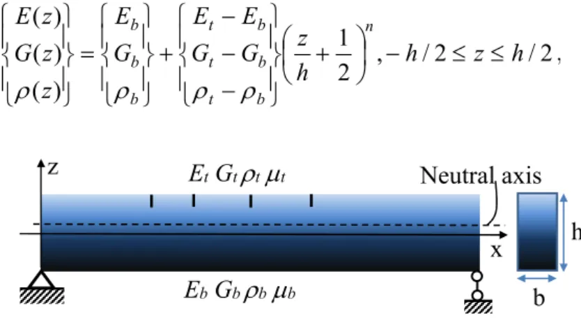
Consider a FGM beam of length L, cross sectional area A=b×h. It is assumed that the material properties of FGM beam vary along the thickness direction by the power law distribution as follows
2
/
2
/
,
2
1
)
(
)
(
)
(
h
z
h
h
z
G
G
E
E
G
E
z
z
G
z
E
nb t
b t
b t
b b b
, (1)
Figure 1: A multiple cracked FGM beam.
where E, G and ρ stand for Young’s, shear modulus and material density, n is power law exponent, z is co-ordinate of point from the mid plane at high h/2 (Fig. 1). Based on the Hamilton’s principle, we can get free vibration equations of FGM Timoshenko beam in frequency domain in the form (T.V. Lien, N.T. Duc and N.T. Khiem 2016)
0
~
~
~
z
Π
z
C
z
A
(2)where T
W
U
,
,
}
{
z
is amplitude of axial displacement, rotationand deflection
W
u
x
t
x
t
w
x
t
e
dt
U
,
,
}
{
(
,
),
(
,
),
(
,
)}
it{
0 0 (3)and matrices (see Appendix A1)
11 2 33 22 2 12
2 12
2 11
2
33 33 33
22 12
12 11
0
0
0
0
)
(
~
;
0
0
0
0
0
0
0
~
;
0
0
0
0
~
I
A
I
I
I
I
A
A
A
A
A
A
A
C
Π
A
(4)Seeking solution of equation (2) in the form x
e
d
z
0
, we obtain so-called characteristic equation0
]
~
~
~
det[
2A
Π
C
(5) This is a cubic algebraic equation respect to=2 that can be elementarily solved and gives three roots 1,2,3 (
see Appendix A2).
Therefore, we get3
,
2
,1
,
;
;
;
2,5 2 3,6 3 14 ,
1
k
k
k
k
j
jj
(6)b
h
x
z
E
tG
t
t
tNeutral axis
General continuous solution of Eq. (2) can be now represented as
x xe
e
d
d
d
d
d
d
d
d
d
6 1 36 32 31 26 22 21 16 12 11 0...
...
...
z
(7)Taking into account the first and last equations in (2) one gets
11 12 16 1 1 2 2 6 6
21 22 26 1 2 6
31 32 36 1 1 2 2 6 6
...
...
...
...
...
...
d
d
d
C
C
C
d
d
d
C
C
C
d
d
d
C
C
C
where
C
1,...,
C
6 are constants and6
,...,
2
,1
;
)
(
;
33 2 11 2 33 11 2 11 2 12 2
j
A
I
A
A
I
I
j j j jj
.Using the notations introduced in (6) it is easily to verify that
3 6 2 5 1 4 3 6 2 5 1
4
;
;
;
;
;
.Therefore, expression (7) can be now rewritten in the form
C
G
z
0(
x
,
)
(
x
,
)
, (8)where T
C
C
,...,
)
(
1 6
C
andG
(
x
,
)
[
G
1(
x
,
)
G
2(
x
,
)]
are function matrices
x k x k x k x k x k x k x k x k x k x k x k x k x k x k x k x k x k x ke
e
e
e
e
e
e
e
e
x
e
e
e
e
e
e
e
e
e
x
3 2 1 3 2 1 3 2 1 3 2 1 3 2 1 3 2 1 3 2 1 3 2 1 2 3 2 1 3 2 11
(
,
)
;
(
,
)
G
G
(9)It is assumed that the beam has been cracked at different positions
e
1,...,
e
n. Based on fracture mechanics (F. Erdogan, B.H. Wu 1997), the stiffness reduction of FGM beam caused by presence of the cracks can be modeled by equivalent springs of stiffness Kj (Ke et al., 2009). Therefore, conditionsthat must be satisfied at the cracks are (T.V. Lien, N.T. Duc and N.T. Khiem 2016)
)
(
)
0
(
)
0
(
);
0
(
)
0
(
);
0
(
)
0
(
)
(
)
0
(
)
0
(
;
/
)
(
)
0
(
)
0
(
);
0
(
)
0
(
j j j j j j j j j j j j j j j je
M
e
M
e
M
e
Q
e
Q
e
N
e
N
e
N
e
W
e
W
K
e
M
e
e
e
U
e
U
(10)where N, Q and M are internal axial, shear forces and bending moment respectively (N.T. Khiem, N.D. Kien, N.N. Huyen 2014)
)
(
;
;
12 22 3312
11
A
U
xA
M
A
U
xA
xQ
A
W
xSubstituting (11) into (10), one can rewrite the conditions (10) as follows
n
j
K
A
e
e
W
e
W
e
e
e
U
e
U
e
W
e
W
e
e
e
e
U
e
U
j j j x j j x j x j x j x j x j x j j j x j j j j j,...,
3
,
2
,1
;
/
)
(
)
0
(
)
0
(
);
0
(
)
0
(
);
0
(
)
0
(
)
0
(
)
0
(
);
(
)
0
(
)
0
(
);
0
(
)
0
(
22
(12)So called crack magnitudes j defined in (12) are function of the material properties such as
Young’s modulus, power law exponent n and cross sectional dimensions. For the FGM beam, the crack magnitude can be calculated as
2 2 3 2)
1
(
)
2
(
2
)
3
(
3
3
12
)
,
(
;
12
/
;
/
)
,
(
n
n
R
n
n
R
n
n
R
n
R
bh
I
R
I
E
n
R
E E E E b b E b j (13)In case of homogenous beam Et=Eb=E0 (RE=1), the crack magnitudes can be calculated from
crack depth aj as
)
6
.
19
7556
.
40
1063
.
47
0351
.
33
2948
.
20
9736
.
9
5948
.
4
04533
.
1
6272
.
0
(
)
(
;
)
(
.
).
1
(
6
/
8 7 6 5 4 3 2 2 2 0 0 0z
z
z
z
z
z
z
z
z
z
f
h
a
z
z
f
h
R
I
E
j j
(14)Therefore, for modal analysis of cracked FGM beam, the crack magnitudes can be approximated by (Khiem and Huyen 2016)
)
(
)
,
(
.
).
1
.(
6
)
(
z
2h
2R
n
f
z
F
Ej
(15)These functions would be used below for determining spring stiffness from given crack depth. First, seeking solution
S
( )
x
of equation (2) satisfying the conditionsT T
;
(
0
)
(
0
,
0
,
1
)
)
0
,1
,
0
(
)
0
(
S
S
(16)one finds
{ , , }
1 2 3 TS S S
S
where (T.V. Lien, N.T. Duc and N.T. Khiem 2016)x
k
x
k
x
k
x
S
x
k
x
k
x
k
x
S
x
k
x
k
x
k
x
S
3 3 3 2 2 2 1 1 1 3 3 3 3 2 2 2 1 1 1 2 3 3 2 2 1 1 1sinh
sinh
sinh
)
(
cosh
cosh
cosh
)
(
cosh
cosh
cosh
)
(
(17)
1 2 2 3 3
3 2 2 3 3 1 1 1 33 1 1 2 2 2 1 1 1 3 2 2 2 1 3 3 3 2 1
(
) / ;
(
) / ;
(
) / ;
(
)
(
)
(
).
k
k
k
k
k
k
k
k
k
(18)1 1
( )
( )
( ) (
),
j
x
jx
j
je
jx e
jz
z
S
(19)where
z
j1(
x
)
is solution in(
e
j1,
e
j)
being continuously expended to the subsequent interval)
,
(
e
je
j1 andS
( )
x
is defined in the form (17). Namely, since both functionsz
j1(
x
)
,S
(
x
e
j)
aresolutions of Eq. (2) in
(
e
j,
e
j1)
, their combination in (19) would be solution of that equation in theinterval. Moreover, solution (19) satisfies also the conditions
)
(
)
(
)
(
);
(
)
(
);
(
)
(
)
(
)
(
);
(
)
(
)
(
);
(
)
(
1 1 1 1 1 1 1 j j j j j j j j j j j j j j j j j j j j j j j j j j j j j je
e
W
e
W
e
e
e
U
e
U
e
W
e
W
e
e
e
e
U
e
U
(20)These conditions ensure that solution of Eq. (2) in the form of (19) satisfy condition at crack positions (12). Based on the recurrent connection, one can express general solution of Eq. (2) for FGM beam with n crack in the form
n
j
e
e
S
e
e
x
x
x
j k k j k j j j n j j j c,...,
3
,
2
,1
,
)
(
)
(
)
(
)
(
)
(
1 1 2 0 1 0
K
z
z
(21)In the later equation,
z
0(
x
)
is continuous solution found above in the form (7) and function K(x) is
0
for
)
(
0
for
0
)
(
;
0
for
)
(
0
for
0
)
(
x
x
x
x
x
x
x
x
S
K
S
K
(22)Suppose that boundary conditions for solution of Eq. (2), are represented by
00
;
L
0
0
z
x
B
z
xL
B
(23)where B0, BL are differential matrix operators of dimension 3×3 given in
Appendix A3
. Since thesecond term of solution (21) satisfy any trivial condition at
x
0
,the first condition in (23) is
only
applied for
z
0(
x
)
. Splitting the constant vector{
,
}
T2 1
C
C
C
intoT T
C
C
C
C
C
C
,
,
}
;
{
,
,
}
{
1 2 3 2 4 5 61
C
C
, the boundary condition at the left end of the beam can berewritten as
1
0 02 0
2
00 01 2 02 1 01
)
,
(
)
(
;
)
,
(
)
(
0
x xx
x
B
G
B
B
G
B
C
B
C
B
(24)Eq. (24) allows eliminating one of the vectors
C
1,
C
2 and as result the solutionz
0(
x
)
can be reassembled asz
0(
x
,
)
G
0(
x
,
)
D
withG
0(
x
,
)
is 3×3 dimension matrix function andarbi-trary constant vector T
D
D
D
,
,
}
{
1 2 3
]
)
,
(
)
,
(
)
,
(
[
)
(
21 1 22 2 23 30
x
g
x
D
g
x
D
g
x
D
(25)where
g
2k(
x
,
),
k
,1
2
,
3
are elements on second row of matrixG
0(
x
,
)
. So, solution (20) can be now expressed as
nj
j j
c
x
x
x
e
1
0
(
,
)
(
)
)
(
G
D
K
z
(26)Satisfying boundary condition at right end of the beam leads to
x L c j L
j
x L nj
j j L
e
x
e
x
e
)
(
)
(
;
)
,
(
)
(
0
)}
(
{
}
)]{
(
[
0 0
1 0
S
B
b
G
B
B
b
D
B
L
L
(27)
In the case of intact beam, when
μ
j
0
,
j
1
,...,
n
, equation (27) is reduced to0
}
)]{
(
[
B
L0
D
(28)that enables to determine undamaged natural frequencies by solving the equation
0
)]
(
det[
)
(
00
L
L
B
(29)Each roots
0j of this equation is related to mode shapej j j
j
(
x
)
C
G
(
x
,
)
D
0 0 00
(30)where
C
0j is an arbitrary constant andD
j is the normalized solution of (28) corresponding to
0j .For cracked beam, the constant vector D is sought in the form
nj
j j
1
D
D
that leads theequation (27) to
[
B
L0(
)]{
D
j}
{
b
c(
e
j)}
from that one is able to calculate)}
(
){
/
1
(
)}
(
{
)]
(
[
L0 1 c j 0 c jj
B
b
e
L
b
e
D
(31) Therefore, solution (26) gets the form
nj
j c j
j
c
x
L
L
x
e
x
e
1 0 0
0
)
[
(
)
(
)
(
,
)
(
)]
/
1
(
)
(
K
G
b
z
(32))
(
)
,
(
)
(
)
,
(
)
(
)
,
(
,...,
3
,
2
,1
],
)
(
)
(
[
)
/
(
3 23
2 22
1 21
2 0 1 0
k c j k
c j k
c j jk
jk k j n
k k j
j
e
b
e
g
e
b
e
g
e
b
e
g
g
n
j
g
e
e
K
L
L
The above equation can be rewritten in the matrix form
T n T
n T
n
jk k j jk
n
e
e
n
k
j
g
e
e
K
L
a
diag
L
}
,...,
{
;
}
,...,
{
;
}
,...,
{
]
,...,
2
,1
,
;
)
(
).
(
[
)
,
(
};
,...,
{
)
(
0
}
)]{
,
(
)
(
)
(
[
1 1
1
2 0
1
0
e
γ
μ
e
A
γ
μ
e
A
γ
I
(33)
Condition for existence of non-trivial solution of Eq. (33) is
0
)]
,
(
)
(
)
(
det[
)
,
,
(
γ
e
L
0
I
γ
A
e
f
(34)This is frequency equation for FGM beam with arbitrary number of cracks, solution of which gives natural frequencies (j, j=1,2,3,..). In particularity, when vector = 0, Eq. (34) becomes Eq.
(29).
Once a natural frequency has been found, we can determine vector j from the Eq. (33) as an
eigenvector T
jn j
j
{
1,...,
}
μ
that enables to determine mode shape related to the natural fre-quency j as
nk
k c j k
j jk j
j
L
x
e
x
e
L
x
1 0 0
0
)]
(
)
,
(
)
(
)
(
[
)
(
1
)
(
K
G
b
Φ
(35)Since the eigenvector jis determined with an arbitrary constant that could be specified by using
a normality condition, for instance
(
)
1
max
Φ
jx
(36)3 ANALYSIS OF MODE SHAPES OF MULTIPLE CRACKED FGM TIMOSHENKO BEAM
3.1 Comparison in Particular Cases
For validation of the obtained above equations in this subsection we compare natural frequencies and mode shapes computed by the equations (33) and (35) with those obtained by using other methods in the cases of homogeneous beam and uncracked FGM beam.
Natural frequencies and mode shapes of three lowest modes computed for the beam and compared to those obtained by Lien and Hao (2013) are shown in Table 1 and Fig. 2. It is easily to see a good agreement of the obtained results.
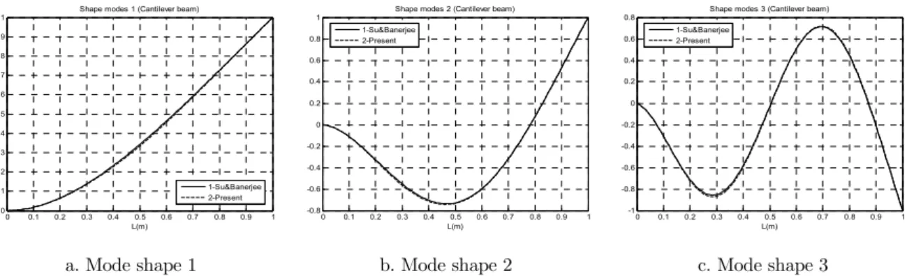
b)Intact FGM beam: An intact cantilever FGM Timoshenko beam with aluminum Al2O3 in the
top: Et=390GPa, t=3960kg/m3, t=0.25 and steel at the bottom: Eb=210GPa, b=7800kg/m3, b=0.31 is examined for power law exponent n=1 and geometry dimensions L=1.0m, b=0.1m,
h=0.1m (H. Su, J.R. Banerjee 2015).
Three lowest frequencies and mode shapes of the FGM beam obtained by using the presented above theory are compared with those given in H. Su, J.R. Banerjee (2015) and illustrated in Table 1 and Fig. 3. It can be observed that the calculated results are very close to the results of Su & Banerjee (2015).
a. Mode shape 1 b. Mode shape 2 c. Mode shape 3
Figure 2: Comparison of three lowest mode shapes for simple support Timoshenko beam with 2 cracks at position 0.2m and 0.4m, crack depth a/h=30%.
a. Mode shape 1 b. Mode shape 2 c. Mode shape 3
Figure 3: Comparison of the first three mode shapes with Su & Banerjee (2015) for intact cantilever FGM Timoshenko beam.
0 0.1 0.2 0.3 0.4 0.5 0.6 0.7 0.8 0.9 1 -1
-0.9 -0.8 -0.7 -0.6 -0.5 -0.4 -0.3 -0.2 -0.1 0
L(m) Shape modes 1 (Simply support beam)
1-Lien&Hao 2-Present
0 0.1 0.2 0.3 0.4 0.5 0.6 0.7 0.8 0.9 1 -1
-0.8 -0.6 -0.4 -0.2 0 0.2 0.4 0.6 0.8 1
L(m) Shape modes 2 (Simply support beam)
1-Lien&Hao 2-Present
0 0.1 0.2 0.3 0.4 0.5 0.6 0.7 0.8 0.9 1 -1
-0.8 -0.6 -0.4 -0.2 0 0.2 0.4 0.6 0.8 1
L(m) Shape modes 3 (Simply support beam)
1-Lien&Hao 2-Present
0 0.1 0.2 0.3 0.4 0.5 0.6 0.7 0.8 0.9 1 0
0.1 0.2 0.3 0.4 0.5 0.6 0.7 0.8 0.9 1
L(m) Shape modes 1 (Cantilever beam)
1-Su&Banerjee 2-Present
0 0.1 0.2 0.3 0.4 0.5 0.6 0.7 0.8 0.9 1 -0.8
-0.6 -0.4 -0.2 0 0.2 0.4 0.6 0.8 1
L(m) Shape modes 2 (Cantilever beam) 1-Su&Banerjee
2-Present
0 0.1 0.2 0.3 0.4 0.5 0.6 0.7 0.8 0.9 1 -1
-0.8 -0.6 -0.4 -0.2 0 0.2 0.4 0.6 0.8
L(m) Shape modes 3 (Cantilever beam) 1-Su&Banerjee
Figs Cases Freq. 1 (rad/s) Freq. 2 (rad/s) Freq. 3 (rad/s)
2 Present 1316.9 5131.4 10743 Lien & Hao 1330.7 5162.5 10803
3 Present 708.5 4248.7 11086 Su & Banerjee 719.0 4314.0 11220
4
0 crack 990.53 3782.6 7963.2 1 crack 972.22 3584.8 7464.5 2 cracks 919.77 3403.7 7463.9 3 cracks 856.15 3402.4 7016.1 4 cracks 808.42 3274.1 6971.5 5 cracks 785.25 3073.8 6662.5 6 cracks 781.0 3016.6 6439.2
5
a/h=0% 990.53 3782.6 7963.2 a/h=10% 973.11 3758.3 7918.2 a/h=20% 927.29 3689.6 7806.4 a/h=30% 858.76 3572.1 7656.0 a/h=40% 771.73 3393.3 7491.0 a/h=50% 669.14 3131.8 7328.9
6
a/h=10% 987.12 3751.1 7903.8 a/h=20% 977.39 3664.6 7752.3 a/h=30% 960.34 3526.3 7540.6
7
a/h=10% 2141.4 5472.1 9855.6 a/h=20% 2140.5 5430.4 9702.7 a/h=30% 2139.0 5365.0 9481.5
8
a/h=10% 352.26 2131.6 5548.5 a/h=20% 342.07 2131.3 5502.9 a/h=30% 325.72 2130.8 5418.2
9
a/h=10% 966.69 3697.1 7798.0 a/h=20% 906.19 3478.2 7367.6 a/h=30% 820.88 3165.0 6736.2
10
a/h=10% 2120.6 5417.1 9758.9 a/h=20% 2064.6 5237.8 9357.3 a/h=30% 1979.2 4982.5 8781.0
11
a/h=10% 350.39 2095.6 5477.2 a/h=20% 335.52 2002.4 5234.9 a/h=30% 312.86 1866.2 4874.6
12
1 crack 960.34 3526.3 7540.6 2 cracks 892.98 3478.9 7256.2 3 cracks 839.06 3353.7 7185.8 4 cracks 820.88 3165.0 6736.2
13
1 crack 2139.0 5365.0 9481.5 2 cracks 2052.0 5247.7 9229.8 3 cracks 1987.4 5054.7 9181.3 4 cracks 1979.2 4982.5 8781.0
14
1 crack 325.72 2130.8 5418.2 2 cracks 315.48 2014.1 5297.4 3 cracks 313.05 1889.2 5093.8 4 cracks 312.86 1866.2 4874.6
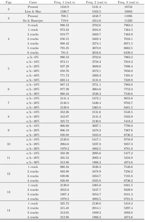
3.2 Change in Mode Shapes of Multiple Cracked FGM Timoshenko Beam
a. Mode shape 1 b. Mode shape 2 c. Mode shape 3
Figure 4: Change in first three mode shapes of simple support FGM Timoshenko beam which has 0 to 6 equidistant cracks (=0.15m) of the same depth a/h=30%.
a. Mode shape 1 b. Mode shape 2 c. Mode shape 3
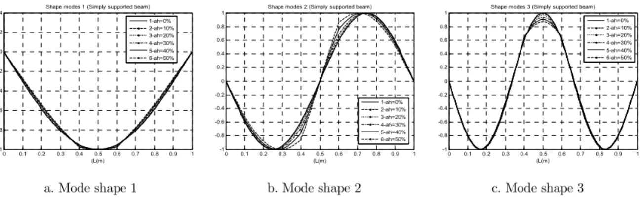
Figure 5: Change in first three mode shapes of simple support FGM beam with 2 cracks at 0.4m and 0.6m and depth varying from a/h=0% to 50%.
In this section, the cracked FGM beam of material properties: Et=70GPa, t=2780kg/m3, t=0.33,
Eb/Et=0.5; b=7850kg/m3, b=0.33, n=0.5 and geometric parameters: L=1.0m, b=0.1m, h=0.1m is
investigated. Three lowest mode shapes of a simply supported FGM Timoshenko beam with various number (from 0 to 6) equidistant cracks of the same depth a/h=30% are shown in Fig. 4 and the mode shapes in case of 2 cracks (at 0.4m and 0.6m) with equal depth varying from 0% to 50% are presented in Fig. 5. It is observed variation of the mode shapes caused by number of cracks and their depth. However, location of the cracks is difficult to detect by observing only the mode shape graphs, it could be identified by comparison with mode shapes of uncracked beam that is demonstrated in the subsequent Figures.
0 0.1 0.2 0.3 0.4 0.5 0.6 0.7 0.8 0.9 1 -1
-0.8 -0.6 -0.4 -0.2 0 0.2
0.4 Shape modes 1 (Simply supported beam)
(L(m)
1-0crack 2-1crack 3-2cracks 4-3cracks 5-4cracks 6-5cracks 7-6cracks
0 0.1 0.2 0.3 0.4 0.5 0.6 0.7 0.8 0.9 1 -1
-0.8 -0.6 -0.4 -0.2 0 0.2 0.4 0.6 0.8
1 Shape modes 2 (Simply supported beam)
(L(m)
1-0crack 2-1crack 3-2cracks 4-3cracks 5-4cracks 6-5cracks 7-6cracks
0 0.1 0.2 0.3 0.4 0.5 0.6 0.7 0.8 0.9 1 -1
-0.8 -0.6 -0.4 -0.2 0 0.2 0.4 0.6 0.8
1 Shape modes 3 (Simply supported beam)
(L(m)
1-0crack 2-1crack 3-2cracks 4-3cracks 5-4cracks 6-5cracks 7-6cracks
0 0.1 0.2 0.3 0.4 0.5 0.6 0.7 0.8 0.9 1 -1
-0.8 -0.6 -0.4 -0.2 0 0.2
0.4 Shape modes 1 (Simply supported beam)
(L(m)
1-ah=0% 2-ah=10% 3-ah=20% 4-ah=30% 5-ah=40% 6-ah=50%
0 0.1 0.2 0.3 0.4 0.5 0.6 0.7 0.8 0.9 1 -1
-0.8 -0.6 -0.4 -0.2 0 0.2 0.4 0.6 0.8
1 Shape modes 2 (Simply supported beam)
(L(m)
1-ah=0% 2-ah=10% 3-ah=20% 4-ah=30% 5-ah=40% 6-ah=50%
0 0.1 0.2 0.3 0.4 0.5 0.6 0.7 0.8 0.9 1 -1
-0.8 -0.6 -0.4 -0.2 0 0.2 0.4 0.6 0.8
1 Shape modes 3 (Simply supported beam)
(L(m)
a. Mode shape 1 b. Mode shape 2 c. Mode shape 3
Figure 6: Change in first three mode shapes of simple support FGM beam with a crack at 0.2m and depth varying from a/h=10% to 30%.
a. Mode shape 1 b. Mode shape 2 c. Mode shape 3
Figure 7: Change in first three mode shapes of clamped end FGM beam with a crack at 0.2m and depth varying from a/h=10% to 30%.
a. Mode shape 1 b. Mode shape 2 c. Mode shape 3
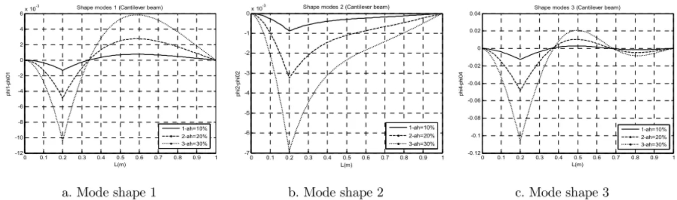
Figure 8: Change in first three mode shapes of cantilever FGM beam with a crack at 0.2m and depth varying from a/h=10% to 30%.
0 0.1 0.2 0.3 0.4 0.5 0.6 0.7 0.8 0.9 1 -0.06
-0.05 -0.04 -0.03 -0.02 -0.01 0 0.01
0.02 Shape modes 1 (Simply supported beam)
ph
i1
-phi
01
L(m)
1-ah=10% 2-ah=20% 3-ah=30%
0 0.1 0.2 0.3 0.4 0.5 0.6 0.7 0.8 0.9 1 -0.1
-0.05 0 0.05 0.1
0.15 Shape modes 2 (Simply supported beam)
ph
i2
-phi
02
L(m)
1-ah=10% 2-ah=20% 3-ah=30%
0 0.1 0.2 0.3 0.4 0.5 0.6 0.7 0.8 0.9 1 -0.2
-0.15 -0.1 -0.05 0 0.05 0.1
0.15 Shape modes 3 (Simply supported beam)
ph
i4
-phi
04
L(m)
1-ah=10% 2-ah=20% 3-ah=30%
0 0.1 0.2 0.3 0.4 0.5 0.6 0.7 0.8 0.9 1 -14
-12 -10 -8 -6 -4 -2 0 2x 10
-3 Shape modes 1 (Beam with clamped ends)
ph
i1
-p
hi
01
L(m)
1-ah=10% 2-ah=20% 3-ah=30%
0 0.1 0.2 0.3 0.4 0.5 0.6 0.7 0.8 0.9 1 -0.1
-0.08 -0.06 -0.04 -0.02 0 0.02 0.04
0.06 Shape modes 2 (Beam with clamped ends)
ph
i2
-p
hi
02
L(m)
1-ah=10% 2-ah=20% 3-ah=30%
0 0.1 0.2 0.3 0.4 0.5 0.6 0.7 0.8 0.9 1 -0.15
-0.1 -0.05 0 0.05 0.1 0.15
0.2 Shape modes 3 (Beam with clamped ends)
ph
i3
-p
hi
03
L(m)
1-ah=10% 2-ah=20% 3-ah=30%
0 0.1 0.2 0.3 0.4 0.5 0.6 0.7 0.8 0.9 1 -12
-10 -8 -6 -4 -2 0 2 4 6x 10
-3 Shape modes 1 (Cantilever beam)
ph
i1
-phi
01
L(m)
1-ah=10% 2-ah=20% 3-ah=30%
0 0.1 0.2 0.3 0.4 0.5 0.6 0.7 0.8 0.9 1 -7
-6 -5 -4 -3 -2 -1 0x 10
-3 Shape modes 2 (Cantilever beam)
ph
i2
-phi
02
L(m)
1-ah=10% 2-ah=20% 3-ah=30%
0 0.1 0.2 0.3 0.4 0.5 0.6 0.7 0.8 0.9 1 -0.12
-0.1 -0.08 -0.06 -0.04 -0.02 0 0.02
0.04 Shape modes 3 (Cantilever beam)
ph
i4
-phi
04
L(m)
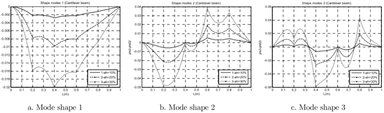
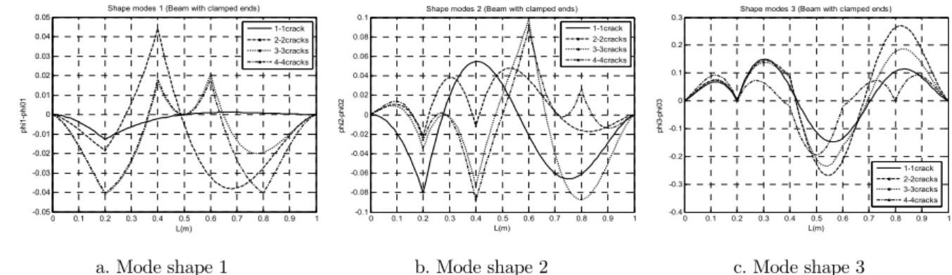
Deviation of the cracked mode shapes from the intact ones are computed for the beam with single crack at 0.2m (Figs. 6-8) and 4 equidistant cracks (Figs. 9-11) of various depth (10, 20, 30%) in different cases of boundary conditions. Natural frequencies corresponding to the mode shapes presented in the Figures are tabulated in Table 1. The deviations of mode shapes are computed also for the beam with various number of cracks (from 1 to 4) with the same depth 30% and shown in Figs. 12-14.
a. Mode shape 1 b. Mode shape 2 c. Mode shape 3
Figure 9: Change in first three mode shapes of simple support FGM beam with 4 equidistant cracks and depth a/h=10%, 20%, 30%.
a. Mode shape 1 b. Mode shape 2 c. Mode shape 3
Figure 10: Change in first three mode shapes of clamped end FGM beam with 4 equidistant cracks of the depth a/h=10%, 20%, 30%.
a. Mode shape 1 b. Mode shape 2 c. Mode shape 3
Figure 11: Change in first three mode shapes of cantilever FGM beam with 4 equidistant cracks of the depth a/h=10%, 20%, 30%.
0 0.1 0.2 0.3 0.4 0.5 0.6 0.7 0.8 0.9 1 -16
-14 -12 -10 -8 -6 -4 -2 0 2x 10
-3 Shape modes 1 (Simply supported beam)
ph
i1
-p
hi
01
L(m)
1-ah=10% 2-ah=20% 3-ah=30%
0 0.1 0.2 0.3 0.4 0.5 0.6 0.7 0.8 0.9 1 -0.04
-0.03 -0.02 -0.01 0 0.01 0.02 0.03
0.04 Shape modes 2 (Simply supported beam)
ph
i2
-p
hi
02
L(m)
1-ah=10% 2-ah=20% 3-ah=30%
0 0.1 0.2 0.3 0.4 0.5 0.6 0.7 0.8 0.9 1 -0.15
-0.1 -0.05 0 0.05
0.1 Shape modes 3 (Simply supported beam)
ph
i4
-p
hi
04
L(m)
1-ah=10% 2-ah=20% 3-ah=30%
0 0.1 0.2 0.3 0.4 0.5 0.6 0.7 0.8 0.9 1 -0.05
-0.04 -0.03 -0.02 -0.01 0 0.01
0.02 Shape modes 1 (Beam with clamped ends)
ph
i1
-p
hi
01
L(m)
1-ah=10% 2-ah=20% 3-ah=30%
0 0.1 0.2 0.3 0.4 0.5 0.6 0.7 0.8 0.9 1 -0.1
-0.08 -0.06 -0.04 -0.02 0 0.02 0.04 0.06 0.08
0.1 Shape modes 2 (Beam with clamped ends)
ph
i2
-p
hi
02
L(m)
1-ah=10% 2-ah=20% 3-ah=30%
0 0.1 0.2 0.3 0.4 0.5 0.6 0.7 0.8 0.9 1 -0.2
-0.15 -0.1 -0.05 0 0.05 0.1
0.15 Shape modes 3 (Beam with clamped ends)
ph
i3
-p
hi
03
L(m)
1-ah=10% 2-ah=20% 3-ah=30%
0 0.1 0.2 0.3 0.4 0.5 0.6 0.7 0.8 0.9 1 -0.02
-0.018 -0.016 -0.014 -0.012 -0.01 -0.008 -0.006 -0.004 -0.002
0 Shape modes 1 (Cantilever beam)
phi
1-ph
i01
L(m)
1-ah=10% 2-ah=20% 3-ah=30%
0 0.1 0.2 0.3 0.4 0.5 0.6 0.7 0.8 0.9 1 -0.05
-0.04 -0.03 -0.02 -0.01 0 0.01 0.02 0.03
0.04 Shape modes 2 (Cantilever beam)
ph
i2
-p
hi
02
L(m)
1-ah=10% 2-ah=20% 3-ah=30%
0 0.1 0.2 0.3 0.4 0.5 0.6 0.7 0.8 0.9 1 -0.06
-0.04 -0.02 0 0.02 0.04
0.06 Shape modes 3 (Cantilever beam)
ph
i3
-p
hi
03
L(m)
a. Mode shape 1 b. Mode shape 2 c. Mode shape 3
Figure 12: Change in first three mode shapes of simple support FGM beam with various number of cracks (from 1 to 4) and depth a/h=30%.
a. Mode shape 1 b. Mode shape 2 c. Mode shape 3
Figure 13: Change in first three mode shapes of clamped end FGM beam with various number of cracks (from 1 to 4) and depth a/h=30%.
a. Mode shape 1 b. Mode shape 2 c. Mode shape 3
Figure 14: Change in first three mode shapes of cantilever FGM beam with various number of cracks (from 1 to 4) and depth a/h=30%.
0 0.1 0.2 0.3 0.4 0.5 0.6 0.7 0.8 0.9 1 -0.06
-0.04 -0.02 0 0.02 0.04
0.06 Shape modes 1 (Simply supported beam)
ph
i1
-phi
01
L(m)
1-1crack 2-2cracks 3-3cracks 4-4cracks
0 0.1 0.2 0.3 0.4 0.5 0.6 0.7 0.8 0.9 1 -0.2
-0.15 -0.1 -0.05 0 0.05 0.1
0.15 Shape modes 2 (Simply supported beam)
ph
i2
-phi
02
L(m)
1-1crack 2-2cracks 3-3cracks 4-4cracks
0 0.1 0.2 0.3 0.4 0.5 0.6 0.7 0.8 0.9 1 -0.25
-0.2 -0.15 -0.1 -0.05 0 0.05 0.1 0.15
0.2 Shape modes 3 (Simply supported beam)
ph
i4-phi
04
L(m) 1-1crack
2-2cracks 3-3cracks 4-4cracks
0 0.1 0.2 0.3 0.4 0.5 0.6 0.7 0.8 0.9 1 -0.05
-0.04 -0.03 -0.02 -0.01 0 0.01 0.02 0.03 0.04
0.05 Shape modes 1 (Beam with clamped ends)
phi
1-ph
i01
L(m)
1-1crack 2-2cracks 3-3cracks 4-4cracks
0 0.1 0.2 0.3 0.4 0.5 0.6 0.7 0.8 0.9 1 -0.1
-0.08 -0.06 -0.04 -0.02 0 0.02 0.04 0.06 0.08
0.1 Shape modes 2 (Beam with clamped ends)
ph
i2
-p
hi
02
L(m)
1-1crack 2-2cracks 3-3cracks 4-4cracks
0 0.1 0.2 0.3 0.4 0.5 0.6 0.7 0.8 0.9 1 -0.4
-0.3 -0.2 -0.1 0 0.1 0.2
0.3 Shape modes 3 (Beam with clamped ends)
ph
i3
-p
hi
03
L(m)
1-1crack 2-2cracks 3-3cracks 4-4cracks
0 0.1 0.2 0.3 0.4 0.5 0.6 0.7 0.8 0.9 1 -0.02
-0.015 -0.01 -0.005 0 0.005
0.01 Shape modes 1 (Cantilever beam)
ph
i1
-phi
01
L(m) 1-1crack
2-2cracks 3-3cracks 4-4cracks
0 0.1 0.2 0.3 0.4 0.5 0.6 0.7 0.8 0.9 1 -0.06
-0.04 -0.02 0 0.02 0.04 0.06 0.08
0.1 Shape modes 2 (Cantilever beam)
ph
i2
-phi
02
L(m)
1-1crack 2-2cracks 3-3cracks 4-4cracks
0 0.1 0.2 0.3 0.4 0.5 0.6 0.7 0.8 0.9 1 -0.2
-0.15 -0.1 -0.05 0 0.05 0.1
0.15 Shape modes 3 (Cantilever beam)
ph
i3
-phi
03
L(m)
Observing graphs in the Figures allows one to make some remarks as follows:
a) Deviation of mode shapes is typically non-smooth (sharp peak) at crack positions, so that crack location could be easily discriminated by using the wavelet analysis of mode shapes.
b) Height of the sharp peaks in the graphs of mode shape deviation is monotonically increasing with crack depth. This enables to estimate also crack depth by the wavelet coefficient of mode shape at the crack location;
c) Effect of symmetric cracks on the mode shape is the same for beam with symmetric boundary conditions and symmetric cracks make no change in mode shape at the beam middle.
d) There are some positions on beam that presence of crack at these points makes no change in a mode shape. Such the points on beam are called invariable for the mode shape. For instance, midpoint of simply supported beam (x=0.5m) is invariable point for the fundamental mode shape (Fig.6a) or x=0.356m and x=0.67m – are invariable for the third mode shape of cantilever beam (Fig.8c).
All the mentioned notices are useful indication for crack detection in FGM beam by measurements of mode shapes.
4 CONCLUSIONS
In this paper, the consistent theory of free vibration of multiple cracked FGM Timoshenko beam is formulated on the base of the power law distribution of FGM material, rotation spring model of crack and actual position of neutral axis.
The obtained frequency equation and mode shape of cracked FGM Timoshenko beam provide a simple approach to study not only free vibration of the beam but also the inverse problem of material and crack identification in FGM structures.
Numerical analysis demonatrates that mode shapes of FGM Timoshenko beam are sufficiently sensitive to cracks and dependent on material properties and geometric parameter of the beam.
References
A. Banerjee, B. Panigrahi, G. Pohit (2015), “Crack modelling and detection in Timoshenko FGM beam under trans-verse vibration using frequency contour and response surface model with GA”, Nondestructive Testing and Evaluation; DOI.10.1080/10589759.2015.1071812.
D. Wei, Y.H. Liu, Z.H. Xiang (2012), “An analytical method for free vibration analysis of functionally graded beams with edge cracks”, Journal of Sound and Vibration, 331, 1685-1700.
F. Erdogan, B.H. Wu (1997), “The surface crack problem for a plate with functionally graded properties”, Journal of Applied Mechanics, 64, 448-456.
H. Su, J.R. Banerjee (2015), “Development of dynamic stiffness method for free vibration of functionally graded Timo-shenko beam”, Computers & Structures, 147, 107-116.
J. Yang, Y. Chen (2008), “Free vibration and buckling analyses of functionally graded beams with edge cracks”, Com-posite Structure, 83, 48-60.
J. Yang, Y. Chen, Y. Xiang, X.L. Jia (2008), “Free and forced vibration of cracked inhomogeneous beams under an axial force and a moving load”, Journal of Sound and Vibration, 312, 166–181.
K. Sherafatnia, G.H. Farrahi, S.A. Faghidian (2014), “Analytic approach to free vibration and bucking analysis of functionally graded beams with edge cracks using four engineering beam theories”, International Journal of Engieering, 27(6), 979-990.
L.L. Ke, J. Yang, S. Kitipornchai, Y. Xiang (2009), “Flexural vibration and elastic buckling of a cracked Timoshenko beam made of functionally graded materials”, Mechanics of Advanced Materials and Structures, 16, 488–502.
M.A. Eltaher, A.E. Alshorbagy, F.F. Mahmoud (2013), “Determination of neutral axis position and its effect on natural frequencies of functionally graded macro/nanobeams”, Composite Structures, 99: 193-201.
N. Wattanasakulpong, V. Ungbhakorn (2012), “Free Vibration Analysis of Functionally Graded Beams with General Elastically End Constraints by DTM”, World Journal of Mechanics, 2, 297-310
N.N. Huyen and N.T. Khiem (2016), “Uncoupled vibration in functionally graded Timoshenko beam”, VAST Journal of Science and Technology, 54(6) 785-796. DOI: 10.15625/0866-708X/54/6/7719.
N.T. Khiem and N.N. Huyen (2016), “A method for crack identification in functionally graded Timoshenko beam”, Nondestructive Testing and Evaluation. FirstOnline Oct. 2016. DOI:10.1080/10589759.2016.1226304.
N.T. Khiem, N.D. Kien, N.N. Huyen (2014), “Vibration theory of FGM beam in the frequency domain”, Proceedings of National Conference on Engineering Mechanics celebrating 35th Anniversary of the Institute of Mechanics, VAST, April 9, 93-98 (in Vietnamese).
N.T. Khiem, T.V. Lien (2002), “The dynamic stiffness matrix method in forced vibration analysis of multiple cracked beam”, Journal of Sound and Vibration, 254(3), 541-555.
S. Kitipornchai, L.L. Ke, J. Yang, Y. Xiang (2009), “Nonlinear vibration of edge cracked functionally graded Timo-shenko beams”, Journal of Sound and Vibration, 324, 962-982.
S.D. Akbas (2013), “Free Vibration Characteristics of Edge Cracked Functionally Graded Beams by Using Finite Element Method”, International Journal of Engineering Trends and Technology, 4(10).
T. Yan, S. Kitipornchai, J. Yang, X.Q. He (2011), “Dynamic behavior of edge-cracked shear deformable functionally graded beams on an elastic foundation under a moving load”, Composite Structures, 93, 2992-3001.
T.V. Lien, N.T. Duc and N.T. Khiem (2016), “Free vibration analysis of functionally graded Timoshenko beam using dynamic stiffness method”, Journal of Science and Technology in Civil Engineering, National University of Civil Engi-neering, 31, 19-28.
Tran Van Lien, Trinh Anh Hao (2013), “Determination of the mode shapes of a multiple cracked beam element and its application for the free vibration analysis of a multi-span continuous beam”, Vietnam Journal of Mechanics, Vietnam Academy of Science and Technology, 35(4), 313-323.
Z.G. Yu, F.L. Chu (2009), “Identification of crack in functionally graded material beams using the p-version of finite element method”, Journal of Sound and Vibration, 325 (1–2), 69–84.
APPENDIX
A1. Constants in formula (4)
,
,
(
)
,1
,
.
;
)
(
;
,
,1
)
(
,
,
2 0 0
22 12 11
33 2
0 0
22 12 11
A
A A
dA
h
z
h
z
z
I
I
I
dA
z
G
A
dA
h
z
h
z
z
E
A
A
A
2 3 22 2 12 11 33 2 3 22 0 2 12 111
2
2
)
3
(
3
3
;
1
)
2
(
2
2
1
;
1
;
1
2
2
)
3
(
3
3
2
1
;
1
)
2
(
2
2
;
1
n
n
n
n
n
n
bh
I
n
n
n
n
bh
I
n
n
bh
I
n
nG
G
bh
A
n
nE
E
n
nE
E
n
nE
E
bh
A
h
h
n
nE
E
n
nE
E
bh
A
n
nE
E
bh
A
b t b t b t b t b t b t b t b t b t b t b t b t b tA2. General solution of cub algebraic equation
0
2
3
a
b
c
where
22 11 2 11 22 11 2 12 22 11 33 11 2 4 22 11 2 22 11 11 22 22 11 33 11 22 11 2 12 22 11 4 22 11 11 22 22 11 33 11 2;
A
A
I
A
A
I
I
I
A
I
c
A
I
A
A
A
I
A
I
A
I
A
A
I
I
I
b
A
A
A
I
A
I
A
I
a
Roots of cub algebraic equation are
1(
),
2(
),
3(
)
2
/
)
/
(
3
2
/
)
/
(
3
/
;
/
3
/
1 2,3 1 11
a
u
b
u
a
u
b
u
i
u
b
u
where 1 3 1 2 1 1 3 / 1 3 2 1 3 11
/
27
)
;
/
6
/
2
;
/
3
/
9
;
/
27
(
a
b
c
a
a
ab
c
b
b
a
c
a
a
u
A3. Differential matrix operators
Simply supported (S):
u
(
x
,
t
)
M
(
x
,
t
)
w
(
x
,
t
)
0
1
0
0
0
0
0
1
2212 x x
S
A
A
B
Pined (P):
N
(
x
,
t
)
M
(
x
,
t
)
w
(
x
,
t
)
0
1
0
0
0
0
22 12 12 11 x x x xP