Angelo Passaro Instituto de Estudos Avançados São José dos Campos – Brazil [email protected]
Dermeval Carinhana Jr* Instituto de Estudos Avançados
São José dos Campos – Brazil [email protected]
Enizete Aparecida Gonçalves Instituto Nacional de Pesquisas Espaciais São José dos Campos – Brazil [email protected]
Marcio Moreira da Silva Instituto de Estudos Avançados
São José dos Campos – Brazil [email protected]
Ana Paula Lasmar Guimarães Universidade Estadual Paulista Guaratinguetá – Brazil [email protected]
Nancy Mieko Abe Instituto de Estudos Avançados
São José dos Campos – Brazil [email protected]
Alberto Monteiro dos Santos Instituto de Estudos Avançados São José dos Campos – Brazil [email protected]
*author for correspondence
The use of molecular spectra
simulation for diagnostics of
reactive lows
Abstract: The C2* radical is used as a system probe tool to the reactive
low diagnostic, and it was chosen due to its large occurrence in plasma and combustion in aeronautics and aerospace applications. The rotational temperatures of C2* species were determined by the comparison between
experimental and theoretical data. The simulation code was developed by the authors, using C++ language and the object oriented paradigm, and it includes a set of new tools that increase the eficacy of the C2
* probe to
determine the rotational temperature of the system. A brute force approach for the determination of spectral parameters was adopted in this version of the computer code. The statistical parameter c2 was used as an objective
criterion to determine the better match of experimental and synthesized spectra. The results showed that the program works even with low-quality experimental data, typically collected from in situ airborne compact apparatus. The technique was applied to lames of a Bunsen burner, and the rotational temperature of ca. 2100 K was calculated.
Keywords: Optical emission spectra, Computerized simulation, Combustion control, Computer programs, Rotational spectra.
INTRODUCTION
Combustion processes and plasma formation are inherent phenomena of the aerospace technology. Operation of propulsion artifacts, like gas turbine and rocket engine, and shock-wave formation, as observed in hypersonic
light and re-entrance procedures, are the most common
examples of this association. In general, both systems constitute a high-temperature environment, with electrons and ionized species produced by a complex chemistry
and a time-varying turbulent low ield (Zel’dovich and
Raizer, 2002). The measurement of any basic system data, such as temperature and concentration of major species
and intermediated radicals and low velocities, requires the employment of speciic diagnostic techniques.
For some kinds of combustion systems, which includes aeronautic and aerospace applications, the use of conventional probes, such as thermocouples and gas analyzers, for combustion diagnostic is not possible or can cause structural
problem and aerodynamic instability, disturbing the system
(Gregory, 2005). In these cases, the reliability of measurements is affected by the high-temperature observed in these lames and by perturbations in the low stability caused by probe
insertion. As alternative, these systems can be monitored by using nonintrusive methods, especially those based on optical properties, i.e., in the absorption or emission of radiation of the
system (Docquier and Candel, 2002). Among them, the natural
or spontaneous emission spectroscopy of radical species shows some remarkable advantages, as it only needs a simple, low-cost, and compact experimental apparatus. These features point to the use of the emission spectroscopy as an important and powerful tool to support active control of combustion processes, where a real time and in situ system monitoring is
required (Ballester and Garcia-Armingol, 2010).
Emission of lames is due to chemical reactions that produce
intermediate chemical species, like, for example, free radicals in excited states. The radiation emission of these radicals is known as chemiluminescence. In hydrocarbon
fuel lames, the most intense emissions are associated with
C2*, CH* e OH* species (Durie, 1952; Kane and Broida,
1953). The asterisk denotes the electronic state associated Received: 26/11/10
Accepted: 01/02/11
with each molecule. Apart from spectroscopic constants and experimental factors, the intensity of radical emission spectra is related to the system temperature. This relation is
expressed by the Boltzmann´s equation, which is given by:
theoretical calculation, which can generate nondesirable artifacts, as spectral line losses.
The aim of this paper is to present molecular spectra simulation as a combustion and plasma diagnostic tool. The species chosen as probe for rotational temperature
determination was the C2* excited radical. This
intermediated reaction product is largely present in all combustion processes containing fossil fuel. It is also present in plasmas formed by high-temperature exposure and ion irradiation of carbonic composites, which are
materials with several aerospace applications (Arepalli et al., 2000; Paulmier et al., 2001).
SPECTRA SIMULATION
The computer code for spectra simulation used in this paper was developed by the authors using the C++ language and the object oriented paradigm, and it follows the procedure
presented in Pellerin et al. (1996) and Acquaviva (2004)
to synthesize the spectra. The computer code allows the visualization of the experimental spectra and of the theoretical one, of the computed emission lines, of both wavelength and intensity, and of the relative contribution
of branches P, Q, and R for each C2* band. The comparison
of theoretical and experimental spectra can be done by visual inspection, with both spectra superposed in one graph and showing the discrepancy between them for each wavelength in a second plot.
The theoretical spectrum curves are obtained following
the steps: (i) calculation of the spectral lines position; (ii) determination of its relative intensities and inally (iii) application of a Gaussian-type broadening factor. The irst
step is carried out using spectroscopic data taken from
literature (Pellerin et al., 1996). The two latter steps are
dependent of the rotational temperature and total spectral resolution, respectively.
The spectra simulator allows the computation of a single spectrum from the temperature and resolution, and the solution of the inverse problem, determining an optimum
pair (temperature, resolution) that minimizes differences
between the simulated and experimental spectra. A brute force approach is adopted in this version of the computer
code. A range for these two parameters is deined by the
user, as well as the variation step of each of them. The implementation explores the multicore characteristic of the modern processors in order to determine both temperature and resolution in a very short time.
The number of computer cores is detected automatically by
the computer program and an adequate number of threads
is launched, parallelizing coarse grain computations. From these data, synthesized spectra for each pair combination,
(1)
-=
-kT E CS
I JJ 4 J'
"
'
Ȝ
exp( )
where SJ´J” is the line strength of a transition from the upper
(J´) to the lower (J”) rotational state of the excited species; EJ´
is the rotational energy of the upper rovibrational level; C is a proportionality constant related to experimental factors, like detector and diffraction grating responses, which attenuate
or maximize the emission signal; is the line wavelength
associated with the transition; and k is the Boltzmann factor (Herzberg, 1950). Thus, the challenge of combustion diagnosis
is to establish a consistent relation between microscopic features of the system, spontaneous emission of chemical species generated by fuel burning, and macroscopic property, e.g., its kinetics temperature, which is the most common
temperature concept adopted to characterize a lame.
Considering that the emission spectrum follows the
Boltzmann distribution given by Eq. 1, a plot of the natural
logarithm of line intensities versus the energy term shows
a straight line whose slope is the inverse of the rotational temperature. In some cases, the rotational temperature of the intermediate species of hot gases is very close to the kinetic temperature, because the translational and
rotational energies of a molecule equilibrate within a
trajectory of a few mean free path length by collisional
processes with other species (Lapworth, 1974). In nonequilibrium systems, as in hypersonic lows (Fujita et al., 2002; Ivanov et al., 2008; Tsuboi; Matsumoto, 2006), supersonic combustion (Do et al., 2008), or plasmas generated by spacecraft during reentry (Blackwell et al., 1997), the various forms of energy are not in equilibrium,
and there is not one temperature value able to describe all
physical chemistry processes in course (Reif et al., 1973).
In these cases, rotational temperature is useful to provide information about chemical reactivity of the medium and
produced thermal energy (Acquaviva, 2004).
A direct and simple method to determine the rotational temperature is the comparison of experimental spectra with a synthetic one. The latter can be computed by
applying Eq. 1 to each rotational transition belonging to a speciic natural emission band. The inal spectrum proile
is synthesized by the convolution of every spectral line
using, for example, a Gaussian-type function. Most of the
temperature/resolution, is iteratively computed. Basically, each set of input data in the ranges deined by the user is used to
simulate a spectrum. Every synthesized spectrum is compared with the experimental one to choose the synthesized spectrum
that better matches the experimental one. The quality of each synthesized spectrum is deined by comparison with the experimental one, using the chi-squared statistical parameter (2) as a igure of merit. The computer code adopts the full wavelength range as default, but this can be a bad choice if several bands are under consideration or if the contribution of other radicals is important in the experimental spectrum. The
user can deine a particular range of wavelength, for instance,
a region where only a given band of a molecule contributes
appreciably to the spectra, as basis for the chi-squared computation in order to reduce the inluence of these factors
and improve the parameter determination.
These tools are fundamental to reduce the error usually associated in literature with the determination of temperature. Although a detailed description of the tools implemented in our computer code is out of the scope of this work, some few special characteristics are presented when needed in the Results section.
SPECTRA ACQUISITION
Bunsen-type lames were investigated to illustrate
employment and capability of the theoretical simulation to obtain the temperature related to the experimental spectra.
The fuel burned was liqueied petroleum gas (LPG). The optical system consisted on a TRIAX 550 (Jobin Yvon) monochromator of 0.5 m focal length (f), equipped with a
1.200 lines.mm-1 diffraction grating, with blaze at 500 nm.
The instrumental resolutions (inst) resulting were 0.061,
0.095, and 0.13 nm, for exit slit apertures of 30, 60 and 90 µm, respectively. These values were calculated from
the measurement of the full width at half maximum
(FWHM) of the emission line at 546 nm of a low-pressure
discharge Hg lamp. Three C2* spectra were acquired in the same experimental conditions for each instrumental
resolution. Flame radiation was collected by a iber optic
bundle connected to the spectrometer light entrance.
Emission signal was detected by a Hamamatsu R928P phototube, with 950 V as work voltage. Spectra were obtained in the 502 to 518 nm range, which corresponds
to the d3Π g → a
3Π
u electronic transition, known as Swan
band (Gaydon, 1957). All spectra were measured at the region corresponding to the end of the inner lame cone.
RESULTS AND DISCUSSION
Typical experimental C2* emission spectra acquired with
three instrumental resolutions, 0.061, 0.096 and 0.13 nm
are presented in Fig. 1. These resolutions are easily obtained
with commercial, low-cost, and compact spectrometers. These characteristics present special importance regarding
the acquisition of data from aeronautics and aerospace
applications. In most cases, the payload weight is a critical limiting variable, and the use of compact spectrometers of
low-resolution is an interesting choice for in situ airborne
diagnostic of plasma or combustion (Gord and Fiechtner, 2001; Knight et al., 2000).
Figure 1: Emission spectrum of the Swan band of the C2* radical. Measured instrumental resolution were: (a) 0.061 nm, (b) 0.095 nm and (c) 0.13 nm.
510 511 512 513 514 515 516 517 0.0
0.2 0.4 0.6 0.8 1.0
I (a.u.)
(nm) (a)
1-1 band
0-0 band
Ȝ
510 511 512 513 514 515 516 517 0.0
0.2 0.4 0.6 0.8 1.0
(b)
I (u.a.)
(nm)
1-1 band
0-0 band
Ȝ
510 511 512 513 514 515 516 517 0.0
0.2 0.4 0.6 0.8 1.0
1-1 band (c)
I (u.a.)
(nm)
0-0 band
The spectra were normalized with respect to the band-head of the 0-0 vibrational band. The use of different instrumental resolutions provides spectra with remarkable differences. Characteristic intense peaks are observed at ca.
516.6 and 513.0 nm, corresponding to the band-heads of
0-0 and 1-1 vibrational bands, respectively. In the present
paper, only the peaks of 0-0 band between 513.5 -516 nm
were used in the determination of temperature. This range
contains an appreciable quantity of “thermometric peaks”,
i.e., peaks whose relative intensities are more sensitive to
changes in the rotational temperature (Carinhana, 2006). However, the degradation of spectrum proiles caused by
peak broadening is stronger in this region.
In the following subsections, we illustrate the use of the simulation tool to aid the temperature determination for
the case of higher resolution spectra (0.061 nm).
A - Procedure for the rotational temperature determination
The irst issue for temperature determination is the choice of initial values of the rotational temperature (Trot) and of
the spectral resolution (spec), which will be used as input data for computing the theoretical spectra. The initial input
data were set as Trot = 1850 K and inst = 0.061 nm. The
chosen temperature corresponds to the temperature for
Bunsen-type lames at the investigated region, determined by McPherson and Henderson (1927). The initial value of spectral resolution was assumed to be equal to the
instrumental resolution determined with the Hg lamp.
Figure 2 shows the experimental spectrum overlapped with the synthesized one. It can be noticed differences in the wavelength of corresponding peaks in the experimental and synthesized spectra. These differences can be explained by small deviations in spectral calibration of the experimental apparatus.
One of the tools implemented in the simulator allows a wavelength adjustment in order to match both experimental
and synthesized spectra in a region between two deined
peaks. This process is done to correct these deviations, improving the procedure taken in the next step to determine the temperature. To carry out the matching, the correspondence of two known pair of peaks of
experimental and theoretical spectra, deined by the user, is set in a speciic graphic window. In this example, a
match was accomplished choosing as reference peaks the band-head of the 0-0 and 1-1 bands, that is, the limits
of the region of interest regarding the 0-0 band (Fig. 3).
Apparently, a reasonable match between both spectra is shown. Nevertheless, some remarkable differences in the peak intensities can be observed.
The next step is the optimized values determination of the simulation parameters. In fact, as previously explained, a brute force approach is used to solve an inverse problem. For that, a range of Trot and of , and the number of steps
for each of them, is deined by the user. The program computes a sequence of spectra for each (Trot, spec) pair,
and also calculates the respective value of 2 comparing
the synthesized spectra with the experimental one. These results are expressed graphically as a family of curves of 2 versus T
rot for each value of spec. The optimized parameters of the theoretical spectrum are given by the
Figure 2: Experimental spectrum with instrumental resolution of 0.061 nm superimposed to a synthesized spectrum computed with rotational temperature of 1850 K and spectral resolution of 0.061 nm.
512.5 1e+003
800
600
400
200
0
513.5 514.5 515.5 516.5 517.5
Intensity (A.U.)
Wavelength
Figure 3: Experimental spectrum with instrumental resolution of 0.061 nm superimposed to a synthesized spectrum computed with rotational temperature of 1850 K and spectral resolution of 0.061 nm after the matching operation.
1e+003
800
600
400
200
0
Intensity (A.U.)
512.5 513.5 514.5 515.5 516.5 517.5
Wavelength (nm)
inst (nm) Trot (K) spec (nm)
0.061 2113 (77) 0.069(2)
0.095 2173 (34) 0.0961(16)
0.13 2616 (77) 0.1451(31)
best spectra match, i.e., by the point where the minimum value of 2 is observed. Examples of these calculated
curves are shown in Figs. 4 and 5.
With respect to Fig. 4, the testing range of Dl was arbitrarily assigned as 0.061 ± 0.01 nm, i.e., ca. 15% for
lower and upper values. A similar criterion was adopted
for the Trot range, which was chosen as 1,850 ± 270 K. The
number of steps for both ranges was 32. Of course, these were not good choices because it is not certain that the family of curves have reached a minimum. The optimized temperature can be out of the chosen range.
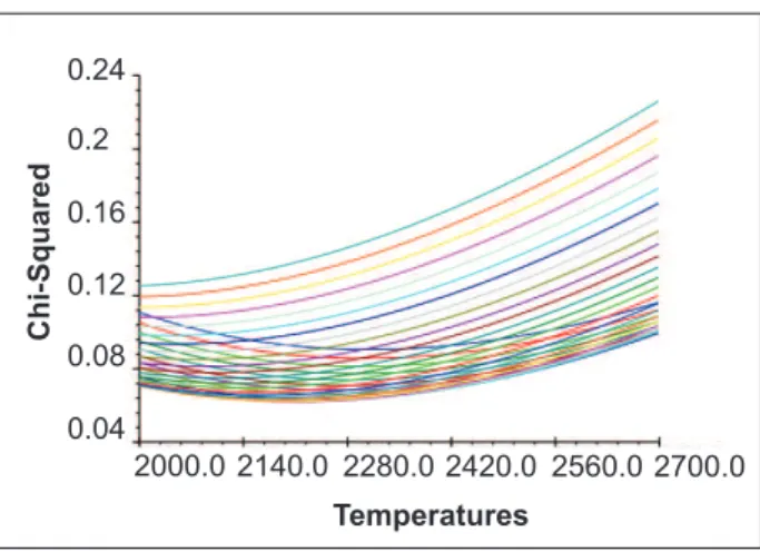
Figure 5 shows a new set of curves obtained for 2000 ≤ Trot ≤ 2,700 K and 0.061 ≤ spec ≤ 0.081 nm. From
this family of curves, the minimum of c2 corresponds to
the pair Trot = 2113 K and spec = 0.069 nm. Note that
the determined rotational temperature was considerably higher than the original input data.
The same procedure was applied to determine the temperature associated with the other experimental spectra. Values of Trot and spec presented in Table 1 correspond to
the mean values computed from the set of spectra acquired
for each instrumental resolution. The errors, presented inside the parenthesis, correspond to the standard deviation.
Figure 6 shows the spectrum synthesized with the
parameters presented in Table 1 for inst 0.061 nm
superposed to one of the experimental spectra. Figure
7 shows the deviation between the same experimental
spectrum and the synthesized spectra referring to Figs. 2, 3, and 6. The deviation graph is other of the tools implemented in the computational program, and it is very useful in the superposing spectra evaluation. The optimum synthesized spectrum is in very good agreement with the experimental one. Only small differences are observed in
the region between 513.2 and 516 nm, distributed around
zero, i.e., in the region of the thermometric peaks.
Here, it is important to say that instrumental resolution
(inst) is not the unique contribution to the peak proile
of the emission spectra. There are physical-chemistry
phenomena, like Doppler Effect and collisional processes
involving the chemical species present in the system, which also cause line broadening of the spectrum
(Gaydon, 1957; Griem, 1997). As both factors are mainly
dependent on the temperature and pressure of the system, respectively, it can be accepted that they are negligible
Spectrum 1 Spectrum 2 Spectrum 3
Trot (K) 2555 2592 2814
spec (nm) 0.146 0.141 0.146
Table 2: Trot and spec calculated from experimental spectra with nominal resolution of 0.13 nm (lower resolution)
Figure 4: 2 versus T
rot curves used in optimization procedure of spectral parameters. Each one corresponds to a value of spec between 0.05 and 0.07 nm. The minimum value of 2 corresponds to the pair T
rot = 2120 K and
spec = 0.07 nm.
0.4
0.313
0.225
0.138
0.05
1550.0 1700.0 1850.0 200.0 2150.0
Temperatures
Chi-Squared
Figure 5: Final 2 versus T
rot curves used in optimization procedure of spectral parameters. The minimum value of 2 corresponds to the pair T
rot = 2,113 K and
spec = 0.069 nm.
0.24
0.2
0.16
0.12
0.08
0.04
2000.0 2140.0 2280.0 2420.0 2560.0 2700.0
Temperatures
Chi-Squared
Figure 6: Final synthesized spectrum overlapped with an experimental one. Trot = 2,113 K and
spec = 0.069 nm.
0.04
512.0 513.0 514.0 515.0 516.0 517.0
Wavelength (nm)
Intensity (A.U.)
800
600
400
200
0 1e+003
for low-pressure Hg lamp, and that inst is given by the
broadening show appreciable inluence. Thus, the spectral
resolution of C2* emission spectra is expected to be larger
than the inst.
In all cases, the results regarding spec were consistent with the expected behavior: all of them were higher than
the inst. The temperature obtained from the spectra
with nominal resolution of 0.061 and 0.095 nm agrees,
considering the standard deviation.
The difference observed in temperature between the
computed and the original input data (1850 K) is not related
to the computer code response, but to the deactivation processes of the C2* radical. In fact, C
2
* radical rotational
temperatures have been described in literature as being
higher than the theoretical equilibrium lame temperature (Gaydon and Wolfhard, 1970). This means that the rotational degrees of freedom are not in equilibrium and Boltzmann-Maxwell distribution of velocities is not
strictly followed. The average number of collisions in
the excited state is not suficient to establish a rotational distribution equivalent to the temperature associated with
the translational, or kinetic, mode. The emission spectra, therefore, correspond to a description of the rotationally excited states of the C2* species. This feature of C
2
* radical
is useful to describe the physical chemistry processes
of reactive lows with the presence of organic reactants (Rond et al., 2007). In these systems, the nonequilibrium
situation produces a strong radiative emission from the excited species, and this radical can be used as a probe to indicate the temporal evolution of rotational temperature.
B - Limits of the proposed approach
As already stated, the temperature determination by spectra simulation is based on the comparison of experimental
and computed spectra proiles. The analyzed range of wavelengths has to contain an appreciable quantity of
peaks, whose relative intensities are more sensitive to changes in the rotational temperature. As the resolution
decreases (greater values of spec), a degradation of
spectrum proiles caused by peak broadening is expected,
reducing the elements for the pair determination
(Trot, spec). In this case, the determination of the temperature can be a problem.
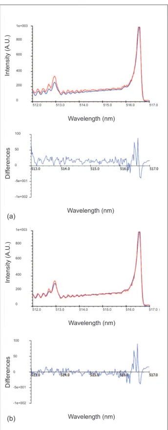
Spectra with 0.13 nm instrumental resolution are examples of cases where the spectra broadening results in a lack
of thermometric peaks (Fig. 8b). Table 1 shows that the rotational temperature obtained for the spectra acquired
with inst = 0.13 nm is much higher than the value presented in other cases. The computer code was able to
reproduce consistently the temperature and spec even for
this set of experimental spectra, resulting in a rotational
temperature above 2,600 K with a standard deviation of
the same magnitude as the other cases.
A simple procedure was performed to test the former result consistency: the experimental spectra were compared with the
simulated ones with Trot of 2,150 K as input data. This value
corresponds to the average Trot presented in Table 1 computed
from the other two more resolved spectra. The superposed
spectra in Figs. 8a and 8b suggest that the experimental one
with larger nominal resolution do not present the same Trot of
Figure 7: Deviation between synthesized spectrum and the experimental one: (a) original data – 1,850 K; (b) after spectra matching - 1,850 K; and (c) optimized spectrum – 2,113 K. Note that the amplitude of the deviation between the spectra decreases systematically from (a) to (c).
Wavelength (nm)
Wavelength (nm)
Wavelength (nm)
Dif
ferences
Dif
ferences
Dif
ferences
400
300 200
100
0 -1e+002
-2e+002
100
50
0
-1e+002 -5e+001
100
50
0
-1e+002 -5e+001
(a)
(b)
the others, because the synthesized spectrum is systematically
below the experimental in the region of interest, from 513.2 to 517 nm. The temperature determined for each spectrum, in
this case, is presented in Table 2, which can indicate that the
mixture of oxygen and LPG was not anymore stable when these spectra were acquired.
Additional tests have to be carried out in order to determine the actual limitations of the proposed approach.
CONCLUSIONS
The use of C2* molecular emission spectroscopy allied
with spectra simulation for reactive lows diagnostic
was presented. The presented methodology was able to
determine consistently the temperature for C2* spectra
acquired within a large range of spectral resolution, including low-quality spectrum data. The developed computational program allows a quick determination
of the C2* rotational temperature associated with the
0-0 band. A brute force approach to solve the inverse
problem, allied to a C2* spectra simulator, which explores
the multicore capability of the modern computers, proved to be a good strategy for determining the optimum pair
(Trot, spec). The time frame to obtain the optimum pair
is compatible with the spectrum acquisition time, making this one useful tool to lame diagnostics in laboratory.
This has remarkable importance for aeronautics and aerospace applications, where the use of light and compact spectrometers of low-resolution can reduce the payload weight. The computed values of C2* rotational temperatures, considering the higher
resolution spectra,were ca. 2150 K for a Bunsen burner lame.
This value is ca. 6% higher than the one reported in literature, which indicates, as expected, that the Bunsen-type lames are not completely in equilibrium state.
Nowadays, the computer code computes up to ive Swan
bands, but the determination of the rotational temperature is based only on the thermometric peaks of the 0-0 band. New tools to explore the additional bands are under development.
ACKNOWLEDGMENTS
Angelo Passaro wishes to thank the inancial support of the Brazilian National Council for Research and Development (CNPq), under grant: 310768/2009-8.
REFERENCES
Acquaviva, S., 2004, “Simulation of Emission Molecular
Spectra by a Semi-Automatic Programme Package:
The Case of C-2 and CN Diatomic Molecules Emitting During Laser Ablation of a Graphite Target in Nitrogen
Environment”, Spectrochimica Acta Part a-Molecular and Biomolecular Spectroscopy, Vol. 60, No. 8-9, pp. 2079-2086. doi:10.1016/j.saa.2003.10.040
Figure 8: Comparison of synthesized and experimental spectra for two different set of input parameters : (a)
Trot = 2,150 K and (b) Trot = 2,616 K. The same
= 0.145 nm is used in both cases.
Wavelength (nm)
Wavelength (nm)
Intensity (A.U.)
Dif
ferences
1e+003
800
600
400
200
0
100
50
0
-1e+002 -5e+001
Wavelength (nm)
Dif
ferences
100
50
0
-1e+002 -5e+001
512.0 513.0 514.0 515.0 516.0 517.0
Wavelength (nm)
Intensity (A.U.)
1e+003
800
600
400
200
0
512.0 513.0 514.0 515.0 516.0 517.0 (a)
(b)
Arepalli, S., Nikolaev, P., Holmes, W. and Scott, C. D., 2000, “Diagnostics of Laser-Produced Plume under Carbon Nanotube Growth Conditions”, Applied Physics A-Materials Science & Processing, Vol. 70, No. 2, pp. 125-133. doi: 10.1007/s003390050024
Ballester, J., García-Armingol, T., 2010, “Diagnostic Techniques for the Monitoring and Control of Practical Flames”, Progress in Energy and Combustion Science, Vol. 36, No. 4, pp. 375-411. doi: 10.1016/j. pecs.2009.11.005
Blackwell, H. E.; Scott, C.D.; Arepalli, S., 1997, “Measured Nonequilibrium Temperatures in a Blunt Body Shock Layer in Arc Jet Nitrogen Flow”, 32nd Thermophysics
Conference, AIAA.
Carinhana Junior, D., 2006, “Determination of Flame Temperature by Emission Spectroscopy” (In Portuguese), Ph.D. Thesis, State University of Campinas, Campinas, SP, Brazil, 129p.
Do, H., Mungal, M. G. and Cappelli, M. A., 2008, “Jet Flame Ignition in a Supersonic Crosslow Using a Pulsed Nonequilibrium Plasma Discharge”, IEEE Transactions on Plasma Science, Vol. 36, No. 6, pp. 2918-2923.
Docquier, N., Candel. S., 2002, “Combustion Control and Sensors: A Review”, Progress in Energy and Combustion Science, Vol. 28, No. 2, pp. 107-150.
Durie, R. A., 1952, “The Excitation and Intensity Distribution of CH Bands in Flames”, Proceedings of the Physical Society of London Section A, Vol. 65, No. 386, pp. 125-128.
Fujita, K., Sato, S., Abe, T. and Ebinuma, Y., 2002, “Experimental Investigation of Air Radiation from Behind a Strong Shock Wave”, Journal of Thermophysics and Heat Transfer, Vol. 16, No. 1, pp.77-82.
Gaydon, A. G., Wolfhard, H. G., 1970, “Flames”, Ed. Chapman and Hall, London, Great Britain, 401 p.
Gaydon, A. G., 1957, “The Spectroscopy of Flames”, Ed. Chapman and Hall, London, Great Britain, 279p.
Gord, J. R., Fiechtner, G. J., 2001, “Emerging Combustion Diagnostics”, 39th AIAA Aerospace Sciences Meeting &
Exhibit, Reno, USA, pp. A01-16608.
Gregory, O.J., You, T., 2005, “Ceramic Temperature Sensors for Harsh Environments”, IEEE Sensors Journal, Vol. 5, No. 5, pp 833-838.
Griem, H. R., 1997, “Principles of Plasma Spectroscopy”, Cambridge University Press.
Herzberg, G., 1950, “Molecular Spectra and Molecular Structure - i. Spectra of Diatomic Molecules”, 2nd ed., Ed.
Van Nostrand Reinhold Company, New York, Brazil, 658 p.
Ivanov, V. V. et al., 2008, “Spectroscopic Investigations of Longitudinal Discharge in Supersonic Flow of Air with Injection of Propane into the Discharge Zone”, High Temperature, Vol. 46, No. 1, pp. 3-10.
Kane, W. R., Broida, H. P., 1953, “Rotational Temperatures of Oh in Diluted Flames”, Journal of Chemical Physics, Vol. 21, No. 2, pp. 347-354. doi:10.1063/1.1698883
Knight, A. K. et al., 2000, “Characterization of Laser-Induced Breakdown Spectroscopy (Libs) for Application to Space Exploration”, Applied Spectroscopy, Vol. 54, No. 3, pp. 331-340.
Lapworth, K. C., 1974, “Spectroscopic Temperature-Measurements in High-Temperature Gases and Plasmas”, Journal of Physics E-Scientiic Instruments, Vol. 7, No. 6, pp. 413-420.
McPherson, W., Henderson, W. E., 1927, “A Course in General Chemistry”. 3rd ed., Ed. Ginn and Company, Boston, USA, 559 p.
Paulmier, T. et al., 2001, “Physico-Chemical Behavior of Carbon Materials under High Temperature and Ion Irradiation”, Applied Surface Science, Vol. 180, No. 3-4, pp. 227-245.
Pellerin, S. et al., 1996, “Application of the (O,O) Swan Band Spectrum for Temperature Measurements”, Journal of Physics D-Applied Physics, Vol. 29, No. 11, pp. 2850-2865.
Reif, I., Fassel, V. A. and Kniseley, R. N., 1973, “Spectroscopic Flame Temperature-Measurements and Their Physical Signiicance .1. Theoretical Concepts - Critical Review”, Spectrochimica Acta Part B-Atomic Spectroscopy, Vol. B 28, No. 3, pp. 105-123.
Rond, C. et al., 2007, “Radiation Measurements in a Shock Tube, for Titan Mixtures”, Journal of Thermophysics and Heat Transfer, Vol. 21, No. 3, pp. 638-646.
Tsuboi, N., Matsumoto, Y., 2006, “Interaction between Shock Wave and Boundary Layer in Nonequilibrium Hypersonic Rareied Flow (5th Report, Nonequilibrium of Rotational Temperature in Flow over Flat Plate)”, Jsme International Journal Series B-Fluids and Thermal Engineering, Vol. 49, No. 3, pp. 771-779.