doi: 10.1590/0101-7438.2017.037.01.0093
CONDITIONAL FDH EFFICIENCY TO ASSESS PERFORMANCE FACTORS FOR BRAZILIAN AGRICULTURE
Geraldo da Silva e Souza, Eliane Gonc¸alves Gomes*
and Eliseu Roberto de Andrade Alves
Received March 8, 2016 / Accepted December 5, 2016
ABSTRACT.In this article we assess the effect of market imperfections and income inequality on rural production efficiency. The analysis is carried out using the notion of stochastic conditional efficiency com-puted in terms of free disposal hull (FDH) efficiency measurements. Free disposal hull and conditional FDH are output oriented with variable returns to scale. They are evaluated for rural production at the county level, considering the rank of rural gross income as the output and the ranks of land expenses, labor expenses, and expenses on other technological factors as inputs. The conditional frontier is dependent on income inequal-ity and other indicators related to market imperfections. The econometric approach is based on fractional regression models and the generalized method of moments (GMM). Overall, the market imperfection vari-ables act to reduce performance, and income dispersion is positively associated with technical efficiency.
Keywords: conditional FDH, GMM, fractional regression, rural income inequality.
1 INTRODUCTION
Recent studies of Brazilian agriculture based on the Agricultural Census of 2006 suggest a positive association between the (income) Gini index and the production efficiency. Souza et al. (2015), using the Gini index as the dependent variable, found that the variable returns to scale (VRS) data envelopment analysis (DEA) score (Banker et al., 1984) is highly significant in a nonlinear fractional regression model relating income dispersion to DEA and other covariate de-terminants of market imperfections. The model was fitted to each of the five Brazilian regions (south, southeast, north, northeast, and center-west). The DEA variable was dominant in all the regions and the market imperfection variables varied in intensity by region. As Alves & Souza (2015) pointed out, due to market imperfections, small farmers sell their products at lower prices and buy inputs at higher prices. As a result, they are not able to adopt technologies at relatively
*Corresponding author.
Embrapa, Secretaria de Gest˜ao e Desenvolvimento Institucional – SGI, PqEB Av. W3 Norte final, 70770-901 Bras´ılia, DF, Brasil.
higher prices. The conditions leading to market imperfections and affecting agricultural produc-tion are schooling, access to credit, access to water and electricity, and the development level in general. Thus, it is important to identify and quantify the effects of market imperfections to guide public policies and to reduce income concentration in the rural areas.
In another regression study relating ranks of income concentration as a linear function of ranks to labor, land, and technological input expenses, Alves et al. (2013) found that, for Brazil, all the variables were statistically significant and that technological inputs dominated the relation-ship. They concluded that technology was responsible for the observed income concentration. Indeed, they reported that 11% of the farms were responsible for 87% of the value of the rural production, according to the 2006 agricultural census. In that article they emphasized the need for further studies quantifying the effect of technology in the presence of market imperfections. Other studies deserve mentioning. Ney & Hoffmann (2008) analyzed the contribution of agricul-tural and non-farm activities to the inequality of rural income distribution in Brazil, observing two pieces of evidence: the participation of each sector in the household earnings of different income strata delimited by percentiles and the decomposition of Gini coefficients. Their results show that agriculture and rural non-farm activities contribute, respectively, to reducing and to increasing the rural income inequalities in Brazil. Ney & Hoffmann (2009) assessed the effects of rural income determinants, in particular human capital and physical capital. Ferreira & Souza (2007) analyzed the participation and the contribution of the household income “retirements and pensions” for the inequality of the distribution of the per capita household income in Brazil and rural Brazil, in the period from 1981 to 2003. Neder & Silva (2004) estimated poverty in-dexes and the income distribution in rural areas based on the National Survey for Household Sampling for the period 1995-2001. They reported a drop in the rural income concentration in some Brazilian states. These facts were not confirmed by the Brazilian 2006 agricultural census, if we restrict our attention to rural income.
We contribute to this literature by evaluating production in the appropriate way, that is, by con-ditioning efficiency on the covariates of importance (market imperfection determinants). To the best of our knowledge this approach is new regarding the study of public policies effects in the Brazilian agricultural production. The output is the rural income and the inputs are labor, land, and capital expenses. The flavor of the analysis is stochastic, also a new approach in empirical work, and involves the conditional efficiency probability models proposed initially by Daraio & Simar (2007). The measure of efficiency considered is FDH. The statistical analysis that we carried out mimics the approach of Souza & Gomes (2015) in what concerns the use of GMM to deal with endogeneity. It is an extension of the work of Daraio & Simar (2007), which does not explore a proper model specification of the response, defined by the conditional FDH measure-ment, as we are suggesting here. Another contribution of our approach to this literature has to do with the specification of the multivariate kernel used in the analysis, which differs considerably of the proposal of B˘adin et al. (2012).
2 PRODUCTION VARIABLES AND COVARIATES
The main source for this work is the Brazilian Agricultural Census of 2006 (IBGE, 2012a). The other sources used are listed below on a case-by-case basis. For the inputs and the output, we worked with monetary values. The choice of monetary values as opposed to quantities arose from the fact that using values allows for the aggregation of all agricultural outputs and inputs in the production process.
Farm data were pooled to form averages for each county. A total of 4,965 counties provided valid data for our analysis. This figure represents 89.3% of the total number of Brazilian counties. The decision-making unit (DMU) for our production analysis is the county.
Table 1 provides a complete list of inputs and outputs used to construct the production variables used in the analysis. The production variables used are straightforward and do not require further explanation. They were measured on the farm level, as facilitated by the census, and aggregated by county.
The contextual variables considered are the Gini index, the proportion of farmers who received technical assistance, the total financing per farm, and the county performance indexes in the so-cial, environmental, and demographic dimensions. These performance indexes require further comments. They have been considered in total or in part by Embrapa (2001), Monteiro & Ro-drigues (2006), RoRo-drigues et al. (2010), and Souza et al. (2013). The idea was also used by the National Confederation of Agriculture (Confederac¸˜ao Nacional da Agricultura, 2013) to de-velop an overall indicator of rural dede-velopment. Our version of these quantities presented here are similar to but not coincident with these sources. The technique of index construction is based on the work of Moreira et al. (2004).
Gini index
As a measure of income inequality, we used the county Gini index. This is defined as follows. Ifxiis the rural income of farmi, the index isg/2x¯, whereg=(1/n2)ni=1nj=1xi −xjand
¯
xis the mean ofxi. The Gini index varies in the interval[0,1)with values close to 1 indicating
more intense income concentration.
Social dimension
The variables comprising the social dimension reflect the level of well-being, favored by factors such as the availability of water and electric energy in the rural residences. They also reflect indicators of the level of education, health, and poverty in the rural residences.
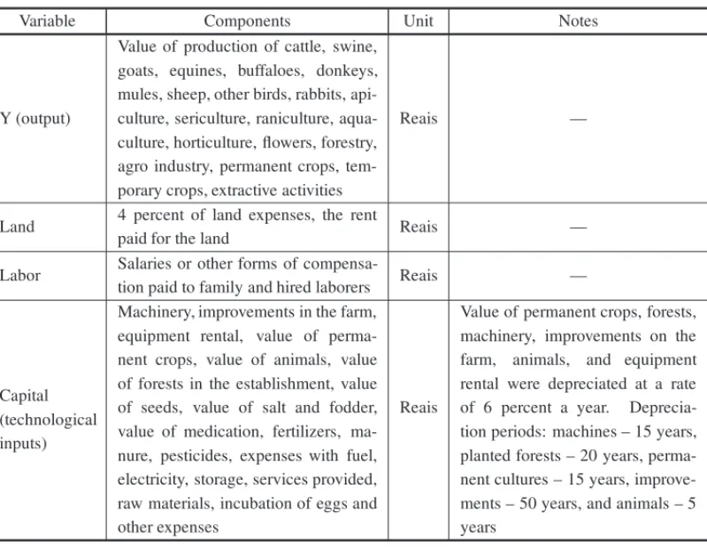
Table 1– Description of the production variables.
Variable Components Unit Notes
Y (output)
Value of production of cattle, swine, goats, equines, buffaloes, donkeys, mules, sheep, other birds, rabbits, api-culture, seriapi-culture, raniapi-culture, aqua-culture, hortiaqua-culture, flowers, forestry, agro industry, permanent crops, tem-porary crops, extractive activities
Reais —
Land 4 percent of land expenses, the rent
paid for the land Reais —
Labor Salaries or other forms of
compensa-tion paid to family and hired laborers Reais —
Capital (technological inputs)
Machinery, improvements in the farm, equipment rental, value of perma-nent crops, value of animals, value of forests in the establishment, value of seeds, value of salt and fodder, value of medication, fertilizers, ma-nure, pesticides, expenses with fuel, electricity, storage, services provided, raw materials, incubation of eggs and other expenses
Reais
Value of permanent crops, forests, machinery, improvements on the farm, animals, and equipment rental were depreciated at a rate of 6 percent a year. Deprecia-tion periods: machines – 15 years, planted forests – 20 years, perma-nent cultures – 15 years, improve-ments – 50 years, and animals – 5 years
Demographic dimension
The variables comprising the demographic dimension capture aspects of the population dynam-ics that relate to rural development. These are the proportion of the rural to the urban population, the average size of a rural family, the aging rate, the migration index, and the ratio of the inactive population (0 to 14 years and 60 years or more of age) to the active population (15 to 59 years of age). The data source is the Brazilian Demographic Census 2010 (IBGE, 2012b).
Environmental dimension
The variables comprising the environmental dimension are the proportion of farmers practicing the technique of vegetation fires, proportion of farmers who use agrochemicals, proportion of farmers practicing crop rotation, proportion of farmers practicing minimum tillage, proportion of farmers practicing no tillage, proportion of farmers planting in contour lines, proportion of farm-ers providing proper garbage disposal, proportion of forest and agro-forest areas, and proportion of degraded areas. The data source is the Brazilian Agricultural Census 2006 (IBGE, 2012a).
in the dimension, which in this case is the number of counties. Each specific dimension index is a weighted average of the normalized variables comprising the dimension, with weights defined by the relative squared multiple correlation obtained in the regression of a variable with all the others; that is, if Ri2 is the squared multiple correlation of the regression, considering theith variable as the dependent variable in the dimension, its weight isR2i/
j R 2 j.
3 FDH UNCONDITIONAL AND CONDITIONAL MEASURES OF TECHNICAL
EFFICIENCY
We begin with the notion of FDH efficiency and related measures. Daraio & Simar (2007) and B˘adin et al. (2012, 2014) discussed a measure of conditional efficiency that is closely relates FDH efficiency measures to probability theory, and which we used to assess the influence of covariates in the production process. Convexity of the technology set is not required. Consider production observations(xj,yj), j =1, . . . ,n, ofnproducing units (DMUs). In our case, the
input vectorxj =(x1j,x2j,x3j)is a vector inR3with non-negative components, representing the
land, labor, and capital components with at least one strictly positive. The output vectoryj is a
non-negative point inR. The technical efficiency FDH of DMUτ is taken relative to the frontier of free disposability (free disposal hull) of the set
ψ=
⎧ ⎨
⎩
(x,y)∈R+3+1,y≤
n
j=1
γjyj,x≥ n
j=1 γjxj,
n
j=1
γj =1, γj ∈ {0,1},j=1. . .n
⎫ ⎬
⎭
(1)
The input-oriented FDH efficiency measureθ (ˆ x,y)is given by
ˆ
θ (xτ,yτ)=Min
⎧ ⎨
⎩
θ;yτ ≤
n
j=1
γjyj, θxτ ≤
n
j=1 γjxj,
n
j=1
γj =1, γj ∈ {0,1}
⎫ ⎬
⎭
(2)
The output-oriented FDH efficiency measureλ(ˆ x,y)is given by
ˆ
λ(xτ,yτ)=Max
⎧ ⎨
⎩
λ;λyτ ≤
n
j=1
γjyj,xτ ≥
n
j=1 γjxj,
n
j=1
γj =1, γj ∈ {0,1}
⎫ ⎬
⎭
(3)
These quantities are similar to their DEA counterparts, including the interpretation of radial contraction (input orientation) and augmentation (output orientation). The main difference is that in DEA theγj are not restricted to be 0 or 1.
As stated in Dario & Simar (2007), the FDH estimator is computed in practice by a vector comparison procedure. In the case of three inputs and only one output, and assuming input ori-entation, we have
ˆ
θ (xτ,yτ)=Minj=1...n
Maxi=1,2,3
xij
xi
τ
For the output oriented FDH model we then have
ˆ
λ(xτ,yτ)=Maxj,xj≤xτ
y
j
yτ
. (5)
In this article we will restrict our attention to output oriented measures of efficiency (5).
A very interesting interpretation of the FDH arises when the production process is described by a probability measure, defined, in our case, in the product spaceR+3+1by random variables(X,Y). For efficiency purposes, we were interested in the probability of dominance given by
HX Y(y,x)=P(Y ≥ y,X ≤x). (6)
Notice that
1. HX Y(y,x) gives the probability that a unit operating at the input–output level(x,y)is
dominated, that is, that another unit produces at least as much output while using no more of any input than the unit operating at(x,y);
2. HX Y(y,x)is monotone non-decreasing inxand monotone non-increasing iny.
The support ofHX Y(x,y)is the technology setgiven by
HX Y(x,y)=0 ∀(x,y) /∈, (7)
where= {(x,y):xcan producey}.
We then have
HX Y(x,y)= P(X ≤x|Y ≥y)P(Y ≥y)=FX/Y(x|y)SY(y) (8)
HX Y(x,y)= P(Y ≥ y|X ≤x)P(X ≤x)=SY/X(y|x)FX(x). (9)
New concepts of efficiency measures can be defined for the input-oriented and output-oriented cases, assuming SY(y) > 0 and FX(x) > 0. For input and for output orientation we have,
respectively, the following equations
θ (x,y)=inf{θFX/Y (θx|y) >0} =inf{θ|HX Y (θx,y) >0} (10)
λ(x,y)=sup{λSY/X (λy|x) >0} =sup{λ|HX Y (λy,x) >0}. (11)
Since the support of the joint distribution of(X,Y)is the technology set, boundaries ofcan be defined in terms of conditional distributions.
As we stated before, in our empirical work we used the output orientation. The output efficiency measure for given levels of input(x)and output(y)is given in (11) and it is nonparametrically estimated by
ˆ
λn(x,y)=sup
λ
SˆY|X,n(λy|x) >0
where
ˆ
SY|X,n(y|x)=
n
i=1I(xi ≤x,yi ≥y)
n
i=1I(xi ≤x) .
It can be shown that the following equation coincides with the FDH estimator.
ˆ
λn(x,y)=Maxi:xi≤x y
i
y
. (13)
The estimated FDH production set is very sensitive to outliers, and consequently so are the es-timated efficiency scores. Here we avoided the outlier problem by transforming the data into ranks before the analysis. The approach is well known in statistics to produce methods that are robust relative to outlying and heteroskedastic observations. See Wonnacott & Wonnacott (1990) for Anova applications & Conover (1999) for a general discussion. In our case we experienced difficulties in computing performance measures using the raw data. For our purposes the rank transformation was sufficient to obtain directions of better performance. If a ranked dependent variable responds positively to a ranked independent variable, it is likely that the same relation-ship will occur for raw data. This is typical in regression problems.
To assess the significance of a continuous contextual variableZ of dimensionmon the output-oriented efficiency measurement, we conditioned onZ =zto obtain
λ(x,y|z)=sup{λ|SY (λy|x,z) >0}, where
SY(y|x,z)=Prob(Y ≥y|X ≤x,Z =z).
(14)
The nonparametric kernel estimate proposed by Daraio & Simar (2007) is defined by
ˆ
SY,n(y|x,z)=
n
i=1I(xi ≤x,yi ≥ y)Khn(Zi−z) n
i=1I(xi ≤x)Khn(Zi−z)
, (15)
whereK(·)is the kernel andhnis the bandwidth.
The bandwidth selection can be carried out using likelihood cross-validation as described by Silverman (1986), but other methods can also be used. For the multivariate case, we could use a bounded multivariate kernel or a product of univariate bounded kernels. An easy choice in the latter case would be the product of marginal kernels with support[−1,1]k. In our casek =6, which is the number of covariates.
Substituting the estimator SˆY,n(y|x,z)into equation (14), we obtained the conditional FDH
efficiency measure for the output-oriented case as below.
ˆ
λn(x,y|z)=sup{λ
SˆY (λy|x,z) >0}. (16)
Therefore, for a multivariate bounded kernel we used the following estimator
ˆ λn(xj,yj
zj)= max {i;xi≤xj,zi−zj≤τnσˆ}
yi
yj
whereτnis the bandwidth andσˆ is the square root of the average variance of the covariates.
With a product of univariate bounded kernels, following B˘adin et al. (2012), it is also possible to use the following formulation
ˆ λ(xj,yj
zj)= max i;xi≤xj,
z
1
i−z1j
≤τ1n,...,
z
m i −zmj
≤τmn
y i yj , (18)
where(τ1n, . . . , τmn)is the vector of marginal univariate bandwidths of the covariates.
The statistical inference will be dependent on how the kernels and bandwidths are chosen. Typically, nonparametric estimates are not dependent on the kernel choice and we proceed with the suggestion of Silverman (1986) and Daraio & Simar (2007), which is the Epanechnikov kernel. In our approach we obtained a better fit using a single bandwidth, also following Silver-man (1986) for the bandwidth choice. The multivariate Epanechnikov kernel is given by
K(u)=
(1/(2cd)) (d+2)(1−u′u) ifu′u<1
0 otherwise , (19)
whereu is a point in a d-dimensional space andcd is the volume of the unit sphere. In our
applicationd =6 andc6=(1/6)π3.
The optimal window width for the smoothing of normally distributed data with unit variance is given by
hopt =A(K)n−1/(d+4)
A(K)=
8c−d1(d+4)2√πd
1/(d+4) (20)
If the data are not transformed for unit variances, the indicated procedure is to choose a single-scale parameter σˆ and to use the value σˆhopt for the window width. A possible choice is
ˆ
σ2=d1d
i=1σˆi2as above, where(σˆ 2 1, . . . ,σˆ
2
d)is the vector of variances of the covariates.
4 STATISTICAL INFERENCE AND COVARIATE ASSESSMENT
For the assessment of the influence of the covariates on the efficiency measurements, Daraio & Simar (2007) suggested a nonparametric statistical analysis using the ratio
qn(xj,yj
zj)=
ˆ λn(xj,yj
zj) ˆ
λn(xj,yj)
as the response variable. The underlying suggested statistical model (Daraio & Simar, 2007) is E
q(xj,yj
zj) = G(µj), µj = z′jθ, assuming the vector of covariates to be exogenous.
variable is correlated with the error term. This problem seems to be more serious than the cross-sectional correlations. A similar condition is “separability,” which was discussed by Simar & Wilson (2007). The typical approach to overcome the problem of endogeneity is the instrumental variable estimation.
A natural parametric version of the model above is to consider the flexible fractional regression specification of Ramalho et al. (2010). We assumed that the observations are correlated and that some of the covariates are endogenous (the Gini index, financing, technical assistance, and social and environment indicators). The correlation is induced by the FDH computations.
A common choice forG(·)isG(µ) = (µ), where(·)denotes the distribution function of the standard normal. Other specifications could be the logisticG(µ)=eµ/(1+eµ)or the com-plementary log-logG(µ) = 1−e−eµ, but frequently they lead to similar conclusions. In our case we obtained the best response for the standard normal, followed by the logistic. The com-plementary log-log did not converge. Our preferred method of estimation was the generalized method of moments – GMM (Gallant, 1987; Greene, 2011), with robust estimation of the pa-rameter vector variance-covariance matrix. The GMM handles the problems of endogeneity and nonlinearity of the expected mean and, in many instances, provides robustness relative to the correlated observations as well (Conley, 1999; Stata, 2015).
Lethinst be a vector of strictly exogenous variables available for use as instruments. If
uj n(θ ,zj)= ˆ
λn(xj,yjzj) ˆ
λn(xj,yj)
−G(z′jθ )
and assuming the moment condition Eh⊗uj n(θ ,zj) = 0 to be true, we may estimate the
parameterθusing the generalized method of moments. An endogeneity and goodness-of-fit test is performed, testing for overidentifying restrictions (Hansen’s J test; Hansen, 1982).
To obtain bias-corrected confidence intervals and standard errors adjusted for all potential mis-specifications (endogeneity, cross-sectional correlation, and heteroskedasticity), we performed nonparametric bootstrapping (Stata, 2015) with 5,000 replications. The instruments that we chose here are regional dummies and variables measured after the agricultural census of 2006, available in the demographic census of 2010.
5 STATISTICAL FINDINGS
service in 2010, the demographic index, and demographic∧2. A standard procedure in GMM estimation is to also include as instruments low order monomials in the in the instrument set (Gallant, 1987). Standard errors were computed from the bootstrap replications. The Hansen’s J test statistic for the model correctness and instruments specification is 1.299, with 1 degree of freedom and p-value=0.254. There is no evidence against the model specification and the instruments considered.
Ratkowsky (1983) considered the bound 1% for the relative bias as the threshold for linear nor-mal behavior of a parameter estimator. Relative bias is defined as the ratio of the bias to the parameter estimate in absolute values. It is necessary to access the bootstrap distribution in order to estimate the relative bias. The 1% relative bias is achieved for the variables financing, social, demographic, and technical assistance. We failed to accept the normal assumption for the esti-mators of these parameters considering the bootstrap distribution. Only the Gini variable showed normal behavior. The Kolmogorov-Smirnov statistics of normality for financing, environment, social, demographic, technical assistance, and the Gini index are 0.014 (p-value = 0.0184), 0.028 (p-value< 0.01), 0.014 (p-value = 0.0186), 0.030 (p-value < 0.01), 0.020 (p-value
< 0.01), 0.038 (p-value < 0.01), and 0.007 (p-value > 0.15), respectively. In general, the distributions are skewed, and bias-corrected confidence intervals should be taken into account to assess the statistical significance. In this context, the environment and demographic variables are not significant.
Table 2– GMM estimation.
Relative Bootstrap Robust Robust SE/ 95% bootstrap Variable Estimate
bias standard standard Boot SE confidence
error error interval
Constant –2.7224 3.9017 1.0081 0.9903 0.9823 –4.6988 –0.6540
Financing 1.6870 0.5719 0.4904 0.5131 1.0463 0.8489 2.8144
Environment 1.3131 7.1068 1.1484 1.1800 1.0276 –0.8677 3.6785
Social 1.4740 0.9230 0.5705 0.5481 0.9608 0.4955 2.7652
Demographic 0.5780 0.0194 0.3407 0.3324 0.9758 –0.0659 1.2892
Tech. Assist. –2.7881 0.0087 0.8831 0.8507 0.9633 –4.8169 –1.3202
Gini 3.1425 3.2974 1.0285 0.9865 0.9592 1.0724 5.1064
The marginal effects were computed following the equation
d G(µ)
dµ θj|µ=z
′θ , d G(µ)
dµ =φ (µ), (21)
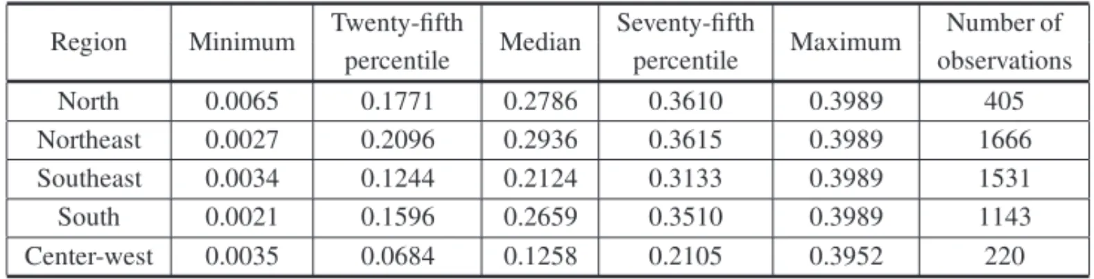
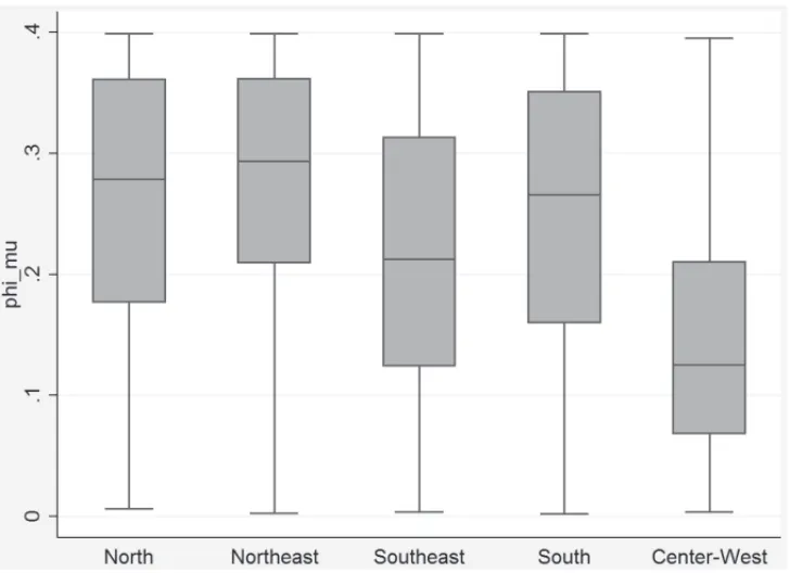
whereφ (·)is the standard normal density function. The intensity of the marginal effects on the response may be appreciated by the median values of the factorφ (µ). Table 3 shows five-number summaries for each region, and the corresponding box plots are shown in Figure 1. The region that will benefit the most from public policies reducing market imperfections,ceteris paribus, is the northeast, closely followed by the northern, southern, and southeastern regions.
Table 3– Five-number summary statistics for the regional marginal effects.
Region Minimum Twenty-fifth Median Seventy-fifth Maximum Number of
percentile percentile observations
North 0.0065 0.1771 0.2786 0.3610 0.3989 405
Northeast 0.0027 0.2096 0.2936 0.3615 0.3989 1666
Southeast 0.0034 0.1244 0.2124 0.3133 0.3989 1531
South 0.0021 0.1596 0.2659 0.3510 0.3989 1143
Center-west 0.0035 0.0684 0.1258 0.2105 0.3952 220
6 SUMMARY AND CONCLUSIONS
Figure 1– Regional marginal effects box plots.
was performed with instrumental variables, to handle the eventual endogeneity and separability problems, and bootstrapping, to address the cross-sectional correlation and heteroskedasticity properly.
We conclude that the market imperfections discriminate against the small rural producers. The public policies are directed to the rich farmers, since the interest rates are higher for the small producers, the leasing of equipment and machinery is also more expensive, access to health and education services is compromised, and the infrastructure drawbacks are more difficult to overcome. These conditions are unfavorable for production, making it impossible for small farms to adopt technologically intensive inputs. We also found a strong positive association between rural production efficiency and income concentration, emphasizing the difficulties faced by poor farmers in accessing proper technology at competitive prices due to market imperfections.
function as a proxy for the Gini quantity computed here. If the purpose of public policies is to reduce income concentration, one should invest in technologies that will increase land and labor productivity, and this cannot be achieved in the presence of market imperfections. In our study, we found that the northern and the northeastern regions in Brazil are likely to be the most responsive to marginal effects in income concentration and market imperfections. Therefore, public policies should be aimed at reducing the income concentration and creating conditions that allow productive inclusion and rural poverty reduction.
REFERENCES
[1] ALVESE & SOUZAGS. 2015. Pequenos estabelecimento em termos de ´area tamb´em enriquecem? Pedras e tropec¸os.Revista de Pol´ıtica Agr´ıcola,24(3): 7–21.
[2] ALVES E, SOUZA GS & ROCHA DP. 2013. Desigualdade nos campos sob a ´otica do censo agropecu´ario 2006.Revista de Pol´ıtica Agr´ıcola,22(2): 67–75.
[3] ALVESE, SOUZAGS, GARAGORRYFL & MELLOPF. 2015. O sonho de produzir: assentados da reforma agr´aria da Bahia e do Rio Grande do Sul.Revista de Pol´ıtica Agr´ıcola,24(3): 114–133.
[4] BADINL, DARAIOC & SIMARL. 2012. How to Measure the Impact of Environmental Factors in a Nonparametric Production.European Journal of Operations Research,223: 818–833.
[5] BADIN L, DARAIO C & SIMAR L. 2014. Explaining inefficiency in nonparametric production models: the state of the art.Annals of Operations Research,214(1): 5–30.
[6] BANKERRD, CHARNESA & COOPERWW. 1984. Some models for estimating technical scale inefficiencies in Data Envelopment Analysis.Management Science,30(9): 1078–1092.
[7] CONFEDERAC¸ ˜AO NACIONAL DA AGRICULTURA. 2013. ´Indice de Desenvolvimento Rural CNA. Bras´ılia: CNA (unpublished document).
[8] CONLEYTG. 1999. GMM estimation with cross sectional dependence.Journal of Econometrics,92: 1–45.
[9] CONOVERWJ. 1999. Practical Nonparametric Statistics. 3rd ed. New York: Wiley.
[10] DARAIOC & SIMARL. 2007. Advanced Robust and Nonparametric Methods in Efficiency Analysis. New York: Springer.
[11] DAVIDSONR & MACKINNONJG. 1993. Estimation and Inference in Econometrics. New York: Oxford University Press.
[12] EMBRAPA. 2001. Balanc¸o Social da Pesquisa Agropecu´aria Brasileira. Bras´ılia: Secretaria de Comunicac¸˜ao/Secretaria de Gest˜ao Estrat´egica.
[13] FERREIRACR & SOUZASCI. 2007. As aposentadorias e pens ˜oes e a concentrac¸˜ao dos rendimentos domiciliares per capita no Brasil e na sua ´area rural: 1981 a 2003.Revista de Economia e Sociologia Rural,45(4): 985–1011.
[14] GALLANTAR. 1987. Nonlinear Statistical Models. New York: Wiley.
[15] GREENEWH. 2011. Econometric Analysis. 7th ed. New Jersey: Prentice Hall.
[17] IBGE. 2012. Censo Agropecu´ario 2006. 2012a. Dispon´ıvel em: http://www.ibge.gov.br/ home/estatistica/economia/agropecuaria/censoagro/. Acesso em: 24 jan. 2012.
[18] IBGE. 2012. Censo Demogr´afico 2010. 2012b. Dispon´ıvel em: http://censo2010.ibge. gov.br/. Acesso em: 24 jan. 2012.
[19] INEP. 2012. Nota T´ecnica do ´Indice de Desenvolvimento da Educac¸˜ao B´asica. Dispon´ıvel em: http://ideb.inep.gov.br/resultado/. Acesso em: 24 jan. 2012.
[20] MINISTERIO DA´ SAUDE´ . 2011. IDSUS – ´Indice de Desempenho do SUS. Ano 1. Dispon´ıvel em: http://portal.saude.gov.br/. Acesso em: 02 mar. 2012.
[21] MONTEIRORC & RODRIGUESGS. 2006. A system of integrated indicators for socio-environmental assessment and eco-certification in agriculture – Ambitec-agro.Journal Technology Management & Innovation,1(3): 47–59.
[22] MOREIRATB, PINTOMB & SOUZAGS. 2004. Uma metodologia alternativa para mensurac¸˜ao de press˜ao sobre o mercado de cˆambio.Estudos Econˆomicos,34: 73–99.
[23] NEDERHD & SILVAJLM. 2004. Pobreza e distribuic¸˜ao de renda em ´areas rurais: uma abordagem de inferˆencia.Revista de Economia e Sociologia Rural,42(3): 469–486.
[24] NEY MG & HOFFMANNR. 2008. A contribuic¸˜ao das atividades agr´ıcolas e n˜ao-agr´ıcolas para a desigualdade de renda no Brasil rural.Economia Aplicada,12(3): 365–393.
[25] NEYMG & HOFFMANNR. 2009. Educac¸˜ao, concentrac¸˜ao fundi´aria e desigualdade de rendimentos no meio rural brasileiro.Revista de Economia e Sociologia Rural,47(1): 147–181.
[26] RAMALHOEA, RAMALHOJJS & HENRIQUESPD. 2010. Fractional regression models for second stage DEA efficiency analyses.Journal of Productivity Analysis,34: 239–255.
[27] RATKOWSKYDA. 1983. Nonlinear Regression Modeling, a unified practical approach. New York: Marcel Dekker.
[28] RODRIGUESGS, BUSCHINELLICCA & AVILAAFD. 2010. An environmental impact assessment system for agricultural research and development II: institutional learning experience at Embrapa.
Journal Technology Management & Innovation,5(4): 38–56.
[29] SILVERMANBW. 1986. Density Estimation. New York: Chapman and Hall.
[30] SIMARL & WILSONPW. 2007. Estimation and Inference in two-stage, semi-parametric models of production processes.Journal of Econometrics,136(1): 31–64.
[31] SOUZAGS & GOMESEG. 2015. Management of agricultural research centers in Brazil: a DEA application using a dynamic GMM approach.European Journal of Operational Research, 240: 81–824.
[32] SOUZAGS, GOMESEG & ALVESERA. 2015. Assessing the determinants of rural income disper-sion in Brazil.Anais do XLVII Simp´osio Brasileiro de Pesquisa Operacional, 582–591.
[33] SOUZAMO, MARQUESDV & SOUZAGS. 2013. Uma metodologia alternativa para c´alculo dos indices de impactos sociais e ambientais das tecnologias da Embrapa.Cadernos do IME-S´erie Estat´ıstica,34: 1–15.
[34] STATA. 2015. Base Reference Manual Release 14. Texas: Stata Press.