http://www.uem.br/acta ISSN printed: 1679-9275 ISSN on-line: 1807-8621
Doi: 10.4025/actasciagron.v37i4.19766
Agrometeorological models for groundnut crop yield forecasting in
the Jaboticabal, São Paulo State region, Brazil
Victor Brunini Moreto* and Glauco de Souza Rolim
Faculdade de Ciências Agrárias e Veterinárias, Universidade Estadual “Julio de Mesquita Filho”,Via de Acesso Prof.Paulo Donato Castellane s/n.º, 14884-900, Jaboticabal, São Paulo, Brazil. *Author for correspondence. E-mai: [email protected]
ABSTRACT. Forecast is the act of estimating a future event based on current data. Ten-day period (TDP) meteorological data were used for modeling: mean air temperature, precipitation and water balance components (water deficit (DEF) and surplus (EXC) and soil water storage (SWS)). Meteorological and yield data from 1990-2004 were used for calibration, and 2005-2010 were used for testing. First step was the selection of variables via correlation analysis to determine which TDP and climatic variables have more influence on the crop yield. The selected variables were used to construct models by multiple linear regression, using a stepwise backwards process. Among all analyzed models, the following was notable: Yield = - 4.964 x [SWS of 2° TDP of December of the previous year (OPY)] – 1.123 x [SWS of 2° TDP of November OPY] + 0.949 x [EXC of 1° TDP of February of the productive year (PY)] + 2.5 x [SWS of 2° TDP of February OPY] + 19.125 x [EXC of 1° TDP of May OPY] – 3.113 x [EXC of 3° TDP of January OPY] + 1.469 x [EXC of 3 TDP of January of PY] + 3920.526, with MAPE = 5.22%, R2 = 0.58 and
RMSEs = 111.03 kg ha-1.
Keywords: crop model, water balance, prediction, production.
Modelos agrometeorológicos para previsão de produtividade de amendoim na região de
Jaboticabal, Estado de São Paulo, Brasil
RESUMO. Previsão é o ato de estimar a partir de dados atuais um acontecimento futuro. Os dados meteorológicos decendiais utilizados para modelagem foram: temperatura média do ar, precipitação e componentes de balanço hídrico como deficiência (DEF), excedentes (EXC) hídricos e armazenamento de água no solo (SWS). Dados meteorológicos e de produtividade entre 1990-2004 foram utilizados para calibração e 2005-2010 para teste. Primeiramente foi realizada a seleção de variáveis por meio de análise de correlação, evidenciando quais decêndios e quais variáveis climáticas, influenciam mais diretamente a produtividade. Com as variáveis escolhidas, foram construídos modelos com regressão linear múltipla utilizando processo “stepwise backwards”. Dentre todos os modelos analisados, destaca-se: Produtividade = - 4,964 x [SWS do 2° DEC de dezembro do ano anterior (OPY)] - 1,123 x [SWS do 2° DEC de novembro OPY] + 0,949 x [EXC do 1° DEC de fevereiro do ano produtivo] + 2,5 x [SWS do 2° DEC de fevereiro OPY] + 19,125 x [EXC do 1° DEC de maio OPY] - 3,113 x [EXC do 3° DEC de janeiro OPY] + 1,469 x [EXC do 3° DEC de janeiro do ano produtivo] + 3920,526, com MAPE = 5,22%, R2 = 0,58 e RMSEs = 111,03 kg ha-1.
Palavras-chaves: modelo de cultivo, balanço hídrico, predição, produção.
Introduction
The groundnut, one of the major oilseeds produced in the world, belongs to the family Leguminosae. The plant has a high energy value, is rich in nutrients and is use to produce a wide range of products derived from the grain, like oil such as peanut butter and ‘in natura’ peanut (FREITAS et al., 2005).
According to the National Supply Company (CONAB, 2012), the Brazilian production in 2010/2011 compared to 2009/2010, was reduced by 32%, with a 12% reduction in the planted area. These reductions were mainly caused by climatic
factors, such as excessive rainfall at the end of the peanut crop cycle.
São Paulo, and the Jaboticabal region in particular, accounts for almost 70% of the entire Brazilian product. This region is distinguished by their average yield, of 3.7 ton. ha-1, which is much
higher than the national average of 2,8 t ha-1 and the
global average of 1.6 ton. ha-1 (IEA, 2011).
analysis of the errors involved. An alternative subjective method is the use of crop models, known as agrometeorological models which express the influence of meteorological elements on crop yield.
According to Rossetti (2001), 95% of claims paid by agricultural security entities are related to drought or excess rain. Modeling is a mean to quantify these climates risks, estimate yields and devise strategies to minimize their impacts in a rapid and cost-effective manner.
In São Paulo, the recommended groundnut sowing date, consider climatic condition of each region. Generally, the months of October and November are the most suitable to sowing the groundnut known as the “water crop”. The “dry crop” is typically sowed in February (GODOY et al., 1986).
The groundnut cycle ranges from 90 to 115 days for early varieties and from 120 to 140 days for late varieties. Depending on the weather the water requirements range from 500 to 700 mm for both cycles (DOORENBOS; KASSAM, 1979). According to Silva and Rao (2006), in general, water deficits during the growing season cause flowering delays and extend the crop cycle, thereby delaying harvest and reducing yield. The phase of flowering and pod formation is highly sensitive to water stress. The harvest must be performed in the appropriate season. Harvests at an unsuitable time may lead to considerable losses, both in the quantity and quality of seeds. Earlier harvests result in considerable quantities of immature and poorly formed seeds, whereas late harvests can lead to the greater deterioration of seeds (CARVALHO et al., 1976). Soil moisture can severely damage and reduce the quality of the seeds, most likely because of the occurrence of rain (TOLEDO; MARCOS FILHO, 1977); subsequent to harvest, seed germination may occur with the pod (SAVY FILHO; LAGO, 1985), resulting in the deterioration of the seeds during storage.
Studies of the water balance should be developed to facilitate an understanding of the relationship between culture and climate, which allows for an adjustment of the crop climatic conditions, thereby avoiding disastrous consequences of defective agricultural planning (TUBELIS, 1988). The main climate elements, according to Ometto (1981) and Vianello and Alves (1991), are the precipitation, air temperature, solar radiation, atmospheric moisture, wind and atmospheric pressure.
Doorenbos and Kassam (1979) reported that, to obtain a high yield, a rainfed crop requires approximately 500 to 700 mm of water for the entire period of growth. The indices of drought sensitivity (Ky) for the phases of establishment, vegetative
growth, flowering and maturity are 0,2; 0,2; 0,8 and 0,6 respectively, indicating that the flowering period is more sensitive to water deficit (DOORENBOS; KASSAM, 1979).
Groundnuts grow well in environments with average daytime temperatures between 22°C and 28°C (CRAUFURD et al., 2002; DOORENBOS; KASSAM, 1979). The period from sowing to flowering requires 313 GDD (growing degree days) to 360 GDD, depending on the variety (KETRING; WHELESS, 1989).
According to Robertson (1983) yield-climate interactions can be quantified using models and studying the variations and effects of climate on plant performance.
Agricultural simulation models can be understood as empirical or mechanistic mathematical equations that aim to simplify reality and represent the biomass accumulation and plant development as well as estimate their yield according to the influencing factors. Empirical models are those based on regression analyses, whereas mechanistic models quantify and seek to understand the physical and biological interactions of plants with their development and environment (ZHU, 2010).
The knowledge of the space-temporal variability of long-term series of meteorological data can assist in the identification of better areas and periods for sowing for the crops, as well as provide important information on possible climatic trends. The union of the knowledge of space-temporal variability is a fundamental step for reducing climatic risks associated with the agricultural sector (BLAIN, 2009).
Few agrometeorological models are available to estimate the yields of groundnut crops (ESPOSTI, 2002; MARIN et al., 2006). Assunção and Escobedo (2009) developed a model to estimate the crop yield as a function of the water availability. However, as mentioned above, most models estimate but do not forecast the yield. For example, Challinor et al. (2003) indicated that yield estimations and forecasting can be improved if we relate crop models to weather forecasting.
This study aimed to identify the climatic elements in ten-day dataset that influence the annual groundnut yield in the Jaboticabal region. The other objective was to develop agrometeorological model (s) for regional groundnut yield forecasting.
Material and methods
Agrometeorological Station of the Department of Exacts Science - FCAV/Unesp, Jaboticabal, located at latitude 21°14’05’’, longitude 48°17’09’’ and an altitude of 600 m.
The mean air temperature and precipitation were used for estimating the ten-day period (TDP) reference evapotranspiration (ETo) according to the Thornthwaite (1948) method. The components of the water balance (WB) proposed by Thornthwaite and Mather (1955), such as the deficit (DEF), water surplus (EXC) and soil storage water (SWS) were calculated using an available water capacity (AWC) of 100 mm.
The groundnut production data were obtained from the Institute of Agricultural Economy (IEA) for a period of 20 years, from 1990 to 2010. The yield data were adjusted as proposed by Prela-Pantano et al. (2011), to remove the technological trend. This adjustment is necessary to minimize effects due to changes in the technological level employed by producers, thereby obtaining the influence of the climate variability on the yield.
A linear correlation analysis (r, Pearson) was performed using a TDP of SWS, DEF and EXC of the harvest year and the same elements of the previous year. The variables with the best correlations were selected for modeling. The models were constructed by multiple linear regression (Y = a.X1 + b.X2 + c.X3 + … + LC)
where Y is the yield of the harvest year, the independent variables are the climatic elements and LC is the linear coefficient.
In modeling, especially with the use of many independent variables, the main problem is the selection and combination of the variables. A stepwise backwards regression method was used, based on the criterion of accuracy (R2 adjusted)
improvement. A total of 511 regressions were obtained and analyzed by combinatory analysis. Only models shaving at least 0,05 significance (P value) in the parameters and in the regression were selected.
After this step, 28 models were chosen for the region. These models were evaluated using an accuracy analysis based on the mean absolute percentage error (MAPE), precision analysis based on the adjusted coefficient of determination (R2)
and tendency analysis based on the Root Mean Systematic Error (RMSEs) (Equations 1, 2 and 3, respectively). We used a 14 year period (1990 to 2004) for the model calibration and a 6 year period (2005 to 2010) for testing (or validation).
= ∑
− × 100
(1)
² = 1 − 1 − ² ×− − 1− 1 (2)
= ∑ − (3)
where:
Yesti: estimation of year ‘i’ yield; Yobsi:
observed yield (without technological trend) in year ‘i’; YestC: yield estimated by simple linear
regression between the observed (Yobsi) and
estimated (Yesti) yield; N: number of years; n:
number of data and k: number of independent variables in the regression.
Results and discussion
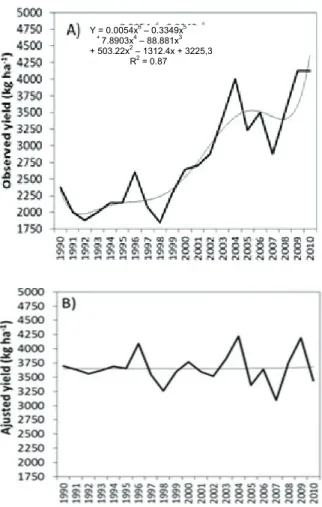
The period of analysis showed a wide variability in the crop yield (Figure 1A). This irregularity occurred due to climate variables and changes in the level of technology that was available. A 6° order polynomial adjustment was applied to minimize the effects of the agricultural technology level that was used (Figure 1A) and to clearly demonstrate the effects of climate on the crop yield. The adjusted yields (Figure 1B) are used throughout the remainder of the paper.
The occurrence of heavy rainfall in 1992/1993 season (Figure 2), and the lack of heavy rain in the 1991/1992 season during the final phases of crop development (flowering and fructification) had a considerable negative effect on the groundnut yields in those years. According to Gillier and Silvestre (1996), groundnut flowering and fructification are dependent on certain climatic elements, and a change in the water availability directly and intensely affects the crop yield.
Figure 1. Groundut observed yield (A) and adjusted yield to remove the technological trend (B), in Jaboticabal, São Paulo State, from 1990 to 2010.
Figure 2. Sequencial anual water balance at Jaboticabal, SP, by the model of Thornthwaite and Mather (1955) with available water capacity of 100 mm in the period of 1990 to 2010.
The 2004 season (Figure 4) had the highest yield due to the occurrence of large EXC between January and February at the appropriate times (flowering and fructification) and DEF between March and December favoring the maturation and harvest of the crop.
A correlation analysis was performed to select elements of the water balance (WB) within the ten-day period (TDP) (independent variables)
that had the greatest influence on the crop yield (Table 1). These selected variables were used to construct the agrometeorological models.
Figure 3. Ten-day period sequential water balance by the method of Thornthwaite and Mather (1955) with available water capacity of 100 mm of the season 1997/1998
Figure 4. Ten-day period sequential water balance by the method of Thornthwaite and Mather with available water capacity of 100 mm of the season 2003/2004.
Table 1. Selected coefficient of correlation (r) among the most important meteorological variables and yield. Legend: X1: soil
water storage (SWS) of the 2° TDP of December of the previous year (OPY); X2: SWS of the 2° TDP of November OPY; X3:
water surplus (EXC) of the 1° TDP of February; X4: SWS of the
2° TDP of February OPY; X5: water deficit (DEF) of the 2° TDP
of December; X6: EXC of the 1° TDP of May OPY; X7: EXC of
the 3° TDP of January OPY; X8: EXC of the 3° TDP of January;
X9: yield OPY.
PROD X9 X1 X2 X3 X4 X5 X6 X7 X8
PRO
D 1
X9 0.840 1
X1 -0.477 -0.213 1
X2 -0.448 -0.333 0.451 1
X3 -0.438 -0.417 0.348 0.445 1
X4 0.449 0.278 -0.355 -0.239 -0.362 1
X5 0.452 0.414 0.185 0.012 0.000 0.209 1
X6 0.561 0.361 -0.732 -0.480 -0.212 0.210 0.000 1
X7 0.674 0.687 -0.359 -0.402 -0.034 0.255 0.000 0.613 1
X8 0.701 0.618 -0.290 -0.233 0.000 0.337 0.000 0.406 0.469 1
In the calibration, the models ‘1’ to ‘7’ (Tables 2 and 3) showed the high accuracies having MAPE values found of less than 3,25%. Considering the average yield in the region of 2780 kg ha-1, the observed MAPE corresponds to
90 kg ha-1, or 1.5 sacks of 60 kg ha-1. The
independent variable X6, which represents the
EXC of the 1° TDP of the May OPY, was important in all models, except model ‘5’. This Y = 0.0054x6 – 0.3349x5
+ 7.8903x4 – 88.881x3
+ 503.22x2 – 1312.4x + 3225,3
importance can be explained by the fact that the timing of the end of maturation and early harvest period coincides with this variable (Figure 5).
The models were also evaluated with respect to their ability to forecast yields prior to the harvest or before the crop sowing. For this reason, the first four models (Table 2) are most interesting for discussion. The models not only present the best accuracy (MAPE) but they also ignore the variable X5; therefore these models can forecast the yield
prior to the sowing date. Whenever possible the variable X5, should be discarded because it uses
the 2° TDP of December of the productive year, thereby preventing a forecast of the yield.
The second step of the study was to test the selected models using independent data from the period of 2005 to 2010. The first eight models showed high accuracy (Table 3), high precision and low tendency, as evidenced by, MAPE values less than 8,25%, a minimum R2 of 0.56 and a
minimum RMSEs of 110.86 kg ha-1.
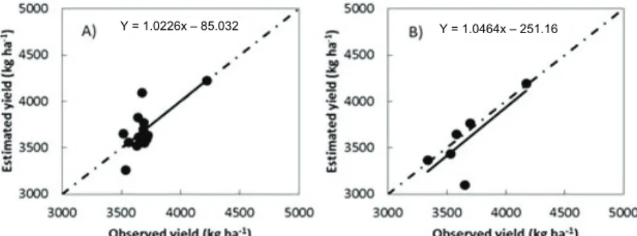
Among the top four models (Tables 2 and 3), model ‘1’ showed the best accuracy in the tests, with a MAPE of 0.99% and precision (R2) of 0.6
(Figure 6b). This model is interesting because it uses just four variables: X6, X7, X8 and X9 (Table
2). These variables are related to the EXC of 3° TDP of January of the same year and the EXC of the 3° TDP of January and the 1° TDP of May OPY. According to Silva and Rao (2005), this result confirms that in January, the crop is generally at the beginning of the flowering phase, which requires the greatest water supply (Figure 5).
Models ‘3’ and ‘4’ showed good accuracy with MAPE values of 5.22% and 5.73%, respectively. In both models the variable X9 (Table 2) was not
used, so it is possible to forecast the yield using only meteorological data.
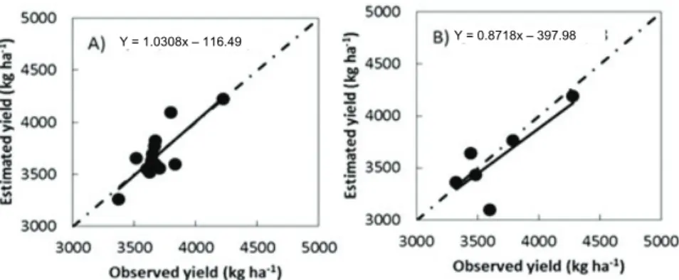
Finally, the following models were found to have both high accuracy and high applicability: model ‘1’ (Yield = 23.341.X6 - 2.315.X7 +
0.898.X8 – 0.092.X9 + 4010.508), model ‘2’ (Yield
= -5.199.X1 - 1.118.X2 + 0.931.X3 + 2.284.X4 +
18.641.X6 – 2.997.X7 + 1.511.X8 – 0.033.X9 +
4076.521) and model ‘3’ (Yield = - 4.964.X1 –
1.123.X2 +0.949.X3 + 2.5.X4 +19.125.X6 –
3.113.X7 +1.469.X8 + 3920.526). These models
presented better statistical indices in both, the calibration and tests (Table 3) due to the lower dispersion of the estimate data relative to the observed data (Figures 6, 7 and 8).
Table 2. Coefficients of the agrometeorological models related to linear regression models (Y= a.X1+b.X2+c.X3+…+LC) for yiled
forecasting of groundnut crop at Jaboticabal region. Legend: X1: soil water storage (SWS) of the 2° TDP of December of the previous year
(OPY); X2: SWS of the 2° TDP of November OPY; X3: water surplus (EXC) of the 1° TDP of February; X4: SWS of the 2° TDP of
February OPY; X5: water deficit (DEF) of the 2° TDP of December; X6: EXC of the 1° TDP of May OPY; X7: EXC of the 3° TDP of
January OPY; X8: EXC of the 3° TDP of January; X9: yield OPY.
Models CL X1 X2 X3 X4 X5 X6 X7 X8 X9
1 4010.508 24.341 -2.315 0.898 -0.092
2 4076.521 -5.199 -1.118 0.931 2.284 18.641 -2.997 1.511 -0.033
3 3920.526 -4.964 -1.123 0.949 2.500 19.125 -3.113 1.469
4 3899.059 -3.995 -1.249 0.702 2.511 23.413 -2.745
5 5434.651 -10.798 -1.193 0.904 0.039 1.667 -1.510 2.824 -0.231
6 4784.275 -12.168 -0.838 0.534 0.305 41.591 -0.826
7 4480.624 -10.542 -1.074 1.007 1.185 12.395 -2.046 2.513
8 4908.069 -8.672 0.802 0.132 -0.205 52.648 18.333 -0.752 -0.134
9 3465.854 -0.761 0.640 2.990 42.965 30.123 -3.419
10 4312.806 -6.772 -0.413 0.629 53.634 23.893 -2.671
11 4047.005 -5.837 -0.190 0.727 1.975 51.380 25.110 -2.920
12 4315.315 -6.653 -0.323 0.557 59.531 25,474 -2.583 -0.462
Models CL X1 X2 X3 X4 X5 X6 X7 X8 X9
13 4042.558 -5.922 0.705 2.011 52.096 25.186 -2.889
14 3488.693 -0.653 0.554 2.902 50.120 31.845 -3.298 -0.542
15 4054.817 -5.770 -0.128 0.671 1.931 55.847 26.267 -2.849 -0.346
16 4052.306 -5.821 0.654 1.952 56.547 26.377 -2.825 -0.363
17 4067.099 -5.182 0.734 1.305 65.808 28.241 -2.288 -1.160
18 4340.557 -8.247 1.190 0.056 0.323 66.203 21.096 -1.482
19 3784.168 -6.193 -0.199 0.525 73.683 28.838 -2.911 -1.101 0.140
20 3040.384 -4.741 -0.038 0.898 3.327 59.072 27.757 -3.784 0.217
21 2907.719 85.647 38.034 -3.208 -2.210 0.241
22 2263.049 -3.258 0.773 4.112 88.946 36.286 -4.166 -1.948 0.396
23 2167.824 -3.329 0.477 0.715 4.295 93.115 37.170 -4.142 -2.090 0.414
24 2036.459 3.577 95.696 40.333 -3.824 -2.982 0.409
25 2278.374 -2.831 1.362 3.507 101.778 38.704 -3.480 -2.866 0.393
26 1518.384 0.718 5.179 96.275 41.723 -4.688 -2.495 0.501
27 1429.390 0.381 0.671 5.344 99.730 42.523 -4.678 -2.619 0.518
Table 3. Accuracy by the mean absolute percentage error (MAPE), precision by adjusted coefficient of correlation (R2) and tendency by
systematic root mean squared error (RMSEs) for the agrometeorological models presented in Table 2. The phase of calibration used data from 1990 to 2004 and test with 2005 to 2010.
Calibration Test
Models MAPE (%) Ajusted R2
RMSEs (kg ha-1
) MAPE (%) Ajusted R2
RMSEs kg ha-1
)
1 3.07 0.56 103.74 0.99 0.60 159.44
2 2.80 0.70 72.13 5.18 0.61 110.86
3 2.79 0.70 72.24 5.22 0.58 111.03
4 2.94 0.66 80.43 5.73 0.59 123.62
5 2.84 0.58 98.60 6.10 0.61 151.55
6 3.25 0.47 126.28 6.42 0.68 194.09
7 3.09 0.56 104.40 7.12 0.56 160.46
8 2.65 0.63 87.72 8.10 0.65 134.82
9 2.56 0.71 68.30 8.21 0.32 104.98
10 2.39 0.02 59.30 8.23 0.46 91.14
11 2.45 0.03 55.22 8.66 0.51 84.88
12 2.40 0.75 58.83 8.75 0.50 90.41
13 2.44 0.77 55.29 8.79 0.44 84.97
14 2.55 0.72 95.84 8.80 0.30 147.59
15 2.44 0.77 54.96 9.03 0.44 84.47
16 2.44 0.77 54.99 9.14 0.52 84.52
17 2.39 0.74 62.37 10.11 0.37 95.86
18 2.64 0.62 89.52 10.18 0.47 137.58
19 2,41 0.76 57.00 10.78 0.33 87.61
20 2.30 0.79 50.63 11.00 0.22 77.81
21 2.55 0.69 74.09 12.64 0.13 113.88
22 2.31 0.81 45.20 14.74 0.10 69.48
23 2.29 0.81 44.84 15.40 0.09 68.91
24 2.48 0.75 58.66 15.45 0.07 90.16
25 2.37 0.78 53.24 16.21 0.08 81.83
26 2.37 0.80 48.52 16.33 0.04 74.58
27 2.36 0.80 48.29 16.88 0.04 74.22
28 2.02 0.81 44.84 25.67 0.09 68.91
The variable X6 (EXC of the 1° TDP of May
OPY) had the greatest influence in all of the models because the adjusted parameter had a higher value than the other variables. The variable X7 (EXC of the 3° TDP of January OPY) was also
important because it was used in all selected models. This variable showed an inverse relationship with the water crop groundnut yield, indicating that excess water is moderately harmful in flowering and fructification. The X1 (SWS of
the 2° TDP of December OPY) also showed inverse relationship with yield, suggesting that water storage during vegetative growth should not be excessively high. These considerations are shown in Figure 5 for both water and dry crops.
Figure 5. Meteorological variables selected in the models 1, 2 and 3 and the periods of their influence on the water and dry crops of groundnut. Legend: water surplus (EXC), water deficit (DEF) and soil water storage (SWS).
Figure 6. Calibration of the parameters of model ‘1’ using ten-day period data of 1991 to 2004 (A) and test of the parameters, 2005 to 2010 (B).
Figure 7. Calibration of the parameters of model ‘2’ using ten-day period data of 1991 to 2004 (A) and test of the parameters, 2005 to 2010 (B).
Figure 8. Calibration of the parameters of model ‘3’ using ten-day period data of 1991 to 2004 (A) and test of the parameters, 2005 to 2010 (B).
Conclusion
The results showed that the following meteorological elements had the greatest influence of the groundnut yield at Jaboticabal: a) soil water storage of a 2° ten-day period (TDP) of February, November and December of the previous year (OPY); and b) water surplus of the 3° TDP of January and 1° TDP of May OPY before the seasonal year and the 3° TDP of January and 1° TDP of February of the seasonal year.
Models ‘1’, ‘2’ and ‘3’ were the most accurate. Model ‘3’ uses only meteorological data and, thus does not require using the yield OPY in its calculations.
References
ASSUNÇÃO, H. F.; ESCOBEDO, J. F. Use of an agrometeorological to computing the peanut water requirements. Revista Irriga, v. 14, n. 3, p. 325-335, 2009.
BLAIN, G. C. Statistical considerations of eight monthly precipitations series of the state of São Paulo, Brazil.
Revista Brasileira de Meteorologia, v. 24, n. 1, p. 12-23, 2009.
CARVALHO, N. M.; BUENO, C. R.; SANCHEZ, L. C. Maturação de sementes de amendoim (Arachis hypogaea L.).
Científica, v. 4, n. 1, p. 39-42, 1976.
CHALLINOR, A. J.; SLINGO, J. M.; WHEELER, T. R.; CRAUFURD, P. Q.; GRIMES, D. I. F. Toward a combined seasonal weather and crop yield forecasting system: Determination of the working spatial scale. Journal of Applied Meteorology, v. 42, n. 2, p. 175-192, 2003.
CONAB-Companhia Nacional de Abastecimento. Amendoim total (1a. e 2a. safra). Acompanhamento da safra brasileira de grãos. Brasília: CONAB, 2012. p. 10-13. CRAUFURD, P. Q.; PRASAD, P. V. V.; SUMMERFIELD, R. J. Dry matter production and rate of change of harvest index at high temperature in peanut. Crop Science, v. 42, n. 1, p. 146-151, 2002.
DOORENBOS, J.; KASSAM, A. H. Yield response to water. Rome: FAO, 1979. (Irrigation and Drenage, Paper 33).
ESPOSTI, M. D. D. Estimativa da perda de produtividade potencial do amendoim (Arachis hypogaea L.) e épocas de plantio na Região Sul do Espírito Santo em função do déficit hídrico. Revista Ciência Agronômica, v. 33, n. 2, p. 5-12, 2002.
FREITAS. M.; MARTINS, S. S.; NOMI, A. K.; CAMPOS, A. F. Evolução do mercado brasileiro de amendoim. In: SANTOS, R. C. (Ed.). O Agronegócio do amendoim no Brasil. Campina Grande: Embrapa, 2005. p. 16-44.
GILLIER, P.; SILVESTRE, P. Green and chicken manures for the peanut crop (Arachis hypogeae L.).
Scientia Agricola, v. 53, n. 1, p. 88-93, 1996.
GODOY, I. J.; RODRIGUES FILHO, F. S. O.; GERIN, M. A. N. Amendoim. In: Instituto Agronômico (Campinas). Instruções Agrícolas para o Estado de São Paulo.3. ed. Campinas: IAC, 1986. p. 23. (Boletim, 200). IEA-Instituto de Economia Agrícola. Previsões e estimativas das safras agrícolas do estado de São Paulo, ano agrícola 2010/2011. Informações Econômicas. São Paulo: IEA, 2011. v. 41, n. 4.
KETRING, D. L.; WHELESS, T. G. The Degree-day requirements for phenological development of peanut.
Agronomy Journal, v. 81, n. 1, p. 910-917, 1989.
MARIN, F. R.; PEZZOPANE, J. R. M.; PEDRO JÚNIOR, M.; GODOY, I. J.; GOUVÊA, J. R. R. F. Estimativa da produtividade e determinação das melhores épocas de semeadura para a cultura do amendoim no Estado de São Paulo. Revista Brasileira de Agrometeorologia, v. 14, n. 1, p. 64-75, 2006.
OMETTO, J. C. Bioclimatologia vegetal. São Paulo: Agronômica Ceres, 1981.
PRELA-PANTANO, A.; DUARTE, A. P.; SILVA, D. F.; ROLIM, G. S.; CASER, D. V. Yield of maize, and occurrence of enso precipitation in the region of the middle Paranapanema, SP, Brazil. Revista Brasileira de Milho e Sorgo, v. 10, n. 2, p. 146-157, 2011.
ROBERTSON, G. W. Guidelines on crop-weather models. Geneva: WMO, 1983. (World Climate Application Programme, 50)
ROSSETTI, L. A. Zoneamento agrícola em aplicações de crédito e seguridade rural no Brasil: aspectos atuariais e de política agrícola. Revista Brasileira de Agrometeorologia, v. 9, n 3, p. 386-399, 2001.
SAVY FILHO, A.; LAGO, A. A. Efeito da época de colheita na qualidade de sementes de amendoim. Revista de Agricultura, v. 60, n. 2, p. 11-16, 1985.
SILVA, L. C. L.; RAO, V. R. T. Evaluation of methods for stimating the peanut crop coefficients. Revista Brasileira de Engenharia Agrícola e Ambiental, v. 10, n. 1, p. 128-131, 2006.
THORNTHWAITE, C. W. An approach towards a rational classification of climate. Geographical Review, v. 38, n. 1, p. 55-94, 1948.
THORNTHWAITE, C. W.; MATHER, J. R. The water balance. drexel institute of technology. Laboratory of Climatology, v. 8, n. 1, p. 1-104, 1955.
TOLEDO, F. F.; MARCOS FILHO, J. Manual das sementes: tecnologia de produção. São Paulo: Agronômica Ceres, 1977.
TUBELIS, A. Chuva e a produção agrícola. Sao Paulo:
Nobel, 1988.
VIANELLO, R. L.; ALVES, A. R. Meteorologia básica e aplicações. Viçosa, UFV, 1991.
ZHU, X. G.; ZHANG, G. L.; THOLEN, D.; WANG Y.; CHIN, C. P.; SONG, Q. F. The next generation models for crops and agro-ecosystems. Science China Press, v. 54, n. 3, p. 589-597, 2011.
Received on February 5, 2013. Accepted on June 14, 2013.