www.atmos-meas-tech.net/9/3921/2016/ doi:10.5194/amt-9-3921-2016
© Author(s) 2016. CC Attribution 3.0 License.
HDO and H
2
O total column retrievals from TROPOMI shortwave
infrared measurements
Remco A. Scheepmaker1, Joost aan de Brugh1, Haili Hu1, Tobias Borsdorff1, Christian Frankenberg2, Camille Risi3, Otto Hasekamp1, Ilse Aben1, and Jochen Landgraf1
1SRON Netherlands Institute for Space Research, Utrecht, the Netherlands
2Jet Propulsion Laboratory (JPL), California Institute of Technology, Pasadena, CA, USA 3Laboratoire de Météorologie Dynamique, Insitut Pierre Simon Laplace, CNRS, Paris, France Correspondence to:Jochen Landgraf (j.landgraf@sron.nl)
Received: 2 April 2016 – Published in Atmos. Meas. Tech. Discuss.: 8 April 2016 Revised: 29 June 2016 – Accepted: 4 July 2016 – Published: 23 August 2016
Abstract. The TROPOspheric Monitoring Instrument
(TROPOMI) on board the European Space Agency Sentinel-5 Precursor mission is scheduled for launch in the last quarter of 2016. As part of its operational processing the mission will provide CH4 and CO total columns using backscattered sunlight in the shortwave infrared band (2.3 µm). By adapting the CO retrieval algorithm, we have developed a non-scattering algorithm to retrieve total column HDO and H2O from the same measurements under clear-sky conditions. The isotopologue ratio HDO/H2O is a powerful diagnostic in the efforts to improve our understanding of the hydrological cycle and its role in climate change, as it provides an insight into the source and transport history of water vapour, nature’s strongest greenhouse gas. Due to the weak reflectivity over water surfaces, we need to restrict the retrieval to cloud-free scenes over land. We exploit a novel 2-band filter technique, using strong vs. weak water or methane absorption bands, to prefilter scenes with medium-to-high-level clouds, cirrus or aerosol and to significantly reduce processing time. Scenes with cloud top heights.1 km, very low fractions of high-level clouds or an aerosol layer above a high surface albedo are not filtered out. We use an ensemble of realistic measurement simulations for various conditions to show the efficiency of the cloud filter and to quantify the performance of the retrieval. The single-measurement precision in terms of δD is better than 15–25 ‰ for even the lowest surface albedo (2–4 ‰ for high albedos), while a small bias remains possible of up to ∼20 ‰ due to remaining aerosol or up to ∼70 ‰ due to remaining cloud contamination. We also present an analysis
1 Introduction
Water vapour, being the strongest natural greenhouse gas, plays a vital role in our understanding of climate change. It is part of a positive atmospheric feedback mechanism (So-den et al., 2005; Randall et al., 2007), and it plays a role in the mechanisms of cloud formation, of which the feed-back mechanisms are still poorly understood (Boucher et al., 2013). A correct understanding of the many interacting pro-cesses that control atmospheric humidity, as well as con-straining atmospheric circulation, is crucial for general cir-culation models (GCMs) to come to accurate climate projec-tions (Jouzel et al., 1987; Yoshimura et al., 2011, 2014; Risi et al., 2012a, b).
Measurements of stable water isotopologues, such as HDO, can be a unique diagnostic with which to improve our knowledge of the hydrological cycle (Dansgaard, 1964; Craig and Gordon, 1965). Different isotopologues have different equilibrium vapour pressures, which lead to a temperature-dependent isotope fractionation whenever phase changes occur. The ratio HDO/H2O of an air parcel is therefore dependent on the source region’s location and tem-perature and the entire transport history of the air parcel, including all evaporation, condensation and mixing events. This makes measurements of the ratio HDO/H2O a valu-able benchmark for the evaluation and further development of GCMs and explains why isotopologues have been used for decades in the fields of palaeoclimatology, either us-ing ice cores (Dansgaard et al., 1969; Jouzel et al., 1997) or speleothems (Lee et al., 2012) and hydrology in general (Mook, 2000; Aggarwal et al., 2005).
In the last decade there has been a rise in the application of water isotopologues to the atmospheric component of the hy-drological cycle. This is directly related to improved remote-sensing techniques that can accurately measure water vapour isotopologues from ground-based networks, such as the Total Carbon Column Observing Network (TCCON, Wunch et al., 2011) and the Network for Detection of Atmospheric Com-position Change (NDACC, formerly the Network for Detec-tion of Stratospheric Change, Kurylo and Solomon, 1990; Schneider et al., 2016), as well as global measurements from space with instruments such as the Interferometric Moni-tor for Greenhouse gases (IMG, Zakharov et al., 2004), the Thermal Emission Spectrometer (TES, Worden et al., 2007), the SCanning Imaging Absorption spectroMeter for Atmo-spheric CHartographY (SCIAMACHY, Frankenberg et al., 2009; Scheepmaker et al., 2015), the Infrared Atmospheric Sounding Interferometer (IASI, Herbin et al., 2009) and the Greenhouse gases Observing Satellite (GOSAT, Frankenberg et al., 2013; Boesch et al., 2013). These new techniques al-low for more frequent and global measurements of the ratio HDO/H2O in water vapour and show the clear potential for furthering our understanding of the atmospheric hydrological cycle through comparisons with GCMs (Frankenberg et al., 2009; Yoshimura et al., 2011; Risi et al., 2012a, b).
Here, we present an algorithm and performance analysis for new measurements of total column HDO and H2O us-ing the TROPOspheric Monitorus-ing Instrument (TROPOMI, Veefkind et al., 2012) on board the European Space Agency (ESA) Sentinel-5 Precursor (S5P) mission, scheduled for launch in Q4 2016. Like SCIAMACHY, TROPOMI will measure HDO and H2O in a 2.3 µm shortwave infrared (SWIR) band of backscattered sunlight, which provides a high sensitivity near the surface. TROPOMI, however, will have a higher spatial resolution with 7×7 km2ground pixels, better radiometric performance, a larger swath and shorter re-visit time, resulting in daily global coverage and many more measurements over cloud-free land pixels, while also de-manding more efficient processing. With TROPOMI we have the opportunity to extend and improve the existing global HDO/H2O time series as well as study spatial and temporal gradients with higher spatial sampling and resolution.
In Sect. 2 we describe how we adapted TROPOMI’s CO algorithm to retrieve HDO, H2O and their respective averag-ing kernels and how we filter for cloudy scenes. We then de-scribe the performance of the algorithm in Sect. 3, as tested on a series of synthetic measurements with systematically varying scattering layers. A sensitivity analysis of the various input parameters is presented in Sect. 4. The performance on a realistic scenario of measurements above North America is presented in Sect. 5. Finally, in Sect. 6 we discuss our results in the context of other studies and we formulate our conclu-sions.
2 Retrieval algorithm description
Due to the large difference in atmospheric abundance be-tween HDO and H2O, the measurement sensitivity, reflected in the averaging kernels, is very different for HDO and H2O. This makes the interpretation of their ratio very challenging under conditions of light scattering by clouds. We therefore have to prefilter for the most cloudy conditions, which at the same time reduces processing time. This cloud filter will be described in Sect. 2.3. After cloud filtering we use a non-scattering retrieval algorithm, adapted from the Shortwave Infrared CO Retrieval (SICOR) algorithm, which has already been developed as part of ESA’s operational CO algorithm and is described by Landgraf et al. (2016) in this issue. By using this heritage of TROPOMI’s CO processing, we benefit from an algorithm optimized for speed, while also leveraging already existing expertise and software. Sections 2.1 and 2.2 describe the specific implementation of the algorithm needed to retrieve both the H2O and HDO total column densities.
2.1 Forward model and averaging kernels
will simply write “H2O” when in fact we refer to the main isotopologue H16
2 O, and “HDO” when we refer to HD16O. To simulate the SWIR radiance measurement, we employ a non-scattering forward modelFthat simulates the reflected
radiance of the Earth at its spectral sampling pointλi by the
spectral convolution of the simulated radiance at the top of the model atmosphereITOAwith the instrument spectral re-sponse function (ISRF)si:
Fi=si·ITOA. (1)
Here, we assume that sunlight is scattered only at the Earth’s surface into the satellite line of sight (LOS) and is attenuated by atmospheric absorption along its path. Using this approx-imation, the simulated radiance at wavelengthλis given by:
ITOA(λ)=As(λ)µ0F0(λ)
π exp
−1
e µτtot(λ)
, (2)
where As is the Lambertian surface albedo,µ0=cos(20) with the solar zenith angle 20. For low solar zenith an-gles,µ0 is corrected for the sphericity of the Earth accord-ing to Kasten and Young (1989). F0is the solar irradiance inferred from TROPOMI solar measurements (van Deelen et al., 2007; Landgraf et al., 2016) and
e
µ= µ0µv µ0+µv
(3) indicates the air mass factor withµv=cos(2v)and viewing
zenith angle2v. The total optical thicknessτtotis given by
τtot(λ)=X
k zTOAZ
0
σk(z, λ) ρk(z)dz , (4)
wherezindicates the altitude ranging from the surfacez=0 to the top of the model atmospherezTOA. Indexkrepresents the relevant absorbers, CO and CH4, including all their iso-topologues, and H2O, H182 O and HDO.ρk(z)is the
concen-tration of absorber k at altitudezandσk(z, λ)are the
cor-responding wavelength- and altitude-dependent absorption cross sections.
The retrieval relies on a priori concentration profiles for CO and CH4 from the TM5 chemistry model (Krol et al., 2005) and specific humidity profiles from the European Centre for Medium-Range Weather Forecast (ECMWF, Dee et al., 2011). These profiles are interpolated to the higher resolution of the TROPOMI pixels using a digital elevation model to account for variations in air mass due to orography. Specific humidity is converted into concentration profiles for the absorbers H2O, H18
2 O and HDO using their natural abun-dance ratios.
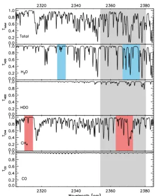
In Fig. 1 we show a simulated transmission spectrum for the entire TROPOMI SWIR spectral range (2305–2385 nm). The top panel shows the total transmission, while the lower four panels show the individual transmissions of the main
Figure 1.Simulated spectral transmittance in the SWIR spectral range, showing the total transmittance (top panel) as well as the ab-sorption features of the individual species (lower four panels). The simulation was performed assuming a solar zenith angle of 0◦and a
viewing zenith angle of 40◦. The 2354.0–2380.5 nm retrieval
win-dow is indicated in grey. The coloured winwin-dows highlight the weak and strong absorption bands of H2O (blue) and CH4(red) used for cloud filtering.
absorbing species (H2O, HDO, CH4 and CO). For the re-trieval of the HDO and H2O total column densities we chose the spectral window between 2354.0 and 2380.5 nm (indi-cated with the grey band), as a trade-off between inclusion of the strongest HDO absorption lines with only minor overlap with the strongest H2O absorption lines. The smaller spec-tral windows in blue (H2O) and red (CH4) indicate the weak and strong absorption bands used for cloud filtering (see be-low). Although we additionally fit H182 O to improve the fit quality of the other species, its absorption lines are weaker than those of HDO (not shown). An accurate retrieval of to-tal column H18
2 O in this spectral range is not yet feasible and therefore not part of the final retrieval product.
For the following analysis, we define two relative profiles: ρkrel=ρk
ck
(5) and
ρk,krel′= ρk′
ρk
whereρkrelis the relative profile of absorberkwith respect to the vertically integrated total column
ck=
Z
ρk(z)dz , (7)
and ρk,krel′ is the relative profile of absorberk′ with respect to absorber k. Assuming that the abundance of trace gask changes by a scaling of the reference profileρkrel, the deriva-tive of the total optical depth with respect to the trace gas column density is given by
∂τtot ∂ck
= 1 ck
Z
σk(z, λ) ρk(z)dz, (8)
thus ∂ITOA
∂ck
= −I TOA
e µck
Z
σk(z)ρk(z)dz . (9)
Corresponding expressions hold for the radiance derivative with respect to the trace gas concentration at a certain altitude level. Finally, the derivative ofITOAwith respect to surface albedoAsis
∂ITOA ∂As =
µ0F0
π exp
−1
e µτtot
. (10)
After the spectral convolution in Eq. (1), we have a linearized forward model:
F(x,b)=F(x0,b)+K{x−x0} +O(x2), (11) with de Jacobian K=∂∂Fx(x0,b). Here, we distinguish be-tween the state vector x that comprises in its components the parameters to be retrieved and forward model parame-tersbdescribing parameters other than the state vector that
influence the measurement. Equation (11) represents a Tay-lor expansion of the forward model around state vectorx0 truncated to first order.
2.2 Inversion
To determine the column density of water vapour isotopo-logues from SWIR measurements, we adjust the state vec-tor x to fit the forward model to the measurement vector y, with spectral residuals ey, by a least squares fitting
ap-proach. The state vectorxincludes the total columns of CO,
CH4, H2O, H18
2 O and HDO, two coefficients to describe the linear spectral dependence of the surface albedo As, and a spectral shift of the ISRF to adjust the spectral calibration of the TROPOMI instrument per retrieval. We apply the profile scaling approach as described by Borsdorff et al. (2014) em-ploying a Gauss–Newton iteration scheme. The least squares minimization problem
ˆ
x=min
x ||S
−1/2
y (F(x)−y)||2 (12)
is solved per iteration step with the solution ˆ
x =x0+G(y−F(x0)), (13)
with the gain matrix
G=(KTS−1y K)−1KTS−1y (14)
and the measurement covariance matrixSy.
After convergence, the column averaging kernel can be calculated in a straightforward manner:
Ak,k′ =
dcret,k
dρk′
=gkK
prof
k′ . (15)
gk is the row vector of the gain matrix G that belongs to
the trace gaskandKprofk′ is the forward model Jacobian with respect to the trace gas profileρk′. The height dependence of the profileρk′ is omitted for a clear presentation. For the full mathematical proof, the reader is referred to Borsdorff et al. (2014). Fork6=k′,Ak,k′ describes the interference of the retrieved columnckwith the real trace gas vertical
distri-bution of another trace gask′. Fork=k′, it is the standard column averaging kernel and we use the more simple nota-tionAk=Ak,k.
The relation between our retrieval productcret,k (the
re-trieved total column of speciesk) and the true state (concen-tration profileρk) of the atmosphere is given by
cret,k=Akρk+
X
k′6=k
Ak,k′ρk′+ex, (16)
whereex is the error on the retrieved total column due to
the forward model and measurement errorsey. In the case
of a single trace gas retrieval the interference termsAk,k′ do
not exist. In such case, the meaning of the remaining col-umn averaging kernelAk is related to the proper choice of
the reference profile and the effective null space of the reg-ularization (see the discussion in Borsdorff et al., 2014 and Wassmann et al., 2015). If the chosen reference profile is cor-rect, the equation is equal to a geometrical integration ofρk.
In the case of multiple trace gas retrievals, we need to assess Eq. (16) in more detail. Using Eq. (6), the above equation can be written as
cret,k=
Ak+
X
k′6=k
ρk,krel′Ak,k′
ρk+ex, (17)
showing that the contribution of the interference kernelAk,k′ can be interpreted as an error term for every level of the av-eraging kernelAk. Because atmospheric humidity can show
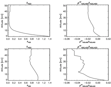
Figure 2.Top left: total column averaging kernel for H2O. Lower
left: total column averaging kernel for HDO. Top right: the sensitiv-ity of total column H2O to variations in HDO at different altitudes. Lower right: the sensitivity of total column HDO to variations in H2O at different altitudes.
by variations in HDO and not a result of the interferences between H2O and HDO. Therefore, we need to test if the in-terferences are small for the casesk=H2O and k′=HDO and vice versa.
Figure 2 shows an example of the column averaging ker-nelsAH2OandAHDO, including the interference kernels mul-tiplied with the relative profiles as in Eq. (17). The averaging kernel for H2O (AH2O, top left panel) shows that the retrieval is only sensitive to H2O in the lower atmosphere. This is a result of strong pressure broadening of the H2O absorp-tion lines (Frankenberg et al., 2009). Since the HDO lines are weaker, the averaging kernel for HDO (AHDO, lower left panel) is more uniform, showing only slightly lower sensitiv-ity at high layers. The interference kernels show that above ∼10 km variations of HDO have a minor impact on the retrieval of H2O (ρrelH2O,HDOAH2O,HDO ≈ −0.02, top right panel in Fig. 2), and variations of H2O have a small impact on the retrieval of HDO (ρrelHDO,H2OAHDO,H2O ≈ −0.04±0.01,
lower right panel in Fig. 2). Since the column averaging ker-nelsAH2O andAHDOare much larger, and the density pro-files ρH2O andρHDO will be very low higher in the atmo-sphere, the induced errors on the total columns due to this interference are practically negligible.
For a proper error characterization of the retrieval product, we calculate the error covariance matrixSxby
Sx=GSyGT . (18)
This allows us to quantify the retrieval noise standard devi-ation σk of the individual column densities and a possible
correlation between them.
For data interpretation, it is common to consider the relative abundance of HDO with respect to H2O: r = cret,HDO/cret,H2O, and to reference the ratio to the Vienna Standard Mean Ocean Water (VSMOW) ratio rs = 3.1153×10⁻⁴:
δD= r
rs−1
, (19)
whereδD is typically given in units of per mil. The first stud-ies that measuredδD in the atmosphere (as mentioned in the introduction) have shown that typical variations inδD over time or space are of the order of 50–100 ‰, which we there-fore regard as the required accuracy for a useful product. The diagnostic tools of the individual columns can be used to de-rive the corresponding quantities for δD. For example, the standard deviation of the retrieval noise is given by
σδD= r rs
v u u tσH2O2
c2H2O + σHDO2
cHDO2 −
2SHDO,H2O
cH2OcHDO, (20)
and in a similar manner the column averaging kernel with respect to the H2O and HDO abundance can be derived.
2.3 Two-band cloud filtering
Since the HDO and H2O retrieval algorithm does not account for clouds nor any other scattering layers, we need to filter for clouds to avoid large retrieval inaccuracies. This filter-ing is achieved usfilter-ing the retrieved columns in a weak and strong absorption band of either CH4 or H2O. The bands used are indicated in Fig. 1. Elevated scattering layers not ac-counted for in the forward model generally cause a retrieval bias by scattering photons directly into the instrument. This optical path length shortening leads to negative biases in the retrieved total columns. The 2-band cloud filter relies on the fact that a total column measurement using a strong absorp-tion band is more strongly affected by this “shielding bias” than the measurement using a weak absorption band. As a result, the relative difference in the retrieved total column between the weak and strong absorption band can be used to indicate the presence of clouds. Using a set of simulated mea-surements for varying cloudy conditions (as will be described in Sect. 3.1), we have tested that using a threshold<6 % for the relative difference in total column CH4between the weak and strong bands we filter for ground scenes that have a cloud fraction of more than 10–20 % (cloud top height ≥1 km). Scenes with low-level clouds (cloud top heights<1 km) are not affected by this filter. Since low-level clouds above sea pass the filter, the retrieval allows for measurements over sea above these clouds due to their high albedo. The albedo of the sea surface itself is too low in the shortwave infrared for a meaningful retrieval above cloud-free sea pixels.
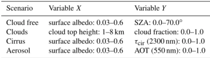
Table 1. Overview of the generic scenarios used for the perfor-mance analysis. For the scenarios where the SZA was not variable, it was fixed at 50◦. For the clouds scenario the surface albedo was
fixed at 0.05.
Scenario VariableX VariableY
Cloud free surface albedo: 0.03–0.6 SZA: 0.0–70.0◦ Clouds cloud top height: 1–8 km cloud fraction: 0.0–1.0 Cirrus surface albedo: 0.03–0.6 τcir(2300 nm): 0.0–1.0
Aerosol surface albedo: 0.03–0.6 AOT (550 nm): 0.0–1.0
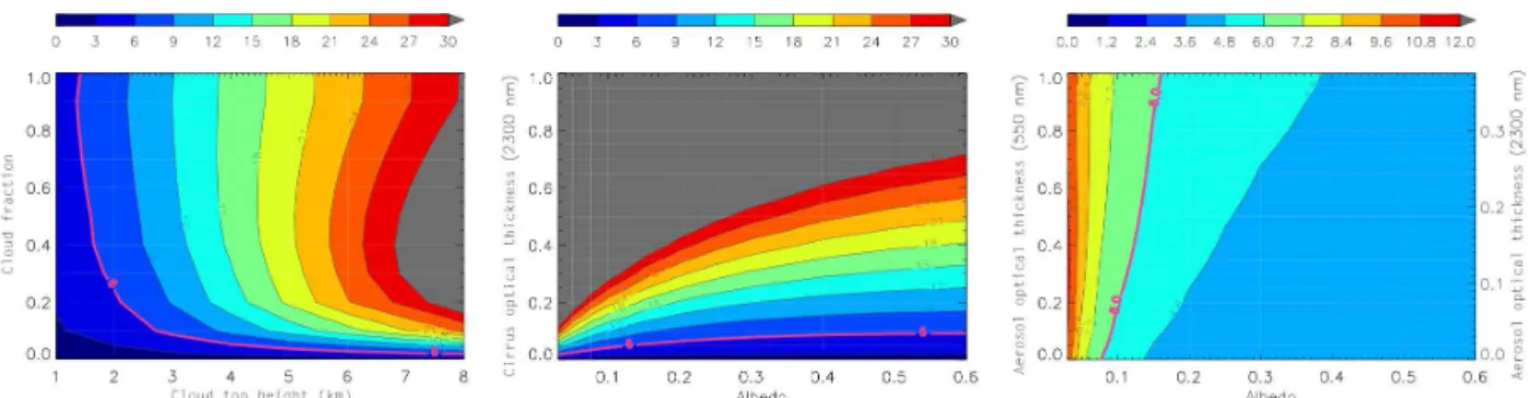
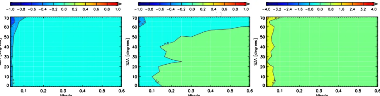
absorption bands (shown in red in Fig. 1) changes for the scenarios with clouds (left panel), cirrus (middle panel) and aerosol (right panel). Scenes with strongest effects on the light path of the observed signal will also show the largest relative difference. We find that with a relative difference in methane absorption <6 % (indicated with the pink curve) we effectively filter for clouds and cirrus, as well as for low surface albedo scenes affected by aerosol. For example, not affected by the filter are scenes with a cloud top height.1 km or scenes with a low fraction of higher-level clouds (i.e. ev-erything below or left of the pink curve in the left panel of Fig. 3). A similar performance is achieved with a 2-band wa-ter filwa-ter, using the weak and strong wawa-ter bands as shown in blue in Fig. 1 and a threshold for the relative difference in water absorption in these bands of 8 %. In the next sections the impact of this cloud filter on the retrievals of HDO and H2O will be shown.
The 2-band cloud filtering will be part of TROPOMI’s op-erational methane preprocessing pipeline (Hu et al., 2016), so synergies with the operational data processing can be used to reduce the processing time significantly, as we have es-timated that on average 20 % of all the measured ground scenes will pass the cloud filter above land, and 14 % above sea.
3 Performance analysis for generic scenarios
To assess the performance of the retrieval algorithm, we ap-plied the retrieval to simulated measurements for various generic scenarios. For each scenario, we systematically var-ied two variables such as surface albedo, solar zenith angle (SZA), cloud parameters (cloud top height, cloud fraction and cloud optical thickness (τcld)) and aerosol optical thick-ness (AOT). An overview of the scenarios is given in Table 1.
3.1 Measurement simulations
The measurement simulations for the generic scenarios were created using the S-LINTRAN radiative transfer model (Schepers et al., 2014). The implementation of S-LINTRAN for TROPOMI simulations, including the instrument model, is described in detail in Landgraf et al. (2016), as the same simulations have been used to assess the performance of the
Table 2.Microphysical properties of water and ice clouds:n(r) rep-resents the size distribution type,reffandveffare the effective radius
and variance of the size distribution,m=n−ikis the refractive
in-dex. The ice cloud size distribution follows a power-law distribution as proposed by Heymsfield and Platt (1984).
Water clouds Ice clouds
n(r) gamma (r/ri)−3.85
reff[µm] 20 – veff 0.10 –
n 1.28 1.26
k 4.7×10⁻⁴ 2.87×10⁻⁴
CO retrieval algorithm. A summary of the implementation is provided in the following two paragraphs.
The model is a scalar plane–parallel radiative transfer model that fully accounts for multiple elastic light scatter-ing by clouds, cirrus, air molecules and the reflection of light from the Earth’s surface. The optical properties of wa-ter clouds are calculated using Mie theory with microphysi-cal cloud properties given in Table 2. For ice clouds the ray-tracing model of Hess and Wiegner (1994); Hess et al. (1998) is employed assuming hexagonal, columnar ice crystals ran-domly oriented in space. Cirrus and water clouds are de-scribed by cloud top and base height, and cloud optical thick-ness. While cirrus fully cover the observed ground scene, wa-ter clouds can show partial cloud coverage by utilizing the independent pixel approximation (Marshak et al., 1995) for the simulation.
Measurement noise was superimposed on the radiance spectra using the TROPOMI noise model (Tol et al., 2011). This assumed an observed ground scene of 7×7 km2 and a telescope aperture of 6×10⁻⁶m2. The resulting signal-to-noise ratio is 120 in the continuum of the spectrum for a dark reference scene (surface albedoAs=0.05, viewing zenith angle VZA=0◦and solar zenith angle SZA=70◦).
The atmospheric model assumed the US standard atmo-sphere (1976) for the profiles of dry air density, temperature, pressure, water and CO. The CH4 profile is taken from the CAMELOT European background profile scenario (Levelt and Veefkind, 2009), interpolated to the same pressure grid and converted from mixing ratios to densities using the air densities from the US standard atmosphere. We separated the water profile into individual profiles for the three iso-topic components with absorption features in the TROPOMI SWIR range: H16
2 O, H182 O and HDO. First, the water pro-file was scaled with the VSMOW abundance of the respec-tive species. Additionally, a realistic altitudependent de-pletion of HDO and H18
Figure 3.2-Band CH4filter results for clouds (left), cirrus (middle) and aerosol (right). Plotted is the relative difference in total column
CH4retrieved from the weak and strong bands: CH4(weak – strong)/strong ( %). The cloud scenario assumed a cloud optical thickness ofτcld=5 and a variable cloud-top-height (xaxis) and cloud fraction (yaxis). The cirrus scenario assumed a cloud fraction of 100 % for a layer between 9 and 10 km and a variable surface albedo (xaxis) and cirrus optical thickness (yaxis). The aerosol scenario assumed a
sulphate-type aerosol in the boundary layer between 0 and 2 km, a variable surface albedo (xaxis) and aerosol optical thickness (yaxis). The
pink curve shows the 6 % threshold that will be used for filtering.
Figure 4.Atmospheric profiles for the number densities of the
ab-sorbers (bottom axis, normalized to the surface value) and temper-ature (top axis) used as input for the model atmosphere.
2010). We further assumed that the concentration of H182 O is related to the concentration of HDO according to the empir-ically determined “global meteoric water line” (Craig, 1961)
δD=8·δ18O+10 ‰, (21)
whereδ18O is defined in the same way asδD (Eq. 19). All the atmospheric profiles used for the measurement simulations are shown in Fig. 4.
In the following subsections, we characterize the retrieval performance for the generic scenarios, separately consider-ing the retrieval statistical errors (i.e. the sconsider-ingle-measurement noise), σH2O, σHDO and σδD (neglecting the small HDO– H2O cross-correlation term forσδD), and the biases in the
total columns cret,H2O,cret,HDO and their ratioδD. The
re-trieval statistical error estimate forδD is given by Eq. (20). For the bias in δD, which we refer to as “1δD”, we first
determineδDretrieval by removing the noise on the retrieved total columns HDO and H16
2 O using linear error propaga-tion for the particular noise realizapropaga-tion. We need to compare δDretrieval withδDmodel, whereδDmodel isδD of the “true” model atmosphere:
δDmodel=ctrue,HDO ctrue,H2O
1
rs−1 . (22)
Finally, the retrieval bias onδD is defined as
1δD=δDretrieval−δDmodel. (23) 3.2 Cloud-free conditions
In Fig. 5 we show the simulated cloud-free retrieval bias for the total column H2O (left panel), total column HDO (mid-dle panel) and their ratio (1δD, right panel) as a function of surface albedo and SZA (no clouds or aerosol present). The figure shows that the retrieval performs very well for the ma-jority of the scenes, with1δD less than 0.8 ‰. Only for the lowest surface albedos (0.03–0.05) the bias inδD increases to a few per mil, due to slightly more negative bias in H2O compared to HDO.
3.3 Clouds and cirrus
As the retrieval algorithm does not account for scattering, any clouds, cirrus and aerosol present in the observed scene will lead to biases in the retrieval of the total columns HDO and H2O. We have tested the performance of the retrieval under cloudy conditions with a scenario assuming a cloud with an optical thickness ofτcld=5, with varying cloud top heights (between 1 and 8 km in steps of 1 km) and varying cloud fractions (between 0.0 and 1.0 in steps of 0.1). The same scenario was used to demonstrate the 2-band cloud filter in the left panel of Fig. 3. Due to differences in their retrieval sensitivities, the observed bias is stronger for H2O than for HDO, leading to significant biases in their ratio, increas-ing with both cloud fraction and cloud top height (although not shown, we find that1δD can reach values>900 ‰ for clouds above 7 km with 100 % cloud coverage). Similarly, by simulating scenarios with varying surface albedos and a uni-form cirrus or aerosol layer with varying optical thickness (see Table 1), we find that this bias increases with the op-tical thickness of the layer and with lower surface albedos, as both lead to a lower contribution of photons from below the scattering layer reaching the instrument. As described in Sect. 2.3, the 2-band cloud filtering technique will be used to prefilter the scenes most affected by this shielding bias. We find that, after applying the 2-band methane filter to scenes affected by clouds and cirrus, 1δD.70 ‰ andσδD=10– 20 ‰ (for scenes with a low surface albedo ofAs=0.05). 3.4 Aerosol
An aerosol layer typically has a lower optical thickness than clouds and occurs lower in the atmosphere, leading to a dif-ferent impact on our non-scattering retrieval. Our aerosol scenario assumes a uniform layer of a sulphate-type aerosol in the boundary layer between 0 and 2 km. Figure 7 shows how this induces a bias in the total columns H2O, HDO and their ratio, as a function of aerosol optical thickness and sur-face albedo. We see that for very low sursur-face albedos, direct reflection off the aerosol layer leads to path length shorten-ing and a correspondshorten-ing negative (shieldshorten-ing) bias for the total column H2O. This effect is weaker for HDO due its more uni-form averaging kernel. For higher surface albedos, however, we see that the bias becomes positive, likely due to an in-creased amount of light scattering in the boundary layer. The contribution of photons from the brighter surface increases and a fraction of these photons undergo multiple scattering events between the aerosol layer and the surface, enhancing the path length. The net effect onδD is that its bias due to aerosol is highest for the lowest surface albedos and highest AOT (right panel in Fig. 7). If we take the 2-band cloud filter into account (the pink curve coming from Fig. 3) to filter the lowest surface albedos affected by aerosol, we are left with 1δD.20 ‰ due to boundary layer aerosol with AOT=1.0 (at 550 nm). The statistical error (not shown) does not
de-pend significantly on AOT, but varies primarily with surface albedo, reaching similar peak values as in the cloud-free sce-nario (σδD≈20 ‰).
3.5 Summary of the general performance
In summary, we can conclude that the retrieval performs well under cloud-free conditions. The bias1δD will be less than 2 ‰, even for the lowest surface albedos, and the statisti-cal errors vary from 2–4 ‰ for high albedos to 15–25 ‰ for the lowest albedos. Under conditions with clouds, cirrus or aerosol the retrieval performs less well and we generally find a positive bias inδD. To restrict this bias we need strict filter-ing against clouds and aerosol by applyfilter-ing the 2-band cloud filter either to methane or water (which additionally leads to a great reduction in the computational effort). Applying a 2-band methane threshold of 6 %, we restrict the bias inδD to1δD < 70 ‰ for all simulated measurements. Averag-ing multiple sAverag-ingle measurements over time and space will further reduce the statistical error and will improve the accu-racy to better than the maximum 70 ‰. This brings the mea-surements within the minimum requirement to study, e.g. the range of seasonality and the meridional variation, which are of the order of 50–100 ‰. On smaller temporal and spatial scales, such as local daily variability, a higher accuracy is needed, which TROPOMI is able to deliver as long as the conditions are cloud free and only moderately affected by aerosol.
4 Sensitivity to prior assumptions
Similarly to what was done for the CO TROPOMI retrievals (Landgraf et al., 2016), we have tested the sensitivity of the H2O and HDO total column retrievals to the prior assump-tions, including the impact onδD. These so-called forward modelling errors were tested on the cloud-free scenario (with varying SZA and surface albedo) using the same measure-ment simulation as described in Sect. 3. A perturbation in one of the input assumptions was introduced, after which the retrievals were performed and compared with the default re-trievals without the perturbation. The impact of the perturba-tion is expressed as a systematic error and standard deviaperturba-tion, where we define the systematic error as the mean difference inδD between the perturbed and default retrievals for the 45 scenes with the three lowest surface albedos (0.03, 0.05 and 0.075). The results are summarized in Table 3.
Figure 5.Cloud-free retrieval bias as a function of surface albedo and SZA for the total columns of H2O (left, %), HDO (middle, %) and
the HDO/H2O ratio (right, ‰).
Figure 6.Cloud-free statistical error estimates (single-measurement noise) as a function of surface albedo and SZA for the total columns of H2O (left, %), HDO (middle, %) and the HDO/H2O ratio (right, ‰).
Table 3.Summary of the sensitivity to the meteorological input and instrument parameters, expressed as the mean difference inδD
be-tween the perturbed and default retrievals for the 45 scenes with the three lowest surface albedos (0.03, 0.05 and 0.075).
Prior parameter Systematic error inδD [‰]
Temp−0.5 K −6.9±0.74
Temp+0.5 K +7.0±0.11
Temp−1 K −14±0.74
Temp+1 K +14±0.17
Pressure×0.99 −4.5±0.74
Pressure×1.01 +4.5±0.54
Rad. offset+0.1 % −0.054±0.11
Rad. offset+0.5 % −0.20±0.16
ISRF FWHM−1 % +0.36±0.85
ISRF FWHM+1 % −0.33±0.84
This error is constant for all surface albedos and SZAs and scales linearly with the size of the temperature perturbation.
The atmospheric pressure profile is derived from the sur-face pressure. To test the impact on inaccuracies in the ECMWF surface pressure, we applied a perturbation of ±1 %. This leads to systematic errors of about 0.5 % in H2O and 0.13 % in HDO (with reversed sign), together inducing errors of about 4.5 ‰ inδD.
The retrieval algorithm requires a reflectance spectrum, acquired by dividing the radiance spectrum measured from the Earth’s surface by the irradiance spectrum measured directly from the Sun. Differences in the radiometric off-set between these spectra could induce spectral features in the reflectance spectrum, leading to systematic errors. The TROPOMI instrument requirement for the radiometric off-set on the radiance is 0.1 % of the continuum level. We have tested the impact of an offset on the radiance of 0.1 and 0.5 % of the maximum value in the retrieval window. However, the retrieval fits for an offset in the reflectance spectra, which partly mitigates the effects of an offset in the radiance or ir-radiance. The systematic errors due to uncertainties in the radiometric offset are therefore very small (errors inδD less than 0.5 ‰).
For the default retrieval and measurement simulations we have assumed a Gaussian slit function (ISRF) with a full width at half maximum (FWHM) of 0.25 nm. We have tested the impact of perturbing this FWHM by±1 % and find that the induced systematic errors are strongly dependent on sur-face albedo and SZA. The largest errors inδD reach±3 ‰ and are found for high albedos and low SZAs. The mean sys-tematic error for the lowest albedos is 0.36±0.85 ‰.
Figure 7.Retrieval bias for an aerosol layer between 0 and 2 km as a function of surface albedo and AOT for the total columns of H2O
(left, %), HDO (middle, %) and the HDO/H2O ratio (right, ‰). The pink curve shows the 6 % methane cloud filter threshold from Fig. 3.
Applying that filter would result in filtering of the scenes left of the pink line.
profiles are expected to be mostly quasi-random in nature, which means their impact on the error inδD will diminish when taking averages in time and space.
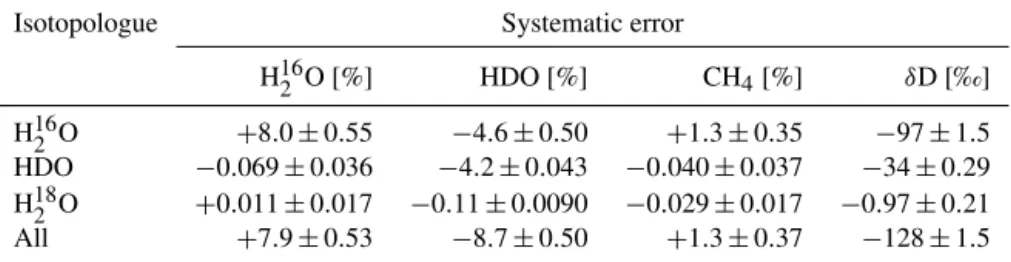
More structural systematic errors (i.e. those that will not diminish by averaging) are potentially caused by uncertain-ties in the water spectroscopy. Recent studies have shown that spectroscopic uncertainties of water can have a large im-pact on total column retrievals of CO (Galli et al., 2012), CH4(Frankenberg et al., 2008; Schneising et al., 2009), H2O (Schrijver et al., 2009) and the HDO/H2O ratio (Scheep-maker et al., 2013). As a test of the possible impact of uncer-tainties in the water line parameters, we have repeated the re-trievals of the simulated clear-sky scenario after replacing the line parameters of the water isotopologues. For the simulated spectra the parameters from the high-resolution transmission database were used (HITRAN, Rothman et al., 2009). We then performed the retrievals using the water line parame-ters from Scheepmaker et al. (2013). Table 4 shows the in-duced systematic errors for replacing a single isotopologue at a time, and for replacing all modelled water isotopologues simultaneously. It shows that the retrieval of HDO and H2O can be very sensitive to spectroscopic uncertainties, espe-cially for the ratio HDO/H2O, since HDO and H162 O can show sensitivities with opposite sign, which strengthen each other when taking the ratio (as can be seen from replacing only the H16
2 O parameters). The differences in spectroscopy between HITRAN and Scheepmaker et al. (2013) can lead to differences inδD of up to 128 ‰. Although we find that the differences do not depend on surface albedo or SZA, we cannot exclude a dependency on the total amount of wa-ter vapour, which might lead to seasonal and latitudinal bi-ases. Similar to the retrieval of CO (Galli et al., 2012), the HDO/H2O retrieval will very likely benefit from a reassess-ment of the spectroscopic line parameters of water, a study which is currently ongoing (Loos et al., 2015). Regardless of such reassessments, validation studies will be needed to ver-ify spectroscopy and to define corrections that might mitigate spectroscopy related biases.
5 Performance analysis for a realistic scenario
To show the capabilities of the TROPOMI H2O and HDO total column retrievals, we have simulated an ensemble of measurements that reflect a realistic scenario as accurately as possible. In Sect. 5.1 we describe the input data and mea-surement simulations in more detail. In Sect. 5.2 we discuss the results of retrieving the simulated measurements in terms of retrieval bias, precision, and effectiveness of the cloud fil-tering.
5.1 Measurement simulations
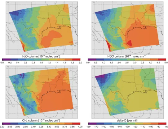
The simulated measurement ensemble covers a region over the south-western US and north-eastern Mexico as observed by TROPOMI on 4 August 2009. Figures 8 and 9 show the region in terms of various input fields. This region comprises a clear gradient in the relative abundance of HDO with re-spect to H2O due to the transport of humid air from coastal regions inland. We have combined data from the MODIS Aqua satellite (clouds, land/water coverage, surface albedo, aerosol) with data from ETOPO5 (elevation), ECMWF (sur-face pressure, temperature profiles, specific humidity), TM5 (CO and CH4 profiles) and LMDZiso (HDO and H182 O profiles) to simulate 27405 TROPOMI measurements on a grid of 135 by 203 ground pixels. This ensemble represents roughly what TROPOMI will observe in 5 min with a daily revisiting cycle.
pix-Table 4.Sensitivity to a change of water line parameters from HITRAN2008 to the parameters from Scheepmaker et al. (2013).
Isotopologue Systematic error
H162 O [%] HDO [%] CH4[%] δD [‰]
H162 O +8.0±0.55 −4.6±0.50 +1.3±0.35 −97±1.5 HDO −0.069±0.036 −4.2±0.043 −0.040±0.037 −34±0.29
H182 O +0.011±0.017 −0.11±0.0090 −0.029±0.017 −0.97±0.21
All +7.9±0.53 −8.7±0.50 +1.3±0.37 −128±1.5
els. Only clouds with top height above 100 m were used. We derived cirrus optical thicknesses from the MODIS cirrus re-flectance product employing the algorithm by Dessler and Yang (2003). For all pixels, the cirrus was located between 9 and 10 km. For the aerosol optical thickness (at 550 nm) we used the MODIS MYD08_M3 global monthly mean product (Platnick et al., 2015b), resampled to the above-mentioned granule with a pixel size of 10×10 km2at subsatellite point. For some pixels with missing aerosol data the optical thick-ness was set to 0.1. We assumed three different aerosol types: oceanic (above water), dust (above land), and urban (above all land regions with AOT>0.23). The corresponding model fields are depicted in Fig. 8.
The distribution of atmospheric trace gases was estimated using TM5 chemistry model simulations (Krol et al., 2005), which yields the CO and CH4 abundances. Moreover, we used data from ECMWF (Dee et al., 2011) for the at-mospheric pressure, temperature and humidity profiles. For realistic HDO/H2O ratios we derived δD profiles from LMDZiso model simulations (Risi et al., 2010) and for the δ18O profiles we assumed correlation toδD according the global meteoric water line (also see Eq. (21), Craig, 1961). Figure 9 shows the resulting total columns for the most im-portant species for our ensemble. Based on this input and the TROPOMI instrument model as described in Sect. 3.1, we simulated for each individual pixel the TROPOMI SWIR ob-servations using the S-LINTRAN radiative transfer model.
5.2 Results
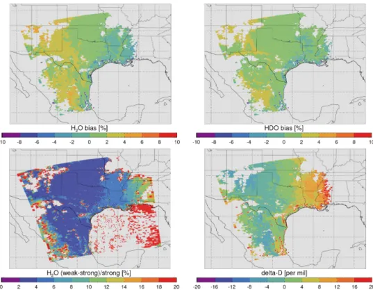
Using the simulated measurement ensemble we retrieved the water vapour abundances using the SICOR retrieval algo-rithm including the retrieval of the two methane and water bands used for cloud filtering. In Fig. 10 the results are shown in terms of the retrieved bias in total column H2O, HDO and δD. We also show the relative difference in the weak vs. strong water bands that were used for cloud filtering. The cloud filter panel (lower left panel in Fig. 10) shows that the algorithm retrieved some pixels above the Gulf of Mexico, even though these pixels did not contain low-level clouds. In reality such pixels will be removed by prefiltering for very low albedo regions. Once the 2-band cloud filter threshold is applied (keeping only pixels with a relative difference<8 % using the water bands), practically all ocean pixels are
moved, as well as all the lands pixels affected by clouds, re-sulting in 54.5 % of the pixels remaining for further study. Using the two methane bands as a cloud filter with a thresh-old of 6 % resulted in slightly less strict filtering (60.7 % of the pixels remaining), as certain pixels with low and optical thin clouds in the west above Mexico and in the east above Alabama were not removed (not shown). The few rejected pixels in the centre and south of Texas show that the cloud filter effectively removed high isolated clouds with low opti-cal thickness (cf. the lower two panels in Fig. 8 with Fig. 10), but left pixels with clouds<1 km intact (as is preferred). The large group of pixels in the north-east of the ensemble were rejected based on the presence of high and optically thick clouds, or the presence of aerosol above low surface albedo regions.
Figure 8.A selection of the input for the realistic scenario simulation. Top left: SWIR surface albedo. Top right: aerosol optical thickness at 550 nm. Bottom left: cloud optical thickness. Bottom right: cloud top height.
Figure 9.Input total columns for the most important absorbing species for the realistic scenario simulation. Top left: H2O. Top right: HDO.
Figure 10.Retrieval biases for water in the realistic scenario simulation. Except for the bottom left panel, the results are cloud filtered using a weak vs. strong water band threshold of 8 %. Top left: H2O bias. Top right: HDO bias. Bottom left: relative difference in the weak vs. strong water bands used for cloud filtering. Bottom right: bias in the derived HDO/H2O ratio.
Figure 11.Retrieved, cloud-filtered, single-measurement precision of H2O (top left), HDO (top right), CH4(bottom left) and of the derived
elevated (or drier) areas and lower elevated (or more humid) areas.
Figure 11 shows the same maps in terms of single-measurement precision error (1σ). As expected, the domi-nant factor to determine the precision error is surface albedo. The error of the strong absorbers H2O and CH4 is 0.05– 0.15 % for the highest surface albedos, which increases to 0.35 % for the lowest surface albedos. The precision errors of the weak absorber HDO are larger, reaching 0.50 % for the lowest surface albedos. This translates into precision er-rors inδD of at most 5 ‰ above the lowest albedos.
This realistic scenario demonstrates the capabilities of TROPOMI and the SICOR algorithm to retrieve accurate pat-terns in total column H2O, HDO andδD above land from a single overpass. After the 2-band cloud filter effectively removed all measurements above water and high clouds, a small bias remains due to aerosol, which correlates with sur-face albedo. The bias is smaller (and of opposite sign) com-pared to the temporal or spatial gradients inδD expected for typical science cases (e.g. as observed by SCIAMACHY in Yoshimura et al., 2011; Lee et al., 2012; Risi et al., 2012a; Okazaki et al., 2015). This ensures the ability to detect and study patterns in δD on much smaller timescales and at higher spatial resolution compared to previous satellite mis-sions, but care should be taken when using the data over re-gions with strong gradients in surface albedo.
6 Discussion and conclusions
We have presented an algorithm and performance analy-sis for the retrieval of total column H2O and HDO from TROPOMI measurements onboard the Sentinel-5 Precur-sor mission. By adapting ESA’s operational CO algorithm (Landgraf et al., 2016), we developed a relatively simple ap-proach that is fast but relies on strict filtering for clouds, cir-rus and aerosol using a 2-band methane or water retrieval. The ratio HDO/H2O will be a useful scientific product in the fields of hydrology and climate research, with the poten-tial to improve our understanding of the processes controlling atmospheric humidity and transport.
The first studies in this direction which used a similar type of column-averaged satellite product were using SCIA-MACHY data (Frankenberg et al., 2009; Yoshimura et al., 2011; Lee et al., 2012; Risi et al., 2012b, a; Scheepmaker et al., 2015). These studies showed that the typical seasonal or spatial gradients in δD are about 50–100 ‰. The mea-surement precision and accuracy needs to be higher than this in order to contribute significantly to science. For SCIA-MACHY, this implied either taking monthly averages or bin-ning to a spatial resolution of at least 1×1◦ in order to bring the statistical error down to about 20 ‰ (the single-measurement precision being∼115 ‰, Scheepmaker et al., 2015). The newer GOSAT measurements show an improve-ment in precision by a factor of about 2, compared to
SCIA-MACHY (Frankenberg et al., 2013; Boesch et al., 2013). Both SCIAMACHY and GOSAT products show a negative bias of about 30–70 ‰ compared to ground-based Fourier-transform spectroscopy (FTS) networks.
Our analysis has shown that TROPOMI is expected to deliver a much better performance than SCIAMACHY and GOSAT in terms ofδD in only a single overpass. The single-measurement noise will be better than 15–25 ‰ for even the lowest surface albedos, while at the same time the spatial resolution of 7×7 km2is much higher than SCIAMACHY’s 120×30 km2and provides a better coverage than GOSAT’s sparse spatial sampling. Even though we still need to filter for clouds, due to this higher spatial resolution TROPOMI will observe many more useful scenes in between clouds compared to SCIAMACHY or GOSAT. This allows for new opportunities to study the hydrological cycle on timescales of mere days or weeks instead of seasons or years, or over longer periods if a high spatial resolution is desired.
Mainly due to the presence of low-level aerosol in the at-mosphere, the cloud-filtered TROPOMI measurements of to-tal column HDO and H2O are not expected to be completely bias free. Changes to the light paths of the reflected photons due to any scattering particles remaining after filtering are not accounted for in the retrieval algorithm, and lead to bi-ases of a few percent in total column HDO and H2O, and up to∼20 ‰ inδD, depending on surface albedo, as shown by our simulated scenario of measurements above the USA and Mexico.
After launch and commissioning of the instrument in Q4 2016, validation using ground-based FTS data from the TC-CON and NDACC networks is needed to test the perfor-mance of the algorithm on real measurements. Thermal in-frared products, such asδD from TES and IASI, also provide useful complementary information due to their different sen-sitivity. Therefore, aircraft validation may also be valuable, as in situ measurements could be useful to address any dif-ferences between total column and thermal infrared products. Ideally, the HDO/H2O products from the ground-based net-works should first be intercompared, both using the results from the ongoing reassessment of the water spectroscopy (Loos et al., 2015), and for a range of atmospheric conditions and geographical locations. Any possible differences due to either spectroscopy or location (e.g. as found by Scheep-maker et al., 2015) need to be understood before the next generation of HDO and H2O global retrievals from space can be exploited to come to a better understanding of the atmo-spheric hydrological cycle and the role it plays in our chang-ing climate.
7 Data availability
(j.landgraf@sron.nl). MODIS Aqua MYD06_L2 (Platnick et al., 2015a) and MYD08_M3 (Platnick et al., 2015b) data are available through NASA’s Level 1 and Atmosphere Archive and Distribution System (LAADS, https://ladsweb. nascom.nasa.gov/data/search.html). MODIS MCD43C4 data (Strahler et al., 1999) are available through NASA’s Re-verb tool (http://reRe-verb.echo.nasa.gov/reRe-verb). ETOPO5 data (NOAA, 1988) are available through NOAA (http://www. ngdc.noaa.gov/mgg/global/etopo5.html). HITRAN spectro-scopic line parameters (Rothman et al., 2009) are available through HITRAN Online (http://hitran.org) and the line pa-rameters from Scheepmaker et al. (2013) are available in their Supplement.
Acknowledgements. H. Hu and J. aan de Brugh are in part financed
by the TROPOMI national programme from the Netherlands Space Office (NSO). LMDZiso simulations used the computing resources of IDRIS under the allocation 0292 made by GENCI. We thank the two anonymous referees for their useful comments that improved this paper.
Edited by: B. Veihelmann
Reviewed by: two anonymous referees
References
Aggarwal, P. K., Gat, J. R., and Froehlich, K. F.: Isotopes in the Water Cycle: Past, present and future of a developing science, Springer, Dordrecht, the Netherlands, ISBN-13: 978-1-4020-3023-9, 2005.
Boesch, H., Deutscher, N. M., Warneke, T., Byckling, K., Cogan, A. J., Griffith, D. W. T., Notholt, J., Parker, R. J., and Wang, Z.: HDO/H2O ratio retrievals from GOSAT, Atmos. Meas. Tech., 6,
599–612, doi:10.5194/amt-6-599-2013, 2013.
Borsdorff, T., Hasekamp, O. P., Wassmann, A., and Landgraf, J.: In-sights into Tikhonov regularization: application to trace gas col-umn retrieval and the efficient calculation of total colcol-umn averag-ing kernels, Atmos. Meas. Tech., 7, 523–535, doi:10.5194/amt-7-523-2014, 2014.
Boucher, O., Randall, D., Artaxo, P., Bretherton, C., Feingold, G., Forster, P., Kerminen, V.-M., Kondo, Y., Liao, H., Lohmann, U., Rasch, P., Satheesh, S., Sherwood, S., Stevens, B., and Zhang, X.: Clouds and Aerosols, in: Climate Change 2013: The Physi-cal Science Basis. Contribution of Working Group I to the Fifth Assessment Report of the Intergovernmental Panel on Climate Change, edited by: Stocker, T. F., Qin, D., Plattner, G.-K., Tig-nor, M., Allen, S. K., Boschung, J., Nauels, A., Xia, Y., Bex, V., and Midgley, P. M., Cambridge University Press, Cambridge, United Kingdom and New York, NY, USA, 2013.
Craig, H.: Isotopic Variations in Meteoric Waters, Science, 133, 1702–1703, doi:10.1126/science.133.3465.1702, 1961. Craig, H. and Gordon, L.: Deuterium and oxygen 18 variations in
the ocean and marine atmosphere, in: Stable Isotopes in Oceano-graphic Studies and Paleotemperatures, Spoleto, Italy, edited by: Tongiogi, E., 9–130, V. Lishi e F., Pisa, Italy, 1965.
Dansgaard, W.: Stable isotopes in precipitation, Tellus, 16, 436– 468, 1964.
Dansgaard, W., Johnsen, S. J., Møller, J., and Langway, C. C.: One Thousand Centuries of Climatic Record from Camp Cen-tury on the Greenland Ice Sheet, Science, 166, 377–380, doi:10.1126/science.166.3903.377, 1969.
Dee, D. P., Uppala, S. M., Simmons, A. J., Berrisford, P., Poli, P., Kobayashi, S., Andrae, U., Balmaseda, M. A., Balsamo, G., Bauer, P., Bechtold, P., Beljaars, A. C. M., van de Berg, L., Bid-lot, J., Bormann, N., Delsol, C., Dragani, R., Fuentes, M., Geer, A. J., Haimberger, L., Healy, S. B., Hersbach, H., Hólm, E. V., Isaksen, L., Kållberg, P., Köhler, M., Matricardi, M., McNally, A. P., Monge-Sanz, B. M., Morcrette, J.-J., Park, B.-K., Peubey, C., de Rosnay, P., Tavolato, C., Thépaut, J.-N., and Vitart, F.: The ERA-Interim reanalysis: configuration and performance of the data assimilation system, Q. J. Roy. Meteor. Soc., 137, 553–597, doi:10.1002/qj.828, 2011.
Dessler, A. E. and Yang, P.: The Distribution of Trop-ical Thin Cirrus Clouds Inferred from Terra MODIS
Data, J. Climate, 16, 1241–1247,
doi:10.1175/1520-0442(2003)16<1241:TDOTTC>2.0.CO;2, 2003.
Ehhalt, D. H.: Vertical profiles of HTO, HDO, and H2O in the tro-posphere, NCAR Tech. Note NCAR-TN-STR-100, 1974. Ehhalt, D. H., Rohrer, F., and Fried, A.: Vertical profiles of
HDO/H2O in the troposphere, J. Geophys. Res., 110, 13301, doi:10.1029/2004JD005569, 2005.
Frankenberg, C., Bergamaschi, P., Butz, A., Houweling, S., Meirink, J. F., Notholt, J., Petersen, A. K., Schrijver, H., Warneke, T., and Aben, I.: Tropical methane emissions: A re-vised view from SCIAMACHY onboard ENVISAT, Geophys. Res. Lett., 35, 15811, doi:10.1029/2008GL034300, 2008. Frankenberg, C., Yoshimura, K., Warneke, T., Aben, I., Butz,
A., Deutscher, N., Griffith, D., Hase, F., Notholt, J., Schnei-der, M., Schrijver, H., and Röckmann, T.: Dynamic Pro-cesses Governing Lower-Tropospheric HDO/H2O Ratios as
Ob-served from Space and Ground, Science, 325, 1374–1377, doi:10.1126/science.1173791, 2009.
Frankenberg, C., Wunch, D., Toon, G., Risi, C., Scheepmaker, R., Lee, J.-E., Wennberg, P., and Worden, J.: Water vapor isotopo-logue retrievals from high-resolution GOSAT shortwave infrared spectra, Atmos. Meas. Tech., 6, 263–274, doi:10.5194/amt-6-263-2013, 2013.
Galli, A., Butz, A., Scheepmaker, R. A., Hasekamp, O., Landgraf, J., Tol, P., Wunch, D., Deutscher, N. M., Toon, G. C., Wennberg, P. O., Griffith, D. W. T., and Aben, I.: CH4, CO, and H2O spec-troscopy for the Sentinel-5 Precursor mission: an assessment with the Total Carbon Column Observing Network measure-ments, Atmos. Meas. Tech., 5, 1387–1398, doi:10.5194/amt-5-1387-2012, 2012.
Herbin, H., Hurtmans, D., Clerbaux, C., Clarisse, L., and Co-heur, P.-F.: H162 O and HDO measurements with IASI/MetOp, At-mos. Chem. Phys., 9, 9433–9447, doi:10.5194/acp-9-9433-2009, 2009.
Hess, M. and Wiegner, M.: COP: a data library of optical properties of hexagonal ice crystals, Appl. Opt., 33, 7740–7746, 1994. Hess, M., Koelemeijer, R. B. A., and Stammes, P.: Scattering
matri-ces of imperfect hexagonal ice crystals, J. Quant. Spectrosc. Ra., 60, 301–308, doi:10.1016/S0022-4073(98)00007-7, 1998. Heymsfield, A. J. and Platt, C. M. R.: A
Content., J. Atmos. Sci., 41, 846–855, doi:10.1175/1520-0469(1984)041<0846:APOTPS>2.0.CO;2, 1984.
Hu, H., Hasekamp, O., Butz, A., Galli, A., Landgraf, J., Aan de Brugh, J., Borsdorff, T., Scheepmaker, R., and Aben, I.: The operational methane retrieval algorithm for TROPOMI, At-mos. Meas. Tech. Discuss., doi:10.5194/amt-2016-108, in re-view, 2016.
Jouzel, J., Russell, G. L., Suozzo, R. J., Koster, R. D., White, J. W. C., and Broecker, W. S.: Simulations of the HDO
and H218O atmospheric cycles using the NASA/GISS
general circulation model: The seasonal cycle for present-day conditions, J. Geophys. Res., 92, 14739–14760, doi:10.1029/JD092iD12p14739, 1987.
Jouzel, J., Alley, R. B., Cuffey, K. M., Dansgaard, W., Grootes, P., Hoffmann, G., Johnsen, S. J., Koster, R. D., Peel, D., Shuman, C. A., Stievenard, M., Stuiver, M., and White, J.: Validity of the temperature reconstruction from water isotopes in ice cores, J. Geophys. Res., 102, 26471–26488, doi:10.1029/97JC01283, 1997.
Kasten, F. and Young, T.: Revised optical air mass tables and ap-proximation formula, Appl. Opt., 28, 4735–4738, 1989. Krol, M., Houweling, S., Bregman, B., van den Broek, M., Segers,
A., van Velthoven, P., Peters, W., Dentener, F., and Bergamaschi, P.: The two-way nested global chemistry-transport zoom model TM5: algorithm and applications, Atmos. Chem. Phys., 5, 417– 432, doi:10.5194/acp-5-417-2005, 2005.
Kurylo, M. and Solomon, S.: Network for the Detection of Strato-spheric Change: A Status and Implementation Report, NASA, Upper Atmosphere Research Program and NOAA Climate and Global Change Program, Washington DC, 1990.
Landgraf, J., aan de Brugh, J., Scheepmaker, R., Borsdorff, T., Hu, H., Houweling, S., Butz, A., Aben, I., and Hasekamp, O.: Carbon monoxide total column retrievals from TROPOMI shortwave infrared measurements, Atmos. Meas. Tech. Discuss., doi:10.5194/amt-2016-114, in review, 2016.
Lee, J.-E., Risi, C., Fung, I., Worden, J., Scheepmaker, R. A., Lintner, B., and Frankenberg, C.: Asian monsoon hydrometeo-rology from TES and SCIAMACHY water vapor isotope mea-surements and LMDZ simulations: Implications for speleothem climate record interpretation, J. Geophys. Res., 117, D15112, doi:10.1029/2011JD017133, 2012.
Levelt, P. and Veefkind, P.: ESA CAMELOT study: Challenges in future operational missions for GMES atmospheric monitoring, sentinel 4 and 5, in: EGU General Assembly Conference Ab-stracts, edited by Arabelos, D. N. and Tscherning, C. C., vol. 11 of EGU General Assembly Conference Abstracts, p. 8911, 19– 24 April 2009.
Loos, J., Birk, M., Wagner, G., Mondelain, D., Kassi, S., Vasilchenko, S., Campargue, A., Hase, F., Dufour, G., Eremenko, M., Orphal, J., Cuesta, J., Bigazzi, A., Perrin, A., Daumont, L., and Zehner, C.: Spectroscopic database for TROPOMI/Sentinel-5 Precursor, in: ESA ATMOS 201TROPOMI/Sentinel-5 Conference Proceedings (ESA SP-735), 8–12 June 2015.
Marshak, A., Davis, A., Wiscombe, W., and Titov, G.: The verisimilitude of the independent pixel approximation used in cloud remote sensing, Remote Sens. Environ., 52, 71–78, doi:10.1016/0034-4257(95)00016-T, 1995.
Mook, W. G.: Environmental Isotopes in the Hydrological Cycle. Principles and Applications, IAEA and UNESCO,
available at: http://www-naweb.iaea.org/napc/ih/IHS_resources_ publication_hydroCycle_en.html (last access: 9 August 2016), 2000.
NOAA, 1988: Data Announcement 88-MGG-02, Digital relief of the Surface of the Earth, 1988 (data available at: http://www. ngdc.noaa.gov/mgg/global/etopo5.html).
Okazaki, A., Satoh, Y., Tremoy, G., Vimeux, F., Scheepmaker, R., and Yoshimura, K.: Interannual variability of isotopic composi-tion in water vapor over western Africa and its relacomposi-tionship to ENSO, Atmos. Chem. Phys., 15, 3193–3204, doi:10.5194/acp-15-3193-2015, 2015.
Platnick, S., King, M. D., Meyer, K. G., Wind, G., Amarasinghe, N., Marchant, B., Arnold, G. T., Zhang, Z., Hubanks, P. A., Ridgway, B., and Riedi, J.: MODIS Cloud Optical Properties: User Guide for the Collection 6 Level-2 MOD06/MYD06 Prod-uct and Associated Level-3 Datasets, Report, NASA MODIS Adaptive Processing System. Goddard Space Flight Cen-ter, USA, available at: http://modis-atmos.gsfc.nasa.gov/_docs/ C6MOD06OPUserGuide.pdf (last access: 9 August 2016), 2015a (data available at: https://ladsweb.nascom.nasa.gov/data/ search.html).
Platnick, S., King, M. D., Meyer, K. G., Wind, G., Amarasinghe, N., Marchant, B., Arnold, G. T., Zhang, Z., Hubanks, P. A., Ridg-way, B., and Riedi, J.: MODIS Atmosphere L3 Monthly Prod-uct, NASA MODIS Adaptive Processing System, Goddard Space Flight Center, USA, doi:10.5067/MODIS/MOD08_M3.006, 2015b (data available at: https://ladsweb.nascom.nasa.gov/data/ search.html).
Randall, D., Wood, R., Bony, S., Colman, R., Fichefet, T., Fyfe, J., Kattsov, V., Pitman, A., Shukla, J., Srinivasan, J., Stouffer, R., Sumi, A., and Taylor, K.: Climate Models and Their Eval-uation, in: Climate Change 2007: The Physical Science Basis. Contribution of Working Group I to the Fourth Assessment Re-port of the Intergovernmental Panel on Climate Change, edited by: Solomon, S., Qin, D., Manning, M., Chen, Z., Marquis, M., Averyt, K. B., Tignor, M., and Miller, H. L., Cambridge Uni-versity Press, Cambridge, United Kingdom and New York, NY, USA, 2007.
Risi, C., Bony, S., Vimeux, F., and Jouzel, J.: Water-stable isotopes in the LMDZ4 general circulation model: Model evaluation for present-day and past climates and applications to climatic inter-pretations of tropical isotopic records, J. Geophys. Res.-Atmos., 115, D12118, doi:10.1029/2009JD013255, 2010.
Risi, C., Noone, D., Worden, J., Frankenberg, C., Stiller, G., Kiefer, M., Funke, B., Walker, K., Bernath, P., Schneider, M., Bony, S., Lee, J., Brown, D., and Sturm, C.: Process-evaluation of tropo-spheric humidity simulated by general circulation models using water vapor isotopic observations: 2. Using isotopic diagnostics to understand the mid and upper tropospheric moist bias in the tropics and subtropics, J. Geophys. Res.-Atmos., 117, D05304, doi:10.1029/2011JD016623, 2012a.
mod-els and observations, J. Geophys. Res.-Atmos., 117, D05303, doi:10.1029/2011JD016621, 2012b.
Rothman, L. S., Gordon, I. E., Barbe, A., Benner, D. C., Bernath, P. F., Birk, M., Boudon, V., Brown, L. R., Campargue, A., Champion, J.-P., Chance, K., Coudert, L. H., Dana, V., Devi, V. M., Fally, S., Flaud, J.-M., Gamache, R. R., Goldman, A., Jacquemart, D., Kleiner, I., Lacome, N., Lafferty, W. J., Mandin, J.-Y., Massie, S. T., Mikhailenko, S. N., Miller, C. E., Moazzen-Ahmadi, N., Naumenko, O. V., Nikitin, A. V., Or-phal, J., Perevalov, V. I., Perrin, A., Predoi-Cross, A., Rins-land, C. P., Rotger, M., Šimeˇcková, M., Smith, M. A. H., Sung, K., Tashkun, S. A., Tennyson, J., Toth, R. A., Vandaele, A. C., and Vander Auwera, J.: The HITRAN 2008 molecular spec-troscopic database, J. Quant. Spectrosc. Ra., 110, 533–572, doi:10.1016/j.jqsrt.2009.02.013, 2009 (data available at: http: //hitran.org).
Scheepmaker, R. A., Frankenberg, C., Galli, A., Butz, A., Schri-jver, H., Deutscher, N. M., Wunch, D., Warneke, T., Fally, S., and Aben, I.: Improved water vapour spectroscopy in the 4174–4300 cm−1 region and its impact on SCIAMACHY HDO/H2O measurements, Atmos. Meas. Tech., 6, 879–894,
doi:10.5194/amt-6-879-2013, 2013.
Scheepmaker, R. A., Frankenberg, C., Deutscher, N. M., Schneider, M., Barthlott, S., Blumenstock, T., Garcia, O. E., Hase, F., Jones, N., Mahieu, E., Notholt, J., Velazco, V., Landgraf, J., and Aben, I.: Validation of SCIAMACHY HDO/H2O measurements us-ing the TCCON and NDACC-MUSICA networks, Atmos. Meas. Tech., 8, 1799–1818, doi:10.5194/amt-8-1799-2015, 2015. Schepers, D., aan de Brugh, J. M. J., Hahne, P., Butz, A.,
Hasekamp, O., and Landgraf, J.: {LINTRAN} v2.0: A lin-earised vector radiative transfer model for efficient simula-tion of satellite-born nadir-viewing reflecsimula-tion measurements of cloudy atmospheres, J. Quant. Spectrosc. Ra., 149, 347–359, doi:10.1016/j.jqsrt.2014.08.019, 2014.
Schneider, M., Toon, G. C., Blavier, J.-F., Hase, F., and Leblanc, T.: H2O andδD profiles remotely-sensed from ground in
differ-ent spectral infrared regions, Atmos. Meas. Tech., 3, 1599–1613, doi:10.5194/amt-3-1599-2010, 2010.
Schneider, M., Wiegele, A., Barthlott, S., González, Y., Christ-ner, E., Dyroff, C., García, O. E., Hase, F., Blumenstock, T., Sepúlveda, E., Mengistu Tsidu, G., Takele Kenea, S., Rodríguez, S., and Andrey, J.: Accomplishments of the MUSICA project to provide accurate, long-term, global and high-resolution observa-tions of tropospheric{H2O,δD}pairs – a review, Atmos. Meas. Tech., 9, 2845–2875, doi:10.5194/amt-9-2845-2016, 2016. Schneising, O., Buchwitz, M., Burrows, J. P., Bovensmann, H.,
Bergamaschi, P., and Peters, W.: Three years of greenhouse gas column-averaged dry air mole fractions retrieved from satel-lite – Part 2: Methane, Atmos. Chem. Phys., 9, 443–465, doi:10.5194/acp-9-443-2009, 2009.
Schrijver, H., Gloudemans, A. M. S., Frankenberg, C., and Aben, I.: Water vapour total columns from SCIAMACHY spectra in the 2.36 µm window, Atmos. Meas. Tech., 2, 561–571, doi:10.5194/amt-2-561-2009, 2009.
Soden, B. J., Jackson, D. L., Ramaswamy, V., Schwarzkopf, M. D., and Huang, X.: The Radiative Signature of Upper Tropospheric Moistening, Science, 310, 841, doi:10.1126/science.1115602, 2005.
Strahler, A. P., Lucht, W., Schaaf, C. B., Tsang, T., Gao, F., Li, X., Muller, J.-P., Lewis, P., and Barnsley, J.: MODIS BRDF/Albedo Product: Algorithm Theoretical Basis Document Version 5.0, Report, NASA MODIS Adaptive Processing System, Goddard Space Flight Center, USA, available at: http://modis.gsfc.nasa. gov/data/atbd/atbd_mod09.pdf (last access: 9 August 2016), 1999 (data available at: http://reverb.echo.nasa.gov/reverb). Tol, P., Landgraf, J., and Aben, I.: Instrument noise model for the
Sentinel 5 SWIR bands, Tech. rep., SRON Netherlands Institute for Space Research, Utrecht, the Netherlands, 2011.
van Deelen, R., Hasekamp, O. P., and Landgraf, J.: Accurate model-ing of spectral fine-structure in Earth radiance spectra measured with the Global Ozone Monitoring Experiment, Appl. Opt., 46, 243–252, doi:10.1364/AO.46.000243, 2007.
Veefkind, J. P., Aben, I., McMullan, K., Förster, H., de Vries, J., Otter, G., Claas, J., Eskes, H. J., de Haan, J. F., Kleipool, Q., van Weele, M., Hasekamp, O., Hoogeveen, R., Landgraf, J., Snel, R., Tol, P., Ingmann, P., P., V., Kruizinga, P. B., Vink, R., Visser, H., and Levelt, P. F.: TROPOMI on the ESA Sentinel-5 Precursor: A GMES mission for global observations of the atmospheric com-position for climate, air quality and ozone layer applications, Re-mote Sens. Environ., 120, 70–83, doi:10.1016/j.rse.2011.09.027, 2012.
Wassmann, A., Borsdorff, T., aan de Brugh, J. M. J., Hasekamp, O. P., Aben, I., and Landgraf, J.: The direct fitting approach for total ozone column retrievals: a sensitivity study on GOME-2/MetOp-A measurements, Atmos. Meas. Tech., 8, 4429–4451, doi:10.5194/amt-8-4429-2015, 2015.
Worden, J., Noone, D., Bowman, K., Beer, R., Eldering, A., Fisher, B., Gunson, M., Goldman, A., Herman, R., Kulawik, S. S., Lam-pel, M., Osterman, G., Rinsland, C., Rodgers, C., Sander, S., Shephard, M., Webster, C. R., and Worden, H.: Importance of rain evaporation and continental convection in the tropical water cycle, Nature, 445, 528–532, doi:10.1038/nature05508, 2007. Wunch, D., Toon, G. C., Blavier, J.-F. L., Washenfelder, R. A.,
Notholt, J., Connor, B. J., Griffith, D. W. T., Sherlock, V., and Wennberg, P. O.: The Total Carbon Column Ob-serving Network, Philos. T. R. Soc. A., 369, 2087–2112, doi:10.1098/rsta.2010.0240, 2011.
Yoshimura, K., Frankenberg, C., Lee, J., Kanamitsu, M., Worden, J., and Röckmann, T.: Comparison of an isotopic atmospheric gen-eral circulation model with new quasi-global satellite measure-ments of water vapor isotopologues, J. Geophys. Res.-Atmos., 116, D19118, doi:10.1029/2011JD016035, 2011.
Yoshimura, K., Miyoshi, T., and Kanamitsu, M.: Observa-tion system simulaObserva-tion experiments using water vapor iso-tope information, J. Geophys. Res.-Atmos., 119, 7842–7862, doi:10.1002/2014JD021662, 2014.