www.atmos-meas-tech.net/7/1547/2014/ doi:10.5194/amt-7-1547-2014
© Author(s) 2014. CC Attribution 3.0 License.
Five years of CO, HCN, C
2
H
6
, C
2
H
2
, CH
3
OH, HCOOH and H
2
CO
total columns measured in the Canadian high Arctic
C. Viatte1, K. Strong1, K. A. Walker1,2, and J. R. Drummond1,3 1Department of Physics, University of Toronto, Toronto, Ontario, Canada 2Department of Chemistry, University of Waterloo, Ontario, Canada
3Department of Physics and Atmospheric Sciences, Dalhousie University, Halifax, Canada Correspondence to:C. Viatte (viatte@atmosp.physics.utoronto.ca)
Received: 9 October 2013 – Published in Atmos. Meas. Tech. Discuss.: 20 December 2013 Revised: 14 April 2014 – Accepted: 21 April 2014 – Published: 3 June 2014
Abstract. We present a five-year time series of seven
tro-pospheric species measured using a ground-based Fourier transform infrared (FTIR) spectrometer at the Polar Environ-ment Atmospheric Research Laboratory (PEARL; Eureka, Nunavut, Canada; 80◦05′N, 86◦42′W) from 2007 to 2011.
Total columns and temporal variabilities of carbon monoxide (CO), hydrogen cyanide (HCN) and ethane (C2H6) as well as the first derived total columns at Eureka of acetylene (C2H2), methanol (CH3OH), formic acid (HCOOH) and formalde-hyde (H2CO) are investigated, providing a new data set in the sparsely sampled high latitudes.
Total columns are obtained using the SFIT2 retrieval al-gorithm based on the optimal estimation method. The mi-crowindows as well as the a priori profiles and variabili-ties are selected to optimize the information content of the retrievals, and error analyses are performed for all seven species. Our retrievals show good sensitivities in the tropo-sphere. The seasonal amplitudes of the time series, ranging from 34 to 104 %, are captured while using a single a pri-ori profile for each species. The time series of the CO, C2H6 and C2H2 total columns at PEARL exhibit strong seasonal cycles with maxima in winter and minima in summer, in op-posite phase to the HCN, CH3OH, HCOOH and H2CO time series. These cycles result from the relative contributions of the photochemistry, oxidation and transport as well as bio-genic and biomass burning emissions.
Comparisons of the FTIR partial columns with coincident satellite measurements by the Atmospheric Chemistry Ex-periment Fourier Transform Spectrometer (ACE-FTS) show good agreement. The correlation coefficients and the slopes
range from 0.56 to 0.97 and 0.50 to 3.35, respectively, for the seven target species.
Our new data set is compared to previous measurements found in the literature to assess atmospheric budgets of these tropospheric species in the high Arctic. The CO and C2H6concentrations are consistent with negative trends ob-served over the Northern Hemisphere, attributed to fossil fuel emission decrease. The importance of poleward trans-port for the atmospheric budgets of HCN and C2H2is high-lighted. Columns and variabilities of CH3OH and HCOOH at PEARL are comparable to previous measurements per-formed at other remote sites. However, the small columns of H2CO in early May might reflect its large atmospheric vari-ability and/or the effect of the updated spectroscopic param-eters used in our retrievals. Overall, emissions from biomass burning contribute to the day-to-day variabilities of the seven tropospheric species observed at Eureka.
1 Introduction
1548 C. Viatte et al.: Five years of CO, HCN, C2H6, C2H2, CH3OH, HCOOH and H2CO total columns
Table 1.Sources, sinks and average lifetimes of all the target species. BB, VOC and NMHCs are the acronyms of biomass burning, volatile
organic compound and non-methane hydrocarbons, respectively.
Target Name Sources Sinks Lifetimes
species
CO Carbon monoxide BB, transport, steel industry,methane and VOC oxidation Reaction with OH 2 months
HCN Hydrogen cyanide BB, industry, fungi and plantemission Reaction with OH andocean uptake 2–6 months
C2H6 Ethane BB, biofuel use, naturalemission Reaction with OH 1.5 months
C2H2 Acetylene BB, combustion product,natural emission Reaction with OH 2 weeks
CH3OH Methanol BB, biogenic emission Reaction with OH 5–10 days
HCOOH Formic acid BB, biogenic emission,photo-oxidation of NMHCs Reaction with OH, dryand wet deposition 3–4 days
H2CO Formaldehyde BB, oxidation of methaneand NMHCs Reaction with OH <2 days
with long periods of light and darkness, and chemical pro-cesses involving snow and ice at the surface. The Arctic is a major receptor for mid-latitude pollution (Shaw, 1995; Quinn et al., 2007, 2008) and changes in chemistry and in-flux of pollution may disrupt this sensitive system (Rinke et al., 2004). Several studies have identified pollution transport to the Arctic based on model simulations and meteorological analyses (Eckhardt et al., 2003; Klonecki et al., 2003; Koch and Hansen, 2005; Stohl, 2006; Shindell et al., 2008), but our ability to verify these pathways through chemical obser-vations has been limited.
Ground-based solar absorption spectroscopy can be used to measure atmospheric composition for the validation of satellite remote-sensing instruments and model data. The variability of tropospheric trace gases in remote areas can be quantified using long-term monitoring of molecules re-leased by both natural sources and human activities. This contributes to a better understanding of Arctic chemistry as well as the factors driving current changes in Arctic at-mospheric composition and climate. In this study, we in-vestigate the atmospheric concentrations and variabilities of seven tropospheric trace gases using ground-based Fourier transform infrared (FTIR) spectra, recorded at the Polar En-vironment Atmospheric Research Laboratory (PEARL; Eu-reka, Nunavut, Canada; 80◦05′N, 86◦42′W) from 2007 to
2011. These molecules (listed in Table 1) are carbon monox-ide (CO), hydrogen cyanmonox-ide (HCN), ethane (C2H6), acety-lene (C2H2), methanol (CH3OH), formic acid (HCOOH) and formaldehyde (H2CO). They have different source and sink mechanisms and their different lifetimes play a role in their observed seasonal variabilities (Notholt et al., 1997a).
CO, HCN, C2H6and C2H2total and partial columns have been measured by ground-based FTIR spectroscopy at sev-eral locations in the Northern Hemisphere (Mahieu et al.,
1997; Rinsland et al., 1998, 2000; Zhao et al., 2002) and in the Southern Hemisphere (Rinsland et al., 1999, 2001, 2002; Paton-Walsh et al., 2010; Vigouroux et al., 2012). CH3OH and HCOOH have been measured in a limited number of ground-based FTIR studies (Paton-Walsh et al., 2005, 2008; Rinsland et al., 2004, 2009; Zander et al., 2010; Paulot et al., 2011). The first FTIR data sets of H2CO were obtained in re-mote areas (Mahieu et al., 1997; Notholt et al., 1997a, b) and were then extended to urban areas (Hak et al., 2005) and the Southern Hemisphere (Jones et al., 2009; Vigouroux et al., 2009; Paton-Walsh et al., 2010).
In the Arctic, remote measurements of these tropo-spheric species have been performed using ground-based, aircraft and satellite platforms. For instance, the Infrared Atmospheric Sounding Interferometer (IASI) has measured CH3OH and HCOOH globally from space, but no observa-tions are available above 45◦N in winter and 65◦N in
sum-mer, because of the thermal emission sensitivity of this in-strument (Razavi et al., 2011). The Michelson Interferometer for Passive Atmospheric Sounding (MIPAS) limb emission instrument mapped upper-tropospheric distributions of sev-eral species, such as HCN and C2H6(Glatthor et al., 2009). It also measured HCOOH at a 10 km altitude between 70 and 90◦N (Grutter et al., 2010). The Atmospheric Chemistry
Ex-periment (ACE) is able to monitor all seven species derived in this study, with periodic sampling over the Arctic. It has been used to measure CO, C2H6, HCN, C2H2, CH3OH and HCOOH in the upper troposphere over Alaska and Canada (Rinsland et al., 2007) as well as H2CO over North America (50–80◦N) (Dufour et al., 2009).
Transport (POLARCAT, http://www.atmos-chem-phys.net/ special_issue182.html) and the Arctic Research of the Com-position of the Troposphere from Aircraft and Satellites (ARCTAS; Jacob et al., 2010). During these campaigns, sev-eral aircraft measurements of the target species, listed in Ta-ble 1, were reported in biomass burning plumes (Goode et al., 2000; Simpson et al., 2011; Le Breton et al., 2013).
In contrast to these measurements, the ground-based FTIR technique can provide total columns, with good sensitiv-ity in the lower troposphere (compared to satellite measure-ments), as well as long-term spectral acquisition, in clear-sky conditions, thereby enabling an assessment of the tem-poral variabilities of the target species in the high Arctic (compared to campaign-based measurements). We focused on these species because there remain numerous gaps in the available observational data sets, especially at high latitudes. Furthermore, the transport and the degradation mechanisms of non-methane hydrocarbons (NMHCs) are poorly under-stood and should be better quantified in order to increase our ability to predict trace gas concentrations and variability in models (Stavrakou et al., 2009).
For instance, simulated CO concentrations disagreed by a factor of two to three at all altitudes in the Arctic in a comparison of eleven chemical transport models (Shindell et al., 2008). This has been attributed to model differences in emissions, transport and OH concentrations. Thus, there is a need to better understand the sources and the trans-port of CO to the Arctic, as an indicator of pollution effects (Fisher et al., 2010). Concerning C2H2, large uncertainties remain with regard to the magnitude of its sources and sinks as well as its spatial distribution and seasonality in the at-mosphere (Parker at al., 2011). In addition, large uncertain-ties remain in the CH3OH atmospheric budget in terms of its source magnitudes, seasonality and spatial distribution in the atmosphere (Millet et al., 2008). Concerning HCOOH, several studies have highlighted the underestimation of emis-sions in the models by a factor of nine in the marine boundary layer (Baboukas et al., 2000) and an order of magnitude for the free troposphere (Von Kuhlmann et al., 2003). Recently, Paulot et al. (2011) investigated an underestimation in the model by a factor of two to five compared to polar FTIR mea-surements at Thule (Greenland; 76◦N, 69◦W), confirming
the missing local sources in the HCOOH budget simulated in the model. Finally, HCOOH and H2CO spectroscopic pa-rameters have been refined recently (HITRAN 2008, http: //www.cfa.harvard.edu/hitran/updates.html, Rothman et al., 2009). These improvements increase the HCOOH infrared band intensity by a factor of two (Perrin and Vander Auwera, 2007) and increase the H2CO line intensities by about 30 % in the spectral region of 3.6 microns (Perrin et al., 2009), used in this study. It is thus important to generate new data sets with improved spectroscopic parameters and optimized re-trievals to help improve atmospheric model simulations and expand our knowledge about the chemical and dynamical processes of the high Arctic.
This paper first describes the methodology employed to obtain our data set. The FTIR measurements and retrievals are presented for each of the seven tropospheric species, CO, HCN, C2H6, C2H2, CH3OH, HCOOH and H2CO, observed at Eureka from 2007 to 2011. Details about the selected mi-crowindows, a priori information, information content of the retrievals and error analyses are described in Sect. 2. This section also describes the procedure employed to compare our data set with the ACE-FTS (Atmospheric Chemistry Ex-periment Fourier Transform Spectrometer) satellite measure-ments. In Sect. 3, the time series are discussed in terms of their seasonal variabilities in connection with the different origins and atmospheric lifetimes of the molecules. Results of the comparisons between our data set and the ACE-FTS and previous measurements reported in the literature are pre-sented. This leads to a discussion of the atmospheric budget of the different target species observed in the high Arctic.
2 Methodology
2.1 FTIR measurements at PEARL
We present five years of observations of seven tropospheric species, listed in Table 1, from 2007 to 2011. These time series are obtained from ground-based FTIR measurements made in the high Arctic at PEARL (80◦05′N, 86◦42′W,
0.61 km a.s.l.; Eureka, Nunavut, Canada; Fogal et al., 2013). This high-resolution solar absorption spectrometer (Bruker IFS 125HR, operated at a maximum optical path differ-ence = 257 cm) is part of the international Network for the Detection of Atmospheric Composition Change (NDACC, http://www.ndsc.ncep.noaa.gov/). It was installed at PEARL by the Canadian Network for the Detection of Atmospheric Change (CANDAC) in July 2006 (Batchelor et al., 2009; Lindenmaier, 2012). The spectrometer measures spectra us-ing two detectors (indium antimonide – InSb – or mer-cury cadmium telluride – MCT), a potassium bromide (KBr) beam splitter and a sequence of seven narrow-band inter-ference filters covering the 600–4300 cm−1 spectral range. No apodization is applied to these measurements. A refer-ence low-pressure hydrogen bromide (HBr) cell spectrum is recorded regularly with the internal globar to characterize the instrumental line shape (ILS) and monitor the alignment of the instrument. By using the LINEFIT software analysis (Hase et al., 1999), the modulation efficiency and the phase error are retrieved and included in the forward model.
1550 C. Viatte et al.: Five years of CO, HCN, C2H6, C2H2, CH3OH, HCOOH and H2CO total columns
to investigate the composition of an intense biomass burn-ing plume transported from Russia to Eureka in August 2010 (Viatte et al., 2013).
Total columns of CO, HCN, C2H6, C2H2, CH3OH, HCOOH and H2CO result from the analysis of 3980, 1815, 1819, 1269, 1095, 1973 and 1242 spectra, respectively, recorded between 2007 and 2011. Because solar absorption FTIR measurements require the sun as the source, there are no data from mid-October to mid-February (polar night). Thus, the time series are from February to October for CO, HCN, C2H2and HCOOH, from March to October for C2H6 and H2CO and from March to September for CH3OH. The differences in the number of observations and the duration of the time series are the results of the quality filter used to reject inconsistent retrievals. They are based on negative vol-ume mixing ratio (VMR) values (due to small oscillations in the retrieval), root mean square (rms) residuals exceeding a threshold value (of two average standard deviations from the median of all rms residuals) and failure to converge after fifteen iterations in the inversion procedure.
2.2 Microwindows
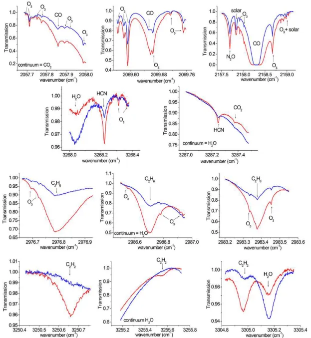
Atmospheric trace gas concentrations are retrieved using in-version procedures performed on atmospheric spectra, within suitable spectral regions, called microwindows. The choice of microwindows (MWs) is crucial because the majority of the target species have relatively weak absorptions in the in-frared region compared to the main interfering species, such as CH4, H2O and O3. All MWs have been selected in or-der to increase the information content and minimize the er-rors in the retrievals. These MWs are shown in Figs. 1 and 2, with examples of spectra recorded in clear and polluted con-ditions given in blue and red, respectively. The MWs of CO and C2H6were selected based on the recommendations of the NDACC/IRWG in their harmonization effort strategy.
The CO total columns are retrieved in three widely used MWs, including a weak line of CO at 2057.858 cm−1, an-other weak line of CO at 2069.656 cm−1 and a strong line of CO at 2158.300 cm−1(Notholt et al., 2000; Zhao et al., 2002). The use of a combination between weak and strong absorption lines increases the vertical sensitivity of the re-trievals (Barret et al., 2003). Interfering species (CO2, O3, OCS, N2O and H2O) are simultaneously scaled from their a priori profiles during the inversions. In order to obtain a good estimate of the measurement noise covariance matrix, we constructed trade-off curves of the rms residual (i.e. spec-tral fit residuals of the retrieval) versus SNR (signal-to-noise ratio) (Batchelor et al., 2009). The resulting SNR of 85 min-imized the rms residuals and maxmin-imized the DOFS (degrees of freedom for signal) of the CO retrievals.
For HCN, two MWs, around 3287.248 cm−1(Mahieu et al., 1997; Notholt et al., 2000; Zhao et al., 2002) and around 3268.200 cm−1, are preferred over the three IRWG recom-mendations (which are 3268.05–3268.40, 3287.10–3287.35
and 3299.40–3299.60 cm−1). This choice increases the in-formation content and decreases the errors in the Eureka re-trievals. The profiles of the only interfering species, H2O, are scaled from the a priori profile and an SNR of 200 is used in the retrievals.
The C2H6retrievals are performed in three MWs around 2976.800 cm−1 (Mahieu et al., 1997; Rinsland et al., 2002;
Paton-Walsh et al., 2010), 2983.300 cm−1 (Meier et al., 2004) and 2986.700 cm−1 (Notholt et al., 1997a), using an SNR of 250. Single scaling parameters are used for each of the interfering gases (H2O and O3).
For C2H2, we used three MWs, around 3250.500 cm−1 (Petersen et al., 2008), 3255.200 cm−1(Mahieu et al., 2008) and 3305.400 cm−1(Mahieu et al., 2008; Paton-Walsh et al., 2010). H2O and its main isotopologue (HDO) are scaled si-multaneously from their a priori profiles. Because the in-frared absorptions of the target gas are weak compared to the H2O lines, a reduced SNR is employed in the spectral region with no C2H2features. While an SNR of 200 is used over all the MWs, we apply an SNR of 50 between 3250.430 and 3250.550 cm−1 and between 3255.180 and 3255.455 cm−1, and an SNR of 75 from 3305.065 to 3305.350 cm−1.
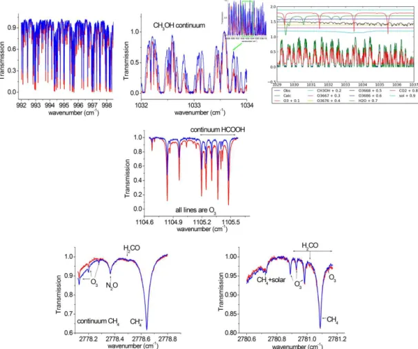
For CH3OH, we use the two MWs employed by Bader et al. (2013). In this region, the CH3OH band at 1033 cm−1 represents around 1.5 % of the absorption, whereas the O3 lines represent about 94 %. Thus, O3 and its isotopo-logues (16O18O16O labelled O686
3 ,16O16O18O labelled O6683 , 16O17O16O labelled O676
3 , and16O16O17O labelled O6673 ; Ta-ble 2) as well as the other interfering species (CO2and H2O) are retrieved simultaneously by scaling their a priori profiles. We use an SNR of 200. For more clarity in Fig. 2, we show an example of spectral fitting with the contributions of all the species in the second MW. The significant broad absorp-tion feature of CH3OH can be seen from around 1032 to 1035 cm−1(Fig. 2, right-hand panel, cyan line).
For HCOOH, we use one MW between 1104.650 and 1105.600 cm−1, which corresponds to the band used in Zander et al. (2010), Paulot et al. (2011) and Vigouroux et al. (2012). The spectroscopic parameters of this band have been updated (Perrin and Vander Auwera, 2007). Zander et al. (2010) have shown that these improvements reduce the re-trieved total columns by a factor of two. In this MW, a global SNR of 800 is used and interfering species (HDO, O3, O6683 , O676
3 , H2O, NH3, CCl2F2, CHF2Cl, CH4)are simultaneously scaled from their a priori profiles.
Figure 1.Microwindows used in the retrievals of CO, HCN, C2H6and C2H2, with examples of clear and polluted conditions in blue and red, respectively.
2.3 Retrieval methodology: optimal estimation method
In order to retrieve atmospheric concentrations from the mea-sured spectra, we use the SFIT2 algorithm (Pougatchev et al., 1995; Rinsland et al., 1998) version 3.94, which is based on a semi-empirical implementation of the optimal estimation method (OEM) of Rodgers (2000).
The inversion procedure is an ill-posed problem and re-quires the use of constraints to stabilize the solution, usually provided by the a priori information. This a priori knowl-edge is defined by the states of the atmosphere in terms of VMR vertical profiles and variabilities, for each molecule involved in the analysis (target and interfering species). The
1552 C. Viatte et al.: Five years of CO, HCN, C2H6, C2H2, CH3OH, HCOOH and H2CO total columns
Figure 2.Microwindows used in the retrievals of CH3OH, HCOOH and H2CO, with examples of clear and polluted conditions in blue and red, respectively.
The vertical information content of the retrieved profiles is quantified by the DOFS, which corresponds to the trace of the averaging kernel matrixA(Rodgers, 2000), defined as
A= ∂xˆ ∂x
=KTS−ε1K+S−a1
−1
KTS−ε1K, (1) wherexˆ andxrepresent the estimate and the true state vec-tors, respectively. Kis the weighting function matrix that
relates the measurement state to the true state of the atmo-sphere, Sε is the measurement covariance matrix and Sa is the a priori covariance matrix used in the OEM.
The spectroscopic parameters are from the HITRAN 2008 database (Rothman et al., 2009) for all the species derived in this study. As noted in Sect. 1, it contains significant im-provements concerning HCOOH and H2CO line intensities in the spectral regions of interest.
The retrieval parameters (microwindows, interfering species, a priori VMR sources, diagonal values of the a priori covariance matrix and SNRs) used for all the target species are summarized in Table 2 and discussed below.
2.4 A priori information
The location of the instrument at high latitudes offers a rel-atively dry atmosphere (total precipitable water ranges be-tween 0 and 1.8 g cm−2; Wagner et al., 2006, their Fig. 3). Compared to tropical FTIR sites, such as Reunion Island (Vigouroux et al., 2012) or Darwin in Australia (Paton-Walsh et al., 2010), our spectra are less affected by strong features due to water vapour abundance. Thus a pre-fitting of water vapour (or “two-step retrieval”) is not necessary here.
Table 2.Parameters (microwindows, interfering species, a priori VMR sources, standard deviations – SD – of the a priori covariance matrix
and signal-to-noise ratios – SNR) used in the retrievals of the seven target gases.
Target species Microwindows Interfering A priori VMR SD for SNR
species Sa(%)
Carbon CO 2057.684–2058.000, O3, CO2, WACCM v6 20 85
monoxide 2069.560–2069.760, OCS, H2O, 2157.507-2159.144 N2O
Hydrogen HCN 3268.000–3268.380, H2O WACCM v6 50 200
cyanide 3287.000–3287.480
Ethane C2H6 2976.660–2976.950, H2O, O3 WACCM v4.5 30 250
2983.200–2983.550, 2986.500–2986.950
Acetylene C2H2 3250.430–3250.770, H2O, HDO GC Toon Kiruna991203 50 200 3255.180-3255.725, Mk4-flight 6–34 km,
3304.825–3305.350 outside spitprim.set, divided by 2
Methanol CH3OH 992.000–998.700, O3, O6863 , WACCM v6 20 200
1029.000–1037.000 O6683 , O6763 , O6673 , H2O, CO2
Formic acid HCOOH 1104.650–1105.600 HDO, O3, WACCM v6 100 800
O6683 , O6763 , H2O, NH3, CCL2F2, CHF2CL, CH4
Formaldehyde H2CO 2778.120–2778.800, CH4, CO2, WACCM v6 divided by 2 100 500 2780.600–2781.170 O3, N2O
In Figs. 3 to 9 (upper panels), the a priori profiles adopted for the FTIR retrievals are shown in black, with the mean of all retrieved profiles in red. The black and red error bars correspond to the standard deviation of the a priori covari-ance matrix used in the retrievals and the standard deviations around the mean retrieved profiles, respectively, at each layer. All the a priori VMR profiles exhibit large contributions in the boundary layer and the troposphere, and decrease to al-most zero at 50 km, except for CO, for which the sources are dominated by CH4oxidation at this altitude (Clerbaux et al., 2008).
The CO a priori VMR is about 92 ppbv (1 ppbv = 10−9per unit volume) through the boundary layer, decreases to about 20 ppbv in the tropopause region and increases again with al-titude to 0.6 ppmv (1 ppmv = 10−6per unit volume) at 50 km. The HCN a priori VMR increases slightly from 25 to 32 ppbv in the troposphere and decreases in the stratosphere to reach 11 ppbv in the stratosphere. The C2H6, C2H2and CH3OH a priori VMR profiles have similar shapes as a function of al-titude. Note that the C2H6and C2H2profiles are plotted on a log scale whereas the CH3OH profile is plotted on a linear scale for clarity (Figs. 3 to 9, upper panels). Their VMRs are
almost constant in the boundary layer and the troposphere, with values of about 1 ppbv for C2H6and 0.5 ppbv for both C2H2and CH3OH. At the upper altitudes, the a priori profiles of C2H6, C2H2and CH3OH decrease until reaching∼1 pptv (1 pptv = 10−12per unit volume) at 22, 17 and 21 km, respec-tively. For HCOOH and H2CO, the a priori VMRs in the boundary layer are about 8 and 30 pptv and then decrease to 1 and 10 pptv around 30 km for HCOOH and H2CO, re-spectively. However, the sinks and sources are not as well un-derstood (Paulot et al., 2011; Jones et al., 2009), especially in the polar region, so the interpretation of the a priori profiles has to be done carefully.
1554 C. Viatte et al.: Five years of CO, HCN, C2H6, C2H2, CH3OH, HCOOH and H2CO total columns
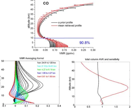
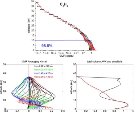
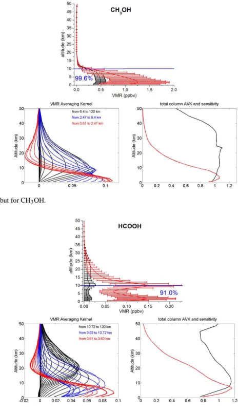
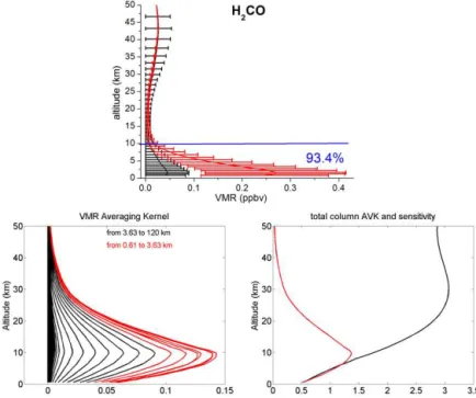
Figure 3.The CO a priori VMR profile from WACCM v6 in black (upper panel). The black error bars represent the standard deviation of
the a priori covariance matrix used in the retrievals at each layer. The mean retrieved profile is in red, with error bars corresponding to the 1σstandard deviation from the mean. The number in blue is the percentages of the tropospheric column contributions (between 0.6 and 10.7
km) relative to the total column (between 0.6 and 120 km). Typical VMR averaging kernels in VMR/VMR (lower left panel), total-column Averaging kernels (AVK) in (molecule cm−2)/(molecule cm−2) (lower right-hand panels, black line) and sensitivity profiles (right-hand panel, red line) as a function of altitude. The colours correspond to averaging kernels at altitudes lying in a partial column for which the DOFS is about 0.5.
Figure 4.Same as Fig. 3 but for HCN.
retrievals, we used a profile derived from MkIV balloon mea-surements made at the high-latitude NDACC site of Kiruna (Sweden; Toon et al., 1999), at between 6 and 34 km altitude, combined with spitprim.set (Ft. Sumner MkIV flights, 1990s,
Figure 5.Same as Fig. 3 but for C2H6. The C2H6a priori VMR profile is from WACCM v4.5.
Figure 6.Same as Fig. 3 but for C2H2. The C2H2a priori VMR profile is from MkIV balloon measurements made at the high-latitude NDACC site of Kiruna, at between 6 and 34 km altitude, combined with spitprim.set (Ft. Sumner MkIV flights, 1990s, http://mark4sun.jpl. nasa.gov/m4.html).
Instabilities in the retrieval also appear if the measured columns are substantially smaller than the a priori columns. As a result, the retrieved profile returns non-physical negative mixing ratios at the altitudes where the information content is low. This means that the most practical approach is often to use a priori profiles with a significantly lower total column
1556 C. Viatte et al.: Five years of CO, HCN, C2H6, C2H2, CH3OH, HCOOH and H2CO total columns
Figure 7.Same as Fig. 3 but for CH3OH.
Figure 8.Same as Fig. 3 but for HCOOH.
(within error bars of the measurements) when using both pro-files (that divided by two and that not divided). This confirms that the majority of the information content comes from the measurements and not from the a priori states. It is important to note that a single a priori profile for each species is used for all spectra recorded from 2007 to 2011. This ensures that our observed atmospheric variabilities mainly come from the information content of the measurements.
Figure 9.Same as Fig. 3 but for H2CO. The H2CO a priori VMR profile is from WACCM v6 and divided by 2.
The relative uncertainties of the a priori VMR profiles (or the standard deviations used in the covariance matrix) are as-sumed to be 20 % for CO and CH3OH, 50 % for HCN and C2H2, 30 % for C2H6 and 100 % for HCOOH and H2CO, at all altitude layers. These values have been scaled to ac-count for the different thicknesses of the 47 layers in our retrieval scheme. These values, summarized in Table 2, are representative of the tropospheric variabilities derived from the WACCM model, except for CH3OH and H2CO. These variabilities are, on average over the troposphere, 17 % for CO, 28 % for HCN, 30 % for C2H6and 66 % for C2H2. For CH3OH, the WACCM model suggests a high tropospheric variability of about 71 %. Since this species has broad ab-sorption features, we prefer to use a lower value of SNR in the retrievals, and then decrease the one-sigma uncertainties to 20 % in the OEM to avoid oscillations in the retrieved pro-files. In contrast, the high SNR employed in the HCOOH and H2CO retrievals, commensurate with the SNR of most analysed spectra, has been compensated for by using large values in the diagonal elements of the a priori covariance matrix. For those two species, the average tropospheric vari-abilities given by the model are 66 % for HCOOH and 39 % for H2CO. These variabilities are rather small and not con-sistent with the idea of an additional large source of HCOOH from snow photochemistry (Dibb and Arsenault, 2002) and the large H2CO variability of 30 to 700 pptv observed at the Arctic surface (De Serves, 1994).
Finally, the total columns of all the target species are rep-resentative of the tropospheric columns. The numbers in blue in Figs. 3 to 9 (upper panels) are the percentages of the tro-pospheric column contributions (between 0.6 and 10.7 km)
relative to the total column (between 0.6 and 120 km). As can be seen, the tropospheric columns make up more than 90 % of the total columns.
2.5 Averaging kernels
The rows ofA(Eq. 1) correspond to the averaging kernels
for a certain altitude layer and characterize the information content of the retrievals. An ideal observation has an averag-ing kernel of one in the region of interest and zero outside (Connor et al., 1996). Figures 3 to 9 (lower panels) present the typical VMR averaging kernels, in VMR/VMR (left pan-els), of the seven retrieved species. The different colours cor-respond to averaging kernels at altitudes lying in a partial column for which the DOFS is 0.5.
1558 C. Viatte et al.: Five years of CO, HCN, C2H6, C2H2, CH3OH, HCOOH and H2CO total columns
Table 3.Error budgets, in percentage, as a function of the different sources of random and systematic uncertainties regarding typical CO,
HCN, C2H6, C2H2, CH3OH, HCOOH and H2CO total columns retrieved at PEARL. DOFS and SZA are the acronyms of degrees of freedom for signal and solar zenith angle, respectively.
Error budget (%) CO HCN C2H6 C2H2 CH3OH HCOOH H2CO
N spectra retrieved in time series 3980 1815 1819 1269 1095 1973 1242
DOFS 2.5 1.6 2.0 1.1 1.2 1.1 0.8
Random errors
Measurement error 0.2 4.3 1.2 7 4.6 16.3 10
Uncertainty regarding temperature 0.7 0.4 0.3 2.9 4.4 2.5 5.5
Uncertainty regarding retrieval parameters 0.3 4.3 2.6 8.2 0 0 1.1
Uncertainty regarding interfering species 0 0.2 0 0.1 0 0.3 24.1
Uncertainty regarding SZA 0.3 0.3 0.3 0.7 0.2 0 0.2
Total random error 0.8 6.1 2.9 11.6 6.3 16.5 26.7
Systematic errors
Uncertainty regarding line intensity 2.9 4.9 6.4 5.7 10 3.6 2.4
Uncertainty regarding line width 0.4 3.7 2.4 7.7 1.1 0.9 2.1
Total random and systematic error 3.1 8.7 7.4 15.1 11.9 17 26.9
Smoothing error 0.2 5.9 12.2 16.7 3 1.5 5.7
Total error (random+systematic+ smoothing) 3.1 10.5 14.3 22.5 12.3 17 27.5
panels, red lines). The sensitivity at a certain altitude is the sum of the elements of the corresponding averaging kernels. It indicates the fraction of the retrievals that comes from the measurements rather than from the a priori information. A sensitivity value of one means that the information content of the retrievals is 100 % from the measurement at this altitude. All total-column averaging kernels are around one be-tween 0.6 and 10 km, which confirms the good sensitivity of our retrievals in the troposphere. Furthermore, the sensi-tivity profiles reach one in the troposphere, confirming that the majority of the information content comes from the mea-surement in this altitude region. For C2H6 and C2H2, the total-column averaging kernels and sensitivities reach zero at 36 and 22 km, respectively. As a consequence, the retrieved profiles revert to the a priori values above these altitudes (Figs. 3 to 9, upper panels).
2.6 Error budgets
Full error analyses have been performed following the for-malism of Rodgers (2000). The error budget is calculated by separating the measurement noise error, the smoothing error (expressing the limited vertical resolution of the retrieval), and the forward model parameter error (including error re-garding the temperature profiles, spectroscopic and retrieval parameters, and interfering species uncertainties, and error regarding solar zenith angles). The error analyses have been performed on a representative data set of around 10 spec-tra per species, selected with different values of solar zenith angle (SZA), SNR, hour and season of measurements. The
averages of all the calculated errors are shown for each target species in Table 3.
The measurement error covariance matrixSmis calculated as
Sm =GySεGTy, (2)
whereGyis the gain matrix representing the sensitivity of the retrieved parameter to the measurement andSε is the mea-surement covariance matrix as seen in Eq. (1). The diagonal elements ofSεare the squares of the spectral noise, which is determined by the rms residuals derived from the spectra.
The smoothing error covariance matrixSsis calculated as
Ss =(I−A)Se(I−A)T, (3)
whereIis the identity matrix,Ais the averaging kernel
ma-trix andSe is the climatology matrix representing the natu-ral variability of the target species. The lack of continuous measurements of tropospheric species in the Arctic makes it difficult to build this matrix. Thus, the values derived from WACCM have been used as diagonal elements to express the natural variabilities of each trace gas. For CO, C2H2, CH3OH, HCOOH and H2CO, the off-diagonal elements of Secorrespond to an exponential interlayer correlation with a correlation length of 4 km. For the others species, no inter-layer correlation is applied, consistent with the retrievals.
Finally the forward parameter error covariance matrixSf is calculated as
whereGy is the gain matrix andKb is the Jacobian matrix obtained by perturbation methods. Kb represents the sensi-tivity of the measurements to the model parameterb.Sb is the covariance error matrix for the parameterb. This param-eter b can have systematic (spectroscopic parameters) and random (uncertainties regarding temperature and SZA, for instance) components. To generate the Jacobians, parameters are perturbed by 0.1◦ for the error regarding SZA, by 2 K
for the temperature profiles and by a factor of 1.05 for the line intensity and air-broadened parameters (Batchelor et al., 2009).
In addition to these errors, we have examined the errors for the other retrieved parameters, called interference errors as described in Rodgers and Connor (2003) and explained in detail in Sussmann and Borsdorff (2007) and in Batchelor et al. (2009, Sect. 4). The interference errors combine the er-rors for the interfering species in the spectral region of inter-est and the uncertainty due to the retrieval parameters, such as the wavelength shift, the ILS, the background slope and curvature, the zero-level shift and the phase error.
The total random errors are calculated by adding all the un-certainties in quadrature, except the unun-certainties regarding line intensity and line width. The predominant contribution to the total random errors is the measurement error for HCN and HCOOH. For CO, the uncertainty regarding temperature is slightly higher than the uncertainty regarding the measure-ment error, but still remains small. For C2H6and C2H2, the measurement error is almost as large as the uncertainties re-garding retrieval parameters. This might be an effect of the H2O continuum, which affects the background slope and cur-vature of retrievals. For CH3OH and H2CO, the temperature uncertainty is high, which is consistent with what has been reported in Vigouroux et al. (2012) for CH3OH. Concern-ing H2CO, the largest random uncertainties come from the uncertainty regarding the interfering species. This might be explained by the fact that H2CO absorption lines are close to CH4 lines (in both MWs), which are difficult to fit be-cause of spectroscopic parameter uncertainties (Sussmann et al., 2011). This can also be an effect of the deweighting func-tion used to reduce the SNR of the interfering species in the H2CO microwindows.
The dominant contribution to the systematic error is the uncertainty regarding the line intensity for all species ex-cept C2H2, for which the line width uncertainty is larger. For H2CO, the uncertainties regarding the line width and line in-tensity are of the same order of magnitude.
As expected, the smoothing error of CO is smaller than for the other species, given the greater DOFS and the tighter averaging kernels.
Unlike the uncertainties regarding the measurement and the spectroscopic parameters, which are considered as truly random and systematic, respectively, some parameters have both components, making the division between those un-certainties difficult. Therefore, the total errors shown in
Table 3 have been determined by adding all these errors in quadrature.
Overall, the total errors of the CO, HCN, C2H2, C2H6, CH3OH, HCOOH and H2CO total columns are 3.1, 10.5, 14.3, 22.5, 12.3, 17.0 and 27.5 %, respectively.
2.7 ACE-FTS measurements
The Atmospheric Chemistry Experiment (ACE) (Bernath et al., 2005) was launched in August 2003 to investigate atmo-spheric composition mainly in the upper troposphere and the stratosphere. The ACE is equipped with a high-resolution (0.02 cm−1) Fourier transform spectrometer (FTS), operat-ing in the 750 to 4400 cm−1spectral range. It performs so-lar occultation measurements with limb geometry, with a vertical resolution of about 3–4 km (Boone et al., 2005). VMR profiles of the atmospheric species are retrieved with the version 3.0 algorithm within different altitude ranges for each molecule (http://www.ace.uwaterloo.ca/molecules. html; Boone at al., 2013). We chose ACE-FTS measurements for comparison with our new data set because the ACE has good sampling coverage at high latitudes (Bernath, 2006) and measures all seven species of interest in this study.
As shown previously, the ACE-FTS measures VMR pro-files of CO (Clerbaux et al., 2008), hydrocarbons, such as HCN, C2H6, C2H2 (Park et al., 2013) and HCOOH (González Abad et al., 2009) in the upper troposphere and lower stratosphere. In addition to these species, CH3OH and H2CO have been measured by the ACE-FTS glob-ally (Dufour et al., 2007, 2009) and in biomass burning plumes over northern high latitudes (Rinsland et al., 2007; Tereszchuk et al., 2011, 2013) and in the Southern Hemi-sphere (Coheur et al., 2007).
For comparisons with the FTIR data set, all ACE-FTS oc-cultations whose 30 km tangent altitude is within 500 km of PEARL and within 24 h of each FTIR measurement are se-lected. ACE-FTS data recorded after October 2010 are not used because of an algorithm problem in the version 3.0, which will be fixed in the future version 3.5 (Boone et al., 2013). For the calculations, each ACE-FTS profile was inter-polated to the FTIR altitude grid and the FTIR a priori pro-files were used to fill the ACE-FTS propro-files from the ground to the lowest available ACE-FTS altitudes.
The FTIR and ACE-FTS trace gas profiles are retrieved over different altitude ranges, with different vertical resolu-tions and sensitivities. To properly account for the different vertical sensitivities of the correlative observations, the ACE-FTS profiles are smoothed by convolution with the FTIR av-eraging kernel functions, following this equation (Rodgers and Connors, 2003):
1560 C. Viatte et al.: Five years of CO, HCN, C2H6, C2H2, CH3OH, HCOOH and H2CO total columns
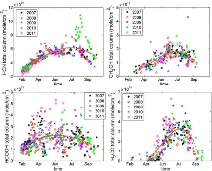
Figure 10.Daily mean total columns (in molecules cm−2) of CO, HCN and C2H6, plotted in different colours for the different years of measurements. The brown lines show the polynomial fits to the data.
Figure 11.Same as Fig. 10 but for HCN, CH3OH, HCOOH and H2CO.
Each partial column is obtained by integration of the trace gas VMR from the lowest to the highest available ACE-FTS level for both the FTIR and ACE-FTS data. Density profiles are obtained by taking the temperature and pressure profiles derived from ACE-FTS measurements.
3 Results and discussion
series of the daily mean total columns of CO, HCN, C2H6, C2H2, CH3OH, HCOOH and H2CO are plotted in Figs. 10 and 11, using different colours for the different years of mea-surements from 2007 to 2011. The brown lines represent the polynomial fits to the data. The time series are obtained dur-ing the polar-day periods since the FTIR measurements re-quire the sun as a source.
3.1 Seasonal variabilities
3.1.1 Seasonal variabilities of CO, C2H6and C2H2
The time series of the CO, C2H6 and C2H2 total columns show strong seasonal cycles with maxima in winter and min-ima in summer. These compounds are produced mainly at mid-latitudes. CO is a product of incomplete combustion and atmospheric oxidation of volatile organic compounds (VOCs) and CH4. The sources of C2H6are natural gas and fossil fuel emissions (Singh and Zimmerman, 1992). C2H2 main sources include natural gas, biofuel combustion prod-ucts and biomass burning emissions (Gupta et al., 1998; Lo-gan et al., 1981; Rudolph, 1995; Xiao et al., 2007; Zhao et al., 2002). CO, C2H6and C2H2are removed by oxidation via OH reaction (Logan et al., 1981), leading to atmospheric life-times of approximately fifty-two days (Daniel and Solomon, 1998), eighty days (Xiao et al., 2008) and two weeks in the atmosphere (Xiao et al., 2007), respectively.
The total columns of these three gases are greater in winter because their common sources, which are fossil fuel emis-sions, are usually enhanced in the dry and cold period (Zhao et al., 2002). In addition, these gases accumulate during this period because their main removal pathway is the reaction with OH, which does not take place in the dark.
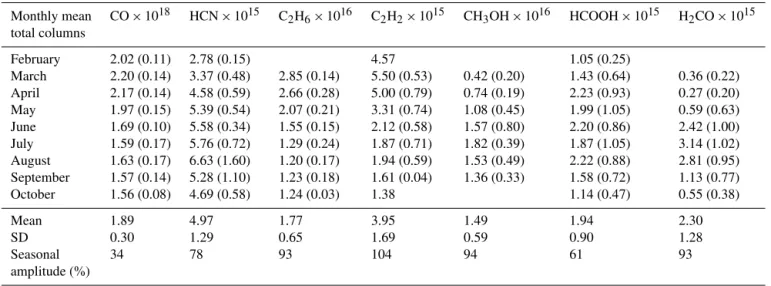
The monthly mean total columns for each species are given in Table 5. The percentages of the seasonal variability (or amplitude) are obtained by taking the difference between the maximum and minimum monthly means divided by the annual average for each gas (as described below).
The CO total columns at Eureka have a maximum in March of 2.20×10¹⁸molecules cm−2(Table 4) and a mini-mum in September of 1.56×10¹⁸molecules cm−2. The sea-sonal amplitude of CO total columns is thus estimated to be 34 %. The one-sigma standard deviation from the mean (number in parentheses in Table 4) is slightly higher for the summer months (July and August), reflecting the higher at-mospheric variability of CO due to the contribution of boreal forest fire plumes transported from lower latitudes during this period.
The C2H6 total columns have a maximum in March of 2.85×10¹⁶molecules cm−2 and a minimum in August of 1.20×10¹⁶molecules cm−2, with a seasonal amplitude of 93 %. The standard deviations around the C2H6 monthly means are larger for April and July (Table 4), certainly due to the transport of emissions from extreme fire events dur-ing these periods. This is also confirmed by the rather high
standard deviation of the well-known biomass burning tracer HCN, at this time (as described below).
For C2H2, the total columns present a maximum in March of 5.50×10¹⁵molecules cm−2 and a minimum in September-October of 1.61×10¹⁵molecules cm−2. Its sea-sonal cycle of 104 % is larger than for C2H6, in agreement with the fact C2H2 is more quickly removed by OH reac-tion (Logan et al., 1981; Singh and Zimmerman, 1992). As seen for C2H6, the standard deviations for C2H2are larger for April and July, again due to the greater transport of biomass burning plumes.
Since the lifetimes of these three molecules are rather long (from two weeks to two months, Table 1), the day-to-day variability is attributed to the long-range transport through the Arctic. For instance, the enhanced concentrations in Au-gust 2010, represented by the green dots (Fig. 10), have been attributed to an extreme fire event occurring nine days earlier in Russia and transported to Eureka (Viatte et al., 2013). To conclude, we clearly see the combined effect of the chemistry via OH reaction (seasonal variability) and transport (day-to-day variability) in the annual cycles of these three molecules in the high Arctic region.
3.1.2 Seasonal variabilities of HCN, CH3OH, HCOOH and H2CO
In contrast to CO, C2H6 and C2H2, the time series of the HCN, CH3OH, HCOOH and H2CO total columns show sea-sonal cycles with maxima in summer and minima in win-ter. HCN is a relatively inactive species and is a good tracer of biomass burning emission (Rinsland et al., 2001) with a lifetime of about five months in the troposphere (Li et al., 2003). The reaction with OH and O(1D) (Cicerone and Zell-ner, 1983) and ocean uptake (Li et al., 2003) have been shown to be the principal pathways for HCN loss, but its sinks are not well quantified yet (Zeng et al., 2012).
1562 C. Viatte et al.: Five years of CO, HCN, C2H6, C2H2, CH3OH, HCOOH and H2CO total columns
Table 4.Monthly mean total columns (in molecules cm−2) for all trace gases derived in this study from 2007 to 2011. Numbers in parentheses
correspond to the one-sigma standard deviation around the monthly mean. The three last rows show the annual means, the one-sigma standard deviation (SD) and the seasonal amplitude in percentage.
Monthly mean CO×1018 HCN×1015 C2H6×1016 C2H2×1015 CH3OH×1016 HCOOH×1015 H2CO×1015
total columns
February 2.02 (0.11) 2.78 (0.15) 4.57 1.05 (0.25)
March 2.20 (0.14) 3.37 (0.48) 2.85 (0.14) 5.50 (0.53) 0.42 (0.20) 1.43 (0.64) 0.36 (0.22) April 2.17 (0.14) 4.58 (0.59) 2.66 (0.28) 5.00 (0.79) 0.74 (0.19) 2.23 (0.93) 0.27 (0.20) May 1.97 (0.15) 5.39 (0.54) 2.07 (0.21) 3.31 (0.74) 1.08 (0.45) 1.99 (1.05) 0.59 (0.63) June 1.69 (0.10) 5.58 (0.34) 1.55 (0.15) 2.12 (0.58) 1.57 (0.80) 2.20 (0.86) 2.42 (1.00) July 1.59 (0.17) 5.76 (0.72) 1.29 (0.24) 1.87 (0.71) 1.82 (0.39) 1.87 (1.05) 3.14 (1.02) August 1.63 (0.17) 6.63 (1.60) 1.20 (0.17) 1.94 (0.59) 1.53 (0.49) 2.22 (0.88) 2.81 (0.95) September 1.57 (0.14) 5.28 (1.10) 1.23 (0.18) 1.61 (0.04) 1.36 (0.33) 1.58 (0.72) 1.13 (0.77)
October 1.56 (0.08) 4.69 (0.58) 1.24 (0.03) 1.38 1.14 (0.47) 0.55 (0.38)
Mean 1.89 4.97 1.77 3.95 1.49 1.94 2.30
SD 0.30 1.29 0.65 1.69 0.59 0.90 1.28
Seasonal 34 78 93 104 94 61 93
amplitude (%)
Table 5.Comparison of FTIR and ACE-FTS partial columns for
all trace gases derived in this study. N is the number of
coinci-dences involved in the comparison. The second column gives the mean altitude ranges used for the partial-column calculations, and the third column shows the mean distance of ACE-FTS occulta-tions to PEARL.Ris the correlation coefficient, and the fifth
col-umn gives the values of the slope of the regression plot between the FTIR partial columns and the coincident ACE-FTS measurements along with the 1σuncertainties of the slopes for each target species.
N Mean altitude Mean R Slope (FTIR range for partial distances vs. ACE-FTS)
columns (km) (km) to PEARL
CO 106 9.4–48.6 317 0.66 0.97±0.11
HCN 93 7.9–33.2 313 0.96 0.69±0.02
C2H6 17 8.0–19.3 436 0.97 0.71±0.04 C2H2 93 8.0–17.0 319 0.78 1.21±0.10 CH3OH 6 9.4–17.5 316 0.91 0.74±0.14 HCOOH 103 8.1–18.5 317 0.56 3.35±0.49 H2CO 6 9.1–38.7 317 0.75 0.50±0.22
CH3OH is the second most abundant volatile organic com-pound in the atmosphere after CH4(Jacob et al., 2005), rep-resenting 20 % of the total global VOC emissions (Guenther et al., 2006). Sources include plant growth, ocean and de-composition of plant matter as well as biomass burning emis-sion (Rinsland et al., 2009; Andreae and Merlet, 2001). The principal sink of CH3OH is chemical loss due to OH reac-tion (Heikes et al., 2002) leading to the formareac-tion of CO and H2CO (Millet et al., 2006; Rinsland et al., 2009; Stavrakou et al., 2011). The lifetime of CH3OH in the surface bound-ary layer is three to six days (Heikes et al., 2002) and be-tween five and ten days on a global scale (Jacob et al., 2005; Stavrakou et al., 2011).
Our CH3OH total columns have a seasonal amplitude of 94 % with maxima in July of 1.82×10¹⁶molecules cm−2 and minima in March of 0.42×10¹⁶molecules cm−2. This is
consistent with ACE-FTS measurements over North America and the role of vegetation growth in this region in driving its seasonal cycle (Dufour et al., 2006). However, biomass burn-ing is a significant source of CH3OH during summer and the higher standard deviations in June and August confirm the key role of enhanced plant growth and biomass burning at this time.
HCOOH is the second most abundant global organic car-boxylic acid in the atmosphere (Zander et al., 2010, and ref-erences therein). Direct sources of HCOOH include human activities, biomass burning and plant leaves, and the largest source is the photo-oxidation of NMHCs. HCOOH is re-moved through oxidation by OH as well as by dry and wet depositions (Stavrakou et al., 2012). However, a recent study suggested a missing source in the HCOOH budget of the northern latitudes and inferred its lifetime to be about three to four days (Paulot et al., 2011).
to four days; Table 1) as well as the importance of wet de-position as a sink. Indeed, the smaller standard deviations in February and March might be attributed to the lower winter atmospheric water content, decreasing the effect of wet deposition and resulting in fewer fluctuations in the HCOOH time series. During winter, total columns are affected by the short-range transport with no biogenic emission sources.
Finally, H2CO is produced by the oxidation of CH4and NMHCs, which are emitted into the atmosphere by plants, animals, industrial processes and incomplete combustion of biomass and fossil fuel. Isoprene has also been suggested as an additional significant source of H2CO (Jones et al., 2009 and references therein). In addition, secondary H2CO formation in biomass burning plumes has been proposed (Paton-Walsh et al., 2010). It is primarily removed via photo-dissociation and reaction with OH radicals with a half-life of approximately three hours in daylight (Warneck, 2000) or a lifetime of less than two days (Coheur et al., 2007).
Our H2CO total columns show a seasonal am-plitude of 93 % with summer maxima (in July of 3.14×10¹⁵molecules cm−2) and late winter minima (in April of 0.27×10¹⁵molecules cm−2). This is consistent with photochemical control by OH and its formation by CH4 oxidation in the winter seasons as well as isoprene emissions from plants and forest during the growing season. Most of the seasonal variability corresponds to the biogenic emission and biomass burning events occurring in the boreal summer months.
The seasonal cycles of CH3OH, HCOOH and H2CO in the high Arctic are driven by biogenic emissions and short-range transport from lower latitudes, whereas the biomass burning emission and long-range transport affect the seasonal variability of HCN in the Arctic.
Overall, emissions from biomass burning seem to play a significant role in the day-to-day variabilities of the seven tropospheric species observed in the high Arctic.
3.2 Comparisons with the ACE-FTS
The results of the comparisons of the FTIR measurements with those from the ACE-FTS from 2007 to 2010 are given for each molecule in Table 5.
The CO, HCN, C2H2 and HCOOH partial columns are compared with all ACE-FTS observations satisfying the co-incidence criteria defined in Sect. 2.7; this gives 106, 93, 93 and 103 pairs, respectively. The mean altitude ranges for partial-column calculations are 8.0–48.6 km for CO, 7.9– 33.2 km for HCN, 8.0–17.0 km for C2H2and 8.1–18.5 km for HCOOH. For these species, the mean distance of the ACE-FTS occultations (30 km tangent point) to PEARL is between 313 and 319 km. CO, HCN and C2H2partial columns mea-sured by the FTIR are well correlated with the ACE-FTS, with coefficients of correlation (R) of 0.66, 0.96 and 0.78. For HCOOH, the agreement is less clear since the coeffi-cient of correlation is 0.56. The FTIR C2H6partial columns,
calculated on average between 8.0 and 19.3 km, are well cor-related with the ACE-FTS data. The coefficient of correla-tion is 0.97 over 17 coincident measurements, with a mean distance to PEARL of 436 km.
The PEARL FTIR and ACE-FTS CO and C2H2 par-tial columns are in good agreement based on the slopes of the regression plots (FTIR vs. ACE-FTS). These values of 0.97±0.11 and 1.21±0.10 suggest no significant bias be-tween the two CO data sets and a positive bias in the FTIR C2H2relative to the ACE-FTS. In contrast, the FTIR HCN and C2H6 partial columns are smaller than the ones mea-sured by the ACE-FTS, given the slopes of 0.69±0.02 and 0.71±0.04, respectively. However, the FTIR HCOOH par-tial columns are significantly higher than those measured by the ACE-FTS, with a slope of 3.35±0.49.
For the CH3OH and H2CO comparisons, the small number of coincidences (N= 6) makes it difficult to draw significant conclusions. The coefficients of correlation between FTIR and ACE-FTS partial columns, calculated on average from 9.4 to 17.5 km for CH3OH and from 9.1 to 38.7 km, are 0.91 and 0.75, with slopes of 0.74±0.14 and 0.50±0.22, respec-tively. It is worth noting that 21 observations were rejected for the H2CO comparison because they were measured af-ter October 2010. The ACE-FTS algorithm version 3.5 will improve our H2CO comparisons in the future.
Given the values of the coefficients of correlation and the slopes, the Eureka FTIR measurements of CO, HCN, C2H6, C2H2and HCOOH are well correlated with ACE-FTS data, although there are biases between the two data sets, except in the case of CO. For CH3OH and H2CO, the small number of coincident profile measurements does not allow us to draw significant conclusions.
3.3 Discussion
Comparisons between our data set and previous measure-ments reported in the literature lead to a discussion of the atmospheric budget of the different target species observed in the high Arctic.
Our retrieved CO total columns (based on the five-year av-erage) are smaller by a factor of 1.3 compared to CO mea-sured at Ny Ålesund (Norway; 79◦N, 12◦E) from 1992 to
1995 (Notholt et al., 1997b). This is consistent with the de-crease of tropospheric CO of−0.61±0.16 % yr−1observed at high-latitude sites between 1996 and 2006 (Angelbratt et al., 2011). This trend has been explained by the combination of a 20 % decrease in anthropogenic CO emissions in Europe and North America and 20 % increase in CO anthropogenic emission in east Asia.
1564 C. Viatte et al.: Five years of CO, HCN, C2H6, C2H2, CH3OH, HCOOH and H2CO total columns
67◦N, 20◦E) and Harestua (Norway; 60◦N, 10◦E) from
1996 to 2006 (Angelbratt et al., 2011). Aydin et al. (2011) at-tributed this trend to the decrease of C2H6-based fossil-fuel use in the Northern Hemisphere with the possibility that an increase in chlorine atoms plays a role in the C2H6decline. Recent studies also evaluated a negative trend in the South-ern Hemisphere at Lauder (New Zealand; 45◦S, 170◦E) and
Arrival Height (Antarctica; 78◦S, 167◦E) from 1997 to 2009
as well as at Wollongong (Australia; 34◦S, 150◦E) (Zeng et
al., 2012).
For C2H2, our total-column values and seasonal variabil-ity are in agreement with values reported at Reunion Island (France; 21◦S, 55◦E) from 2004 to 2011 (Vigouroux et al.,
2012) and at Jungfraujoch station (Switzerland; 46◦N, 8◦E)
from 1995 to 2008 (Mahieu et al., 2008) as well as at Ny Ålesund from 1992 to 1999 (Albrecht et al., 2002). The sim-ilarity between high-latitude and mid-latitude C2H2 concen-trations has already been reported (Albrecht et al., 2002) and highlights the importance of transport for the C2H2 budget in the Arctic. However, the primary source of C2H2is trans-portation at mid-latitudes (Xiao et al., 2007). So the reason for the fact that our C2H2 total columns are comparable to those measured in the Arctic between 1992 and 1999 (i.e. no decrease is seen from previous years compared to the ob-served decline of CO or C2H6) is unclear. One hypothesis might be that C2H2 emissions from cars have not changed compared to the technological advances in the catalytic con-verters employed to reduce CO and C2H6emissions.
Our HCN total columns are of the same order of magni-tude, in term of absolute values and variabilities, as those reported by Notholt et al. (1997b) in the Arctic from 1992 to 1995. They also agree well with HCN columns observed at mid-latitude regions, as in northern Japan at 44◦N in 1995
(Zhao et al., 2000) as well as at Jungfraujoch from 2001 to 2009 (Li et al., 2009). In addition, our extreme values, exceeding 10×1015molecules cm−2 in summer 2010, are comparable to values found in the tropics at Reunion Is-land during the biomass burning seasons from 2004 to 2011 (Vigouroux et al., 2012). This confirms the key role of the transport from mid-latitudes in the HCN budget at high-latitudes. However, a negative trend has been highlighted in the Southern Hemisphere for the tropospheric HCN columns observed at Lauder (New Zealand; 45◦S, 170◦E) from 1997
to 2009 (Zeng et al., 2012), which is not seen in our data. This may be due to the fact that during the five years of HCN measurements at Eureka, several extreme biomass burning events were detected, especially a persistent and intense one in August 2010 (Viatte et al., 2013).
Concerning CH3OH, our total columns are of the same order of magnitude as those of Vigouroux et al. (2012) and Bader et al. (2013) obtained at Reunion Island and Jungfraujoch station, respectively. In the lat-ter study, extreme enhancements were shown to reach 2.5×10¹⁶molecules cm−2, in agreement with our high to-tal columns in the June months. Furthermore, the difference
between the largest and the smallest individual columns at Jungfraujoch station exceeds a factor of 14, which is in ex-cellent agreement with the observed variability at Eureka. Fi-nally, our monthly mean total columns show a factor of four in the seasonal amplitude, comparable to a factor three of variation found for free tropospheric CH3OH columns at Kitt Peak (United States; 32◦N, 111◦W) over 22 years of
obser-vations (Rinsland et al., 2009).
Our HCOOH retrieved columns are in agreement in terms of mean and extreme values as well as sea-sonal amplitude, compared to those measured at Jungfrau-joch (Zander et al., 2010). They reported a mean value of 1.70±0.50×10¹⁵molecules cm−2for June-July-August from 1985 to 2007, which is comparable to our average of 2.10±0.20×10¹⁵molecule cm−2 for the same summer months from 2007 to 2011. Also, our outliers are enhanced by a factor of four relative to the monthly means, which is in agreement with the large variability of HCOOH columns measured at Jungfraujoch. However, our seasonal variabil-ity is less clear than at mid-latitudes, certainly due to the contribution of the short-range transport and the importance of wet deposition as a sink of HCOOH. Finally, HCOOH total columns have been recently obtained with ground-based FTIR measurements at Thule in the Arctic (Greenland; 76◦N, 69◦W) from 2004 to 2009 (Paulot et al., 2011, their
Fig. 3). Excellent agreement, in terms of seasonal variabil-ity and extreme values, is seen with this data set, with higher values in 2008 (red circles in our Fig. 11) due to exceptional biomass burning in Asian boreal forests (Giglio et al., 2010). Finally, our H2CO total columns, which vary from 1.90×10¹³ to 6.3×10¹⁵molecules cm−2 with an annual average of 2.3×10¹⁵molecules cm−2 (between February and October), are lower than those found in the litera-ture, especially those for the spring and autumn. For in-stance, Notholt et al. (1997b) reported Arctic total columns varying from around 2 to 8×10¹⁵molecules cm−2between 1992 and 1998 at Ny Ålesund. Part of this difference might be attributed to the use of updated line strengths in HITRAN 2008. Indeed, the new spectroscopic intensities have been increased by around 30 % in the spectral region employed here (Perrin et al., 2009), leading to a signifi-cant decrease of the retrieved total columns. In addition, Jones et al. (2009) showed columns from around 2.5 to 8×10¹⁵molecules cm−2between 1992 and 2004 at Lauder (New Zealand; 45◦S, 170◦E), and Vigouroux et al. (2009)
measured columns from 1.6 to 7×10¹⁵molecules cm−2 at Reunion Island (France; 21◦S, 55◦E) between 2004 and
2011. Our low H2CO total columns measured in late winter might also reflect the large atmospheric variability of H2CO, given its small lifetime, with no local sources in winter at Eu-reka. However, our data show a strong seasonal cycle consis-tent with the FTIR measurements at Ny Ålesund (Albrecht et al., 2002) and in situ measurements at Alert (Canada; 82◦N,
4 Summary and conclusions
The ground-based FTIR technique is a powerful tool for deriving long-term measurements of various atmospheric species having both natural and anthropogenic sources. Mon-itoring tropospheric molecules with different atmospheric lifetimes and origins provides useful information about chemical and physical processes in the Arctic, such as trans-port (Shindell et al., 2008) and the degradation mechanisms of non-methane hydrocarbons (Stavrakou et al., 2009), which need to be better understood in model simulations (Millet et al., 2008; Parker et al., 2011; Paulot et al., 2011). Our ground-based FTIR measurements at PEARL constitute a new Arctic data set of seven tropospheric species, CO, HCN, C2H6, C2H2, CH3OH, HCOOH and H2CO, observed from 2007 to 2011. The total columns of CH3OH are the first to be reported from ground-based FTIR measurements in the high Arctic.
The different lifetimes of these tropospheric molecules, from less than two days to six months, play a role in their observed seasonal variabilities at PEARL. The seasonal vari-ability provides additional evidence of the interplay between chemistry and transport, which will help to constrain global atmospheric chemical transport models. The time series of the CO, C2H6and C2H2total columns show strong seasonal amplitudes of 34, 93 and 104 %, respectively, with maxima in winter and minima in summer. These seasonal cycles high-light the combined effect of the chemistry via OH reaction (seasonal variability) and long-range transport (day-to-day variability) in the Arctic budget of CO, C2H6 and C2H2. In contrast to these molecules, the time series of the HCN, CH3OH, HCOOH and H2CO total columns show seasonal amplitudes of 78, 94, 61 and 93 %, respectively, with max-ima in summer and minmax-ima in winter. These seasonal cycles are driven by biogenic emissions and short-range transport for CH3OH, HCOOH and H2CO, and biomass burning emis-sions and long-range transport for HCN. Overall, emisemis-sions from biomass burning seem to play a significant role in the day-to-day variability of the seven tropospheric species ob-served in the high Arctic. This data set highlights the impor-tance of the transport of pollutants from lower latitudes and can be used to assess the influx of pollution into the sensitive area of the Arctic.
In order to assess our new data set, the ACE-FTS satel-lite instrument was selected since it has good sampling in the Arctic and measures all seven species studied here. Given the values of the coefficients of correlation and the slopes, rang-ing from 0.56 to 0.97 and from 0.71 to 3.35, respectively, the FTIR measurements at Eureka of CO, HCN, C2H6, C2H2 and HCOOH are generally well correlated with the ACE-FTS data, although there are biases between the two data sets. For CH3OH and H2CO, the small number of coincidences (six pairs) does not allow us to draw meaningful conclusions.
Finally, our new data set has been compared to previous published measurements. Our measurements are consistent with the negative trends of CO and C2H6observed over the Northern Hemisphere, which have been attributed to decreas-ing fossil fuel emissions. The similarity of the HCN and C2H2concentrations between mid- and high latitudes high-lights the importance of transport for the atmospheric bud-get of these molecules in the Arctic. Concentrations and sea-sonal cycles of CH3OH and HCOOH at PEARL are com-parable with previous measurements performed at remote sites. Excellent agreement is found between our HCOOH total columns and measurements from Thule (Paulot et al., 2011). However, the atmospheric concentrations of H2CO at PEARL in the early spring are smaller than those reported in the literature. This might reflect the large atmospheric vari-ability of H2CO, given its short lifetime with no local sources in winter at Eureka, and/or the effect of the updated spectro-scopic parameters used in our retrievals.
To conclude, our measurements of tropospheric species at Eureka constitute a new data set which can be used as a constraint to improve the model simulations of chemical and dynamical processes in the high Arctic. Comparisons of the FTIR measurements with two chemical-transport mod-els are in progress. In addition, since all seven molecules are biomass burning products, they can be used to identify fire events in order to study the chemical composition of the plumes above PEARL and to derive emission ratios, which are key parameters needed to simulate fire emissions in at-mospheric models.
Acknowledgements. The PEARL Bruker 125HR measurements at
Eureka were carried out by the Canadian Network for the Detection of Atmospheric Change (CANDAC), which was supported by the Atlantic Innovation Fund/Nova Scotia Research and Innovation Trust, the Canada Foundation for Innovation, the Canadian Foun-dation for Climate and Atmospheric Sciences, the Canadian Space Agency (CSA), Environment Canada, Government of Canada Inter-national Polar Year funding, the Natural Sciences and Engineering Research Council of Canada, the Ontario Innovation Trust, the Ontario Research Fund, and the Polar Continental Shelf Program. The authors wish to thank the staff at Environment Canada’s Eureka Weather Station and CANDAC for logistical and on-site support. Thanks to Rodica Lindenmaier, Rebecca Batchelor and PEARL Site Manager Pierre Fogal as well as CANDAC/PEARL operators Ashley Harrett, Alexei Khmel, Paul Loewen, Keith MacQuarrie, Oleg Mikhailov and Matt Okraszewski for their invaluable as-sistance in maintaining and operating the Bruker 125HR. The Atmospheric Chemistry Experiment is a Canadian-led mission mainly supported by the CSA.