www.j-sens-sens-syst.net/4/217/2015/ doi:10.5194/jsss-4-217-2015
© Author(s) 2015. CC Attribution 3.0 License.
Increasing the sensitivity of electrical impedance to
piezoelectric material parameters with non-uniform
electrical excitation
K. Kulshreshtha1, B. Jurgelucks1, F. Bause2, J. Rautenberg2, and C. Unverzagt2 1Institut für Mathematik, Universität Paderborn, Warburger Str. 100, 33098 Paderborn, Germany 2Elektrische Messtechnik, Universität Paderborn, Warburger Str. 100, 33098 Paderborn, Germany
Correspondence to:K. Kulshreshtha ([email protected])
Received: 18 February 2015 – Revised: 16 April 2015 – Accepted: 6 May 2015 – Published: 12 June 2015
Abstract. To increase the robustness and functionality of piezoceramic ultrasonic sensors, e.g. for flow, ma-terial concentration or non-destructive testing, their development is often supported by computer simulations. The results of such finite-element-based simulations are dependent on correct simulation parameters, especially the material data set of the modelled piezoceramic. In recent years several well-known methods for estimation of such parameters have been developed that require knowledge of the sensitivity of a measured behaviour of the material with respect to the parameter set. One such measurable quantity is the electrical impedance of the ceramic. Previous studies for radially symmetric sensors with holohedral electrode setups have shown that the impedance shows little or no sensitivity to certain parameters and simulations reflect this behaviour making pa-rameter estimation difficult. In this paper we have used simulations with special ring-shaped electrode geometry and non-uniform electrical excitation in order to find electrode geometries, with which the computed impedance displays a higher sensitivity to the changes in the parameter set. We find that many such electrode geometries exist in simulations and formulate an optimisation problem to find the local maxima of the sensitivities. Such configurations can be used to conduct experiments and solve the parameter estimation problem more efficiently.
1 Motivation
Piezoelectric effect is the physical phenomenon discovered by Pierre and Jacques Curie in 1880 that is exhibited by sev-eral crystalline and synthetic ceramic materials. When volt-age is applied across certain surfaces of the solid, it exhibits mechanical strain; conversely, when mechanical stresses are applied, voltage is produced between its surfaces.
Acoustic transducers are required to construct an ultra-sonic measurement device of any kind. Transducers based on circular piezoelectric ceramic disks have been manufactured and used in a wide variety of applications.
Ceramics are composed of a large number of randomly oriented crystals. The cumulative properties of each of these crystals together determine the properties of the whole solid. This means that each batch of the ceramic produced will have somewhat different material properties. Additionally, the
ma-terial coefficients are dependent on geometry. If a such a ce-ramic disk with a specific thickness and diameter is sintered and polarised, the resulting material coefficients are differ-ent than a disk of the same material and of differdiffer-ent thick-ness and diameter. Hence, post processing and treatment of the material also influences the material coefficients. Pérez et al. (2010) found the elastic coefficients to vary up to 5 % and the piezoelectric and dielectric coefficients to vary up to 20 %. These variations include measurement uncertainties concerning the determination of the coefficients and also the batch-to-batch and geometry dependencies.
Depending on the application at hand, the full knowledge of the material data set can be crucial to the whole process: for a circular disk with full width electrodes on the top and bottom (see Fig. 1) there is no shear movement; hence,e15is
~
V
L
Figure 1.Two-electrode configuration on a circular disk (Lahmer, 2008).
Analytical and numerical modelling of piezoelectricity and the resulting computer simulations (Kocbach, 2000; Un-verzagt et al., 2013) have enabled more efficient design and construction of transducers in recent years.
Such numerical modelling requires the precise knowledge of the parameters of the material under analysis. To this end, new methods that utilise the mathematical concept of inverse problems to estimate the material parameters have been de-signed (Kaltenbacher et al., 2006, 2008).
Previous studies (Rautenberg et al., 2011) have shown that configurations inducing resonance in radial or thickness di-rections (Lahmer, 2008) are insufficient for parameter es-timation, when only the electrical impedance is measured, because the impedance characteristic in the frequency space shows little or no sensitivity to certain material parameters. Especially critical are c44,ε11 ande15 since in the
experi-ments of Rautenberg et al. (2011) they show no sensitivity to material parameters at all. Low or no sensitivity means that these parameters cannot be estimated using inverse problems from the measurement of impedance characteristics only. Other, more involved measurements have been proposed in Rupitsch et al. (2009); however, they are also much more cost-intensive.
In order to improve the sensitivity of the measured impedance characteristic to the material parameters, we de-signed a three-electrode configuration with electrodes of var-ious radii as shown in Fig. 2a and b and use simulations in which a non-uniform electrical excitation is applied to the ce-ramic in order to compute the impedance characteristic and its sensitivity to the material parameters.
Possible applications with non-uniform electrical excita-tion in piezoelectric ceramics are interdigital transducers (Kirschner, 2010) and annular arrays (Ketterling et al., 2005; Ramli and Nordin, 2011).
In the following sections we first give a short overview of the equations governing our simulation and the excitation of the ceramic. We then define and analyse the sensitivity of the computed impedance to parameters. Finally, we formulate an optimisation problem to find a locally optimal electrode ge-ometry that maximises the sensitivity and show that many such local optima occur.
V1
V2
(a)
V1
V2
(b)
C
R Z
Z Z
V 1
2
V 2
0 a
b c R2
(c)
Figure 2.(a)Arrangement of electrodes in thin rings;(b) arrange-ment of electrodes in wide rings;(c)schematic diagram of the whole circuit with the piezoceramic shown as a T-Network.
2 Modelling piezoelectricity
In this paper we restrict ourselves to linear piezoelectric ef-fect IEEE Std 176-1987. The equations of linear piezoelec-tricity in tensor form are given below and form the basis for a finite-element formulation.
σ =cS−e⊤E, (1)
D=eS+εE, (2)
where
– Dis the electrical flux density vector
– Eis the electrical field vector – σis the mechanical stress tensor
– Sis the mechanical strain tensor
– cis elastic modulus tensor
– eis the piezoelectric coupling tensor
– εis the electrical permittivity tensor.
and Lahmer (2008) (Voigt notation) in the rotationally sym-metric case we can rewrite the tensor notation into matrix formulation: c=
c11 c13 0 c12
c13 c33 0 c13
0 0 c44 0
c12 c13 0 c11 , e=
0 0 e15 0
e13 e33 0 e13
,
ε=
ε11 0
0 ε33
.
This results in the following system of material equations from Eqs. (1) and (2):
σrr σzz σrz
σθ θ
Dr Dz =
c11 c13 0 c12 0 −e13
c13 c33 0 c13 0 −e33
0 0 c44 0 −e15 0
c12 c13 0 c11 0 −e13
0 0 e15 0 ε11 0
e13 e33 0 e13 0 ε33
Srr Szz Srz Sθ θ Er Ez . (3)
The above material equation can be extended to a full set of partial differential equations in time and space using New-ton’s, Gauss’ and Faraday’s Laws (Meschede and Gerthsen, 2010, Chap. 4 and Chap. 7).
Newton’s law of motion (Slaughter, 2002, Cauchy-Navier equation) for the mechanical behaviour is
B⊤σ =̺∂
2u
∂t2, (4)
whereBis the differential operator relating mechanical strain
to mechanical displacement.
B=
∂r 0 0 ∂z ∂z ∂r
1 r 0
As ceramic materials are insulators, there is no free charge and Gauss’ (flux) law states
∇ ·D=0. (5)
Neglecting the insignificant changes in magnetic field in this case, Faraday’s law states that the electric field is the negative gradient of the electric potential.
E= −∇φ (6)
Additionally, we consider a Rayleigh damping model with positive constantαandβ for the energy dissipation and ar-rive at a system of four partial differential equations in time
and space from Eqs. (3), (4), (5) and (6): ̺u¨+α̺u˙−B⊤(cBu+βcu˙+e⊤∇φ)
=0 in , t∈ [0, T], (7)
∇ ·(eBu−ε∇φ)=0 in. (8) These equations are sufficient for transient analysis. The electrodes and their excitation occur as boundary conditions, in terms of free charge
qL= Z
ŴL ˆ
n·(eBu−ε∇φ)dŴ (9)
at the part of the boundary containing the electrodeŴLwith ˆ
nbeing the normal vectornˆ=(nr, nz)⊤at the boundary, or the applied potentialφL(t) at the electrodeL. We call the remaining boundaryŴr=ŴrŴL.
The above equations may also be transformed for har-monic analysis into the frequency domain. Application of a Fourier transform changes the unknownsuandφin Eqs. (7) and (8) to time harmonic complex variablesuˆ andφˆ, and the Rayleigh coefficients are scaled according to frequency.
α(ω)=α0ω, β(ω)=
β0
ω
The resulting time harmonic partial differential equations are given as follows:
−̺ω2uˆ− 1 1−ıα0
B⊤(1+ıβ0)cBuˆ+e⊤∇ ˆφ
=0 in, (10)
∇ ·eBuˆ−ε∇ ˆφ=0 in, (11)
withıbeing the imaginary unit.
This transformation however contains a systematic error asα0andβ0are not constants in practice but change with the
central frequency of the Fourier transform.
Weak formulations and finite-element methods for the so-lution of the above system have been studied in Kocbach (2000) and Lahmer (2008).
3 Electrical excitation
In order to simulate the behaviour of a piezoelectric trans-ducer with finite elements, it is excited by a delta function of the charge or a pulse of potential. This gives the boundary conditions to solve Eqs. (7) and (8).
Electrical current flow at the electrode is the time deriva-tive of the free charge and the impedance between any two electrodes is then defined as the quotient of the potential dif-ference and the current. In the simple case of two electrodes, with a delta function pulse of charge into one electrode with amplitudeq0L,
(see Fig. 1), this leads to the straightforward calculation
ZL(ωk)= ˆ
φL(ωk) q0L ,
whereωk is some frequency of interest,qˆ0Ldenotes the fre-quency domain charge peak andφˆL(ωk) is the calculated re-sponse of the potential difference using Eqs. (7) and (8).
In our setup two different electric potentials are applied on two electrodes and the third is grounded. An external circuit (Fig. 2c) is required to achieve this potential differ-ence at the electrodes. The values of the resistorsR0andR2
and capacitorC2 are chosen to maintainV1≥2V2. This is
done by solving the equations of Kirchhoff’s laws for the circuit (Meschede and Gerthsen, 2010, Chap. 7). As the cir-cuit representation of the ceramic includes three unknown impedances, the solution of the Kirchhoff laws equations re-quires three finite-element solutions for Eqs. (7) and (8) using an initial guess for the material parameters and a given elec-trode geometry (Unverzagt et al., 2015). The chosen values for the external circuit are then kept constant for that partic-ular electrode geometry, while we compute the sensitivity of the total impedance to material parameters and optimise it as discussed in Sect. 5.
4 Sensitivity
For each frequency of interest in the domain, the solution of Eqs. (7) and (8) along with the external circuit results in a total impedance, which can be measured in experiments and compared with the numerical computations in order to es-timate the material parameters (Rupitsch and Lerch, 2009; Kaltenbacher et al., 2008). The first step to solve this inverse problem requires the determination of a sensitivity of the nu-merical solution to variations in the material parameters. This is in fact the derivative of the impedance with respect to the material parameters.
For the numerical solution we use the commercial soft-ware package CAPA, which computes the impedance for a given configuration. CAPA is a simulation tool for the nu-merical solution of electromechanical, coupled field prob-lems and is therefore suitable for the analysis of most mecha-tronic sensors and actuators such as electromagnetic loud-speakers or piezoelectric transducers.
Besides transient analysis, which is used in this contribu-tion, the harmonic behaviour of the piezoceramic disc can also be calculated. One disadvantage of the transient simula-tion method is the sole use of the Rayleigh damping model for the energy dissipation processes as mentioned in Sect. 2. This is a rather simple approximation of the damping be-haviour in practice. Another disadvantage of precompiled solver packages in general is inflexibility; it is impossible to modify the computation in any way in order to be able to compute more information, like sensitivities.
In contrast to previous studies we look at the real and imaginary parts of the complex impedance separately in-stead of looking at the magnitude. The formulation in terms of magnitude and phase, although computationally efficient, hides some geometrical structure, which is apparent when looking at the real and imaginary components separately. This is analogous to a polar coordinate system versus a cartesian coordinate system. Figure 3a shows the complex impedance as a function of the frequency in the com-plex plane, whereas Fig. 3b shows the magnitude of the impedance. The 3-D plot shows more structure and we use the same representation for the sensitivities.
We used finite-difference approximations for the config-uration in Fig. 8 for the sensitivity of the impedance w.r.t. the material parameters. Figure 4 shows the sensitivity of the impedance in the frequency domain w.r.t.c44,e15 andε11
(occurring in Eq. 3) that are known to show low sensitivity in simpler configurations (Rautenberg et al., 2011).
Using a slightly different geometry (see resulting geom-etry in Table 1) for the electrodes but the same excitation, the sensitivity curves change both qualitatively and quanti-tatively (see Fig. 6 and compare with Fig. 4). However, the change is not uniform across the parameters. Hence, there is a need to find the optimal electrode configuration to ensure maximal sensitivity of the impedance to the material param-eters.
5 Optimisation
We start by formulating a constrained minimisation problem with the electrode radii as the variables which will then be solved.
The electrode configuration is parametrised using four ring radiir=(r1, . . ., rNr =r4) and considering the outer radius as constant (see Fig. 5). Letx=(x1, . . ., xN
x) denote the var-ious material parameters occurring in Eq. (3) and letF⊆R
denote the frequency domain. The impedanceZ(f;x,r) can
be considered as a functionZ:F×RNx×RNr →C. For
fixed radii parametrisationr and material parametersx the
impedance is a functionZ(f;x,r):F→Cwhich maps the
argument f 7−→Z(f;x,r). This complex-valued function
Z is then transformed into a two-dimensional real function z(·;x,r):F→R2via the usual Euclidean mapping. We
ap-proximate the partial derivative ofztowards a change of ma-terial parameterxi using a finite-differences scheme
∇xiz(·;x,r)≈
z(·;xi+h,r)−z(·;x,r)
h ∈ {F→R
2 }
with xi+h:=(x1, . . ., xi−1, xi+h, xi+1, . . ., xNx) and for smallh >0. Hence, the sensitivity ofztowards one specific parameterxiwhile remaining in a constant electrode config-urationrcan be considered as∇xiz(·;x,r)
L2(F). We
con-sider the norm of the corresponding function spaceL2(F) to
0 1
2
x 106
100 150 200 250 −100 −50 0
ℑ
(
Z
)
/
Ω
ℜ(
Z)/
Ω f/Hz
(a)
0 0.5 1 1.5 2 2.5
x 106
160 180 200 220 240
|
Z
|
/
Ω
N
/
C
f /Hz
(b)
Figure 3.(a)Complex impedance vs. frequency;(b)magnitude of impedance vs. frequency.
0 1
2
x 106 −2000
0 2000 −1000 0 1000 2000
ℑ
(
∂
Z
∂
c44
)
/
Ω
m
2/
N
ℜ( ∂ Z ∂c
44)/Ω
m2
/N f/Hz
(a)
0 1
2
x 106 −100
0 100 200 −100 0 100
ℑ
(
∂
Z
∂
e15
)
/
Ω
N
/
C
ℜ( ∂ Z ∂e
15)/
Ω
N/C f/Hz
(b)
0 1
2
x 106 −10
0 10 20 30 −10 0 10
ℑ
(
∂
Z
∂
ǫ11
)
/
m
Ω
2/
s
ℜ( ∂ Z
∂ǫ 11)/
mΩ2
/s f/Hz
(c)
Figure 4. Sensitivity of the impedance for the geometry of the ring electrodes shown in Fig. 8 to various material parameters against frequency w.r.t.(a)c44,(b)e15, and(c)ε11.
r
2r
1R
=
const
.
r
3r
4Figure 5.Parametrisation of the ring radii compared with Fig. 4. However, the change is not uniform across the parameters. Hence there is a need to find the optimal electrode configuration to ensure maximal sensitivity of the impedance to the material parameters.
∇xiz(·;x,r) L2(F)=
Z
F
k∇xiz(f;x,r)k 2 2df
1 2
.
Discretising the frequency domainFequidistantly into
0 1
2
x 106
−1000 0 1000 −1000
0 1000
ℑ
(
∂
Z
∂
c44
)
/
Ω
m
2/
N
ℜ( ∂ Z ∂c
44)/Ω
m2
/N f/Hz
(a)
0 1
2
x 106
−100 0 100 200 −100 0 100
ℑ
(
∂
Z
∂
e15
)
/
Ω
N
/
C
ℜ( ∂ Z ∂e
15)/Ω
N/
C f/
Hz
(b)
0 1
2
x 106
−20 0 20 −10 0 10 20
ℑ
(
∂
Z
∂
ǫ11
)
/
m
Ω
2/
s
ℜ( ∂ Z
∂ǫ 11)/
mΩ2
/s f /Hz
(c)
Figure 6.Sensitivity of the impedance for the resulting geometry of the ring electrodes shown in Table 1 to various material parameters against frequency w.r.t.(a)c44,(b)e15, and(c)ε11.
∇xiz(·;x,r) L2(F)
≈
ˆ
h 2
X
1≤i≤Nf−1
|∇xiz(fi+1)| 2
+ |∇xiz(fi)| 2
1 2
.
Now, we wish to maximise the sensitivities
∇z(r)=h∇xjz(·;x,r)
L2(F) i
j=1,...,Nx
with respect to all material parametersxi.
We have noticed that some parameters are very reactive towards change in geometry and others are not. Due to un-evenly distributed sensitivity of the material parametersx
to-wards optimisation, their different orders of magnitudes and the circumstance that the optimisation method used may only minimise an objective function, we introduce a weight ma-trixW:=diag(w1, . . ., wNx)∈R
Nx×Nx
+ and a scaling matrix
S:=diag(s1, . . ., sNx)∈R
Nx×Nx depending on the orders of magnitude of the initial sensitivity evaluation and reformu-late the sensitivity approximation as the minimisation prob-lem:
minrJ(r)=minr
1 kW S∇z(r)k2 =minr=(r1,...,rNr)
1
W Sh∇xjz(·;x,r)
L2(F) i
j=1,...,Nx 2
2
.
The scaling is only used inside the optimiser so that all components of the gradient have a similar scale and has no meaning outside the optimisation routine. For comparison of the results one needs to compare the unscaled objective func-tion withS=I, the identity matrix.
5.1 Constraints
Table 1. Uniform weights: improvement of sensitivity of impedance w.r.t material parameters usingW=diag(1, . . .,1). The sensitivity has increased for all the parameters with exception of
e15. These are the best component-wise results we have computed so far. Objective function values are shown unscaled. Figure shows resulting geometry utilising uniform weight matrix in millimetres;
r1=4.01;r2=4.33;r3=2.20;r4=3.82.
Param. W Start Optimal Gain ratio
c11 1 2.0770×10³ 6.3875×10³ 3.0753
c33 1 803.3076 2.0959×10³ 2.6091
c44 1 1.9901×10⁴ 2.0009×10⁴ 1.0054
c12 1 0.6624 0.8330 1.2575
c13 1 4.4700×10³ 1.2292×10⁴ 2.7500
ǫ33 1 1.4591 2.1917 1.5021
e31 1 83.2714 254.6764 3.0584
e33 1 62.9616 149.2692 2.3708
ǫ11 1 3.6831 4.6061 1.2506
e15 1 262.1774 246.1737 0.9390
Obj. 2.3748×10⁻⁹ 1.6756×10⁻⁹ 0.7056
k∇Zk2 4.2109×10⁸ 5.9681×10⁸ 1.4173
−5
0
5
−2
0
2
mm
mm
r
1r
2r
3r
4weights: Improvement of sensitivity of impedance w.r.t material parameters
A:=
1 0 0 0
0 1 0 0
0 0 1 0
0 0 0 1
−1 0 0 0
0 −1 0 0
0 0 −1 0
0 0 0 −1
1 −1 0 0
0 0 1 −1
, b:=
4.985 4.685 4.985 4.985 −0.15
0 −0.15
0 −0.3 −0.3
.
Table 2.Binary weights: improvement of sensitivity of impedance w.r.t. material parameters usingW=diag(0,0,0,0,0,0,0,0,0,1). The sensitivity w.r.te15has increased. However, the sensitivity to-ward other parameters has mainly decreased. Objective function values are shown unscaled. Figure shows resulting geometry util-ising binary weight matrix in millimetres;r1=3.4;r2=3.7;r3=
1.23;r4=3.54.
Param. W Start Optimal Gain ratio
c11 0 2.0770×10³ 1.7465×10³ 0.8409
c33 0 803.3076 670.3565 0.8345
c44 0 1.9901×10⁴ 1.9167×10⁴ 0.9631
c12 0 0.6624 0.6789 1.0248
c13 0 4.4700×10³ 3.8569×10³ 0.8628
ǫ33 0 1.4591 1.2413 0.8507
e31 0 83.2714 67.8750 0.8151
e33 0 62.9616 47.5998 0.7560
ǫ11 0 3.6831 4.3195 1.1728
e15 1 262.1774 344.2983 1.3132
Obj. 1.4548×10⁻⁵ 8.4359×10⁻⁶ 0.5799
kW∇Zk2 6.8737×10⁴ 1.1854×10⁵ 1.7246
−5
0
5
−2
0
2
mm
mm
r
1r
2r
3r
4weights: Improvement of sensitivity of impedance w.r.t. material parameters
Hence, the resulting minimisation problem is stated as
min
r
1
kW S∇z(r)k2w.r.t.A r≤b.
5.2 Optimisation method
Since the sensitivity itself is a finite-difference approxima-tion, it makes little sense to use an optimisation method that requires further derivatives. For the optimisation we used Powell’s latest derivative-free trust region optimiser LIN-COA (LINearly Constrained Optimization Algorithm) (Pow-ell, 2014a, b) for linearly constrained problems.
The LINCOA method is a derivative-free optimisation al-gorithm for linearly constrained problems written in Fortran by M.J.D. Powell. It is based on Powell‘s other derivative-free optimisation algorithms with the distinction of incorpo-rating general linear constraints. However, a detailed descrip-tion of the LINCOA software has not been published yet.
According to Powell (2014a), the LINCOA method uses a quadratic model
Q(x)=c+gTx+1 2x
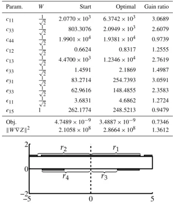
Table 3.Mixed weights: improvement of sensitivity of impedance w.r.t. material parameters usingW=√1
2·diag(1, . . .,1,
√
2). With exception ofc44ande15all partial sensitivities are increased. Ob-jective function values are shown unscaled. Figure shows result-ing geometry utilisresult-ing mixed weight matrix in millimetres; r1= 4.01;r2=4.34;r3=2.17;r4=3.93.
Param. W Start Optimal Gain ratio
c11 √12 2.0770×10³ 6.3742×10³ 3.0689
c33 √12 803.3076 2.0949×10³ 2.6079
c44 √12 1.9901×10⁴ 1.9381×10⁴ 0.9739
c12 √12 0.6624 0.8317 1.2555
c13 √12 4.4700×10³ 1.2346×10⁴ 2.7619
ǫ33 √12 1.4591 2.1869 1.4987
e31 √12 83.2714 254.7393 3.0591
e33 √12 62.9616 148.4855 2.3583
ǫ11 √12 3.6831 4.6862 1.2724
e15 1 262.1774 248.5213 0.9479
Obj. 4.7489×10⁻⁹ 3.4887×10⁻⁹ 0.7346
kW∇Zk2 2.1058×10⁸ 2.8664×10⁸ 1.3612
−5 0 5
−2 0 2
r
1r
2r
3r
4as an approximation to the objective function J(x)∈Rn. However, as no derivatives are available, the quadratic model Qhas to be iteratively constructed from function evaluations ofJ. At the beginning of the optimisation, the user chooses the amount of pointsmwhich are further used to interpolate the modelQwithm∈ {n+2, . . .,21(n+1)(n+2)}, a typical choice formbeing 2n+1. This leaves 12(n+1)(n+2)−m degrees of freedom for the choice ofQwhich are fixed by ap-plying a symmetric Broyden updating method to the model Q. A trust region and an active-set approach incorporating the linear constraints then determine the new points for up-dating the model functionQ, which is iteratively minimised by the process. The trust region size in the process is de-creased when certain conditions are fulfilled until ultimately the algorithm halts as the trust region size has reached a user-prescribed lower boundary.
5.3 Results
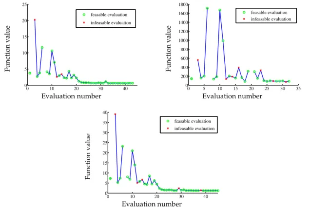
In the following section we will present results of the sen-sitivity optimisation. The section is divided into two parts. In the first part we will concentrate on the influence of the weight matrixW on the optimisation. We have tested differ-ent weight assignmdiffer-ents (uniform, binary and mixed) forW
Table 4. Different starting configurations with uniform weight
W=diag(1, . . .,1). Initial electrode configurations for case in (a):
r= [0.30.64.44.7]; for case in (b):r= [2.02.30.34.7]; for case in (c):r= [0.34.682.052.35]. Successful optimisation of overall and partial sensitivities, however, sensitivity ratio to optimised reference (∗SROR) initial point shows that the results are not that good. Ob-jective function values are shown unscaled.
Param. Gain ratio SROR∗
(a) Obj. func. : 4.0978×10⁻⁷.
k∇Zk2= 2.4403×10⁶
c11 1.2434 0.0849
c33 1.4205 0.1292
c44 5.3202 0.3028
c12 1.0125 0.2835
c13 1.0978 0.0855
ǫ33 1.3629 0.3185
e31 1.1556 0.0947
e33 1.8522 0.1520
ǫ11 2.8385 0.2002
e15 3.2481 0.3084
(b) Obj. func. : 1.5881×10⁻⁹.
k∇Zk2= 6.2967×10⁸
c11 0.9293 0.2234
c33 0.8531 0.3203
c44 1.1749 1.2426
c12 0.5684 1.1232
c13 0.8933 0.2433
ǫ33 0.6659 0.7925
e31 1.0677 0.1759
e33 0.9212 0.2585
ǫ11 1.2864 0.5104
e15 1.4586 0.9625
(c) Obj. func. : 5.7492×10⁻⁸.
k∇Zk2= 1.7394×10⁷
c11 1.1830 0.0068
c33 2.3508 0.0271
c44 4.3539 0.2084
c12 2.6384 0.0748
c13 1.3414 0.0073
ǫ33 2.5290 0.0877
e31 1.2714 0.0109
e33 2.4383 0.0705
ǫ11 2.0128 0.1069
e15 1.8070 0.0977
0 10 20 30 40 0
5 10 15 20 25
feasable evaluation infeasable evaluation
Function
value
Evaluation number
0 5 10 15 20 25 30 35 0
200 400 600 800 1000 1200 1400 1600 1800
feasable evaluation infeasable evaluation
Function
value
Evaluation number
0 10 20 30 40
0 5 10 15 20 25 30 35 40
feasable evaluation infeasable evaluation
Function
value
Evaluation number
Figure 7.Evaluation history for uniform weights, binary weights, and mixed weights. Initial values are 3.7283, 145.45821 and 7.2703; optimised values are 0.6219, 84.3588 and 1.2397, respectively.
−5
0
5
−2
0
2
r
1r
2r
3r
4Figure 8.Reference initial geometry in millimetres;r1=3.5;r2= 3.8;r3=2.05;r4=3.55.
Influence of the weighting matrix
As an initial point for a first optimisation we used the elec-trode configuration of a piezoceramic (see Fig. 8) we phys-ically possess for measurement purposes. This ceramic con-figuration has been developed in Unverzagt et al. (2015) us-ing statistical methods. We have made the experience that this configuration has exceptionally good properties with re-gard to optimisation as opposed to other geometries tested. We shall call this configuration the reference initial point. For the optimisation process we used the uniform weights W =diag(1, . . .,1). A summary of the results can be found in Table 1 along with the final geometry. This shows an overall increase in sensitivityk∇Zk2by more than 41 % and some partial sensitivities were increased by up to 307 %. However,
not all partial sensitivities are very reactive towards changes in the electrode configuration, i.e. the sensitivity gain regard-inge15is−6.1 %.
As a reaction to this slight partial decrease in sensitivity regardinge15we chose to neglect the partial sensitivities of
those parameters which have a positive gain and focus on e15 by setting the corresponding weights to 0 and 1,
respec-tively. Through this binary weight-matrix setting, the sensi-tivity with regard toe15was increased by 31 %. (see Table 2)
However, following our expectations, the sensitivities regard-ing the other parameters have mainly decreased. The evalua-tion histories can be seen in Fig. 7.
These two resulting geometries combined demonstrate the feasibility of optimising the sensitivity with regard to all pa-rameters, i.e. the two geometries show a combined increase in sensitivity for all parameters.
Multiple starting points
To examine the influence of different initial electrode config-urations to the optimisation process we have chosen a wide range of barely feasible configurations (see Tables 4a–c). All these are optimised using uniform weights and the resulting optimal is compared to the resulting optimal when starting from the reference initial point above with uniform weights. The resulting geometries are all further away from infeasibil-ity than their initial configuration and locally optimal. These three cases demonstrate that the problem of identifying a sin-gle globally optimal geometry is hard, since there are many locally optimal configurations.
6 Conclusions and future work
In contrast to Rautenberg et al. (2011) with the two elec-trode approach we have shown that the sensitivity of the impedance to various critical material parameters is non-zero in all our ring electrode configurations with non-uniform ex-citation. Therefore, parameter estimation techniques as in Kaltenbacher et al. (2008) can be used with only the mea-surements of the impedance required. This reduces the cost of such investigations as the equipment required is compara-tively cheap.
In order to systematically search for the maximal sensitiv-ity in such a configuration we need to solve an optimisation problem with the configuration radii as variables. Due to the inflexibility of the precompiled solver we were forced to use a derivative-free optimisation algorithm. More efficient al-gorithms may be used if a more flexible finite-element code with the possibility of influencing the internal computations were available, so that one could compute derivatives simul-taneously. However the results show clearly that there are many locally optimal configurations.
We are investigating the possibility of better sensitiv-ity analysis by utilising the simulation software CFS++ (Kaltenbacher, 2010) being developed at the TU Vienna. Modifications in the software for this purpose are ongoing. Besides sensitivities, these changes can be used to compute adjoints and thus solve optimisation problems, including pa-rameter estimation problems. Simulations with CFS++ will also shed light on the dampening influence of the external circuit if we increase the number of electrodes, thereby in-creasing the complexity of the external circuit, in particular the number of external impedances.
Apart from discrete sensitivities and adjoints, it is also pos-sible to formulate the sensitivity and adjoint equations for the model in function spaces and discretise these along with the primal equations and solving them. Another avenue for future development is to formulate the sensitivity maximi-sation problem using shape and topology calculus instead of parametrised rings. This would help generalise the configura-tion of electrodes to ceramic geometries that are not radially symmetric.
Acknowledgements. Part of the research presented here was done under the financial grant of the Research Prize 2012 awarded by the University of Paderborn to Kshitij Kulshreshtha and Jens Rautenberg.
The authors are thankful to M. Kaltenbacher for his support and making the simulation software CFS++ available for future development.
Edited by: B. Jakoby
Reviewed by: two anonymous referees
References
Helnwein, P.: Some remarks on the compressed matrix representa-tion of symmetric second-order and fourth-order tensors, Com-puter methods in applied mechanics and engineering, 190, 2753– 2770, 2001.
IEEE Std 176-1987: IEEE Standard on Piezoelectricity, The Insti-tute of Electrical and Electronic Engineers, Inc., New York, IEEE Std 176-1987 edn., 1988.
Kaltenbacher, B., Lahmer, T., Mohr, M., and Kaltenbacher, M.: PDE based determination of piezoelectric material tensors, Eur. J. Appl. Math., 17, 383–416, doi:10.1017/S0956792506006474, 2006.
Kaltenbacher, M.: Advanced simulation tool for the design of sen-sors and actuators, Procedia Engineering, 5, 597–600, 2010. Kaltenbacher, M., Lahmer, T., Leder, E., Kaltenbacher, B., and
Lerch, R.: FEM based determination of real and complex elas-tic, dielectric and piezoelectric moduli in piezoceramic materials, IEEE Transactions on Ultrasonics, Ferroelectrics and Frequency Control, 55, 465–475, 2008.
Ketterling, J. A., Aristizabal, O., Turnbull, D. H., and Lizzi, F. L.: Design and fabrication of a 40-MHz annular array transducer, Ultrasonics, Ferroelectrics, and Frequency Control, IEEE Trans-actions on, 52, 672–681, 2005.
Kirschner, J.: Surface Acoustic Wave Sensors (SAWS): Design for Application, Micromechanical Systems, available at: http: //www.jaredkirschner.com/uploads/9/6/1/0/9610588/saws.pdf (last access: 11 June 2015), 2010.
Kocbach, J.: Finite element modeling of ultrasonic piezoelectric transducers, PhD thesis, Department of Physics, University of Bergen, 2000.
Lahmer, T.: Forward and inverse problems in piezoelectricity, PhD thesis, University of Erlangen-Nuremberg, 2008.
Meschede, D. and Gerthsen, C.: Physik, vol. 24 überarbeitete Au-flage, Springer, 2010.
Pérez, N., Andrade, M. A., Buiochi, F., and Adamowski, J. C.: Identification of elastic, dielectric, and piezoelectric constants in piezoceramic disks, IEEE T. Ultrason. Ferr., 57, 2772–2783, 2010.
Powell, M.: Derivate Free Optimization, Tech. Rep. 2014:02, Linköping University, Optimization, http://liu.diva-portal.org/ smash/get/diva2:697412/FULLTEXT03.pdf, 2014a.
Ramli, N. A. and Nordin, A. N.: Design and modeling of MEMS SAW resonator on Lithium Niobate, in: Mechatronics (ICOM), 2011 4th International Conference On, 1–4, IEEE, 2011. Rautenberg, J., Rupitsch, S., Henning, B., and Lerch, R.:
Utiliz-ing an Analytical Approximation forc44to Enhance the Inverse Method for Material Parameter Identification of Piezoceramics, in: 7th International Workshop on Direct and Inverse Problems in Piezoelectricity, 04–07 October 2011, Duisburg, 2011. Rupitsch, S. J. and Lerch, R.: Inverse method to estimate material
parameters for piezoceramic disc actuators, Appl. Phys. A, 97, 735–740, 2009.
Rupitsch, S. J., Wolf, F., Sutor, A., and Lerch, R.: Estimation of ma-terial parameters for piezoelectric actuators using electrical and mechanical quantities, in: Ultrasonics Symposium (IUS), 2009 IEEE International, 1–4, IEEE, 2009.
Slaughter, W. S.: Constitutive Equations, in: The Linearized Theory of Elasticity, 193–220, Birkhäuser Boston, 2002.
Unverzagt, C., Rautenberg, J., Henning, B., and Kulshreshtha, K.: Modified Electrode Shape for the Improved Determination of Piezoelectric Material Parameters, in: Proceedings of the 2013 International Congress on Ultrasonics (ICU), edited by: Siong, G. W., Siak Piang, L. and Cheong, K. B., 2013.