www.hydrol-earth-syst-sci.net/19/3433/2015/ doi:10.5194/hess-19-3433-2015
© Author(s) 2015. CC Attribution 3.0 License.
Diagnosing the seasonal land–atmosphere correspondence over
northern Australia: dependence on soil moisture state and
correspondence strength definition
M. Decker, A. Pitman, and J. Evans
Climate Change Research Centre and ARC Centre of Excellence for Climate System Science, University of New South Wales, Sydney, Australia
Correspondence to:M. Decker (m.decker@unsw.edu.au)
Received: 21 July 2014 – Published in Hydrol. Earth Syst. Sci. Discuss.: 19 September 2014 Revised: 30 June 2015 – Accepted: 4 July 2015 – Published: 6 August 2015
Abstract. The similarity of the temporal variations of land and atmospheric states during the onset (September) through to the peak (February) of the wet season over northern Aus-tralia is statistically diagnosed using ensembles of offline land surface model simulations that produce a range of dif-ferent background soil moisture states. We derive the tem-poral correspondence between variations in the soil mois-ture and the planetary boundary layer via a statistical mea-sure of rank correlation. The simulated evaporative frac-tion and the boundary layer are shown to be strongly cor-related during both SON (September–October–November) and DJF (December–January–February) despite the differ-ing background soil moisture states between the two seasons and among the ensemble members. The sign and magnitude of the boundary layer–surface layer soil moisture association during the onset of the wet season (SON) differs from the correlation between the evaporative fraction and boundary layer from the same season, and from the correlation between the surface soil moisture and boundary layer association dur-ing DJF. The patterns and magnitude of the surface flux– boundary layer correspondence are not captured when the re-lationship is diagnosed using the surface layer soil moisture alone. The conflicting results arise because the surface layer soil moisture lacks strong correlation with the atmosphere during the monsoon onset because the evapotranspiration is dominated by transpiration. Our results indicate that accu-rately diagnosing the correspondence and therefore coupling strength in seasonally dry regions, such as northern Australia, requires root zone soil moisture to be included.
1 Introduction
is a conceptualization of complex and non-linear processes, such that the sign of the 1CLD response to a 1SM forc-ing can vary (Westra et al., 2012; Gentine et al., 2013b). Equation (1) is a simplification of the short (less than a day) timescale coupling mechanisms and neglects large-scale cir-culation and moisture feedbacks (Lee et al., 2012; Lintner and Neelin, 2009; Lintner et al., 2013). Additional feedbacks that operate on short timescales not shown in Eq. (1), such as 1EFSMor1EFATMleading to1SM, may also be important (Seneviratne et al., 2010; Meng et al., 2014a, b). Despite sim-plifications, Eq. (1) highlights the primary control SM exerts on EF (evaporative fraction) as compared to secondary fac-tors such as entrainment (Gentine et al., 2011). In a convec-tive regime,1SM initiates a series of events that first alter the atmosphere (1PBL) prior to changingP. The series of events1SM–1PBL comprises the terrestrial portion of the coupling mechanisms and is the focus of this study. The sta-tistical relationship between model-simulated1SM or1EF and the observed1PBL is examined here. The1SM through 1PBL sequence is a necessary, but not sufficient, set of pro-cesses that determine how P responds to changes in SM. Therefore, by demonstrating the limitations of various sta-tistical metrics in capturing the relationships between1SM, 1EF, and1PBL, this study highlights the periods and con-ditions that coupling can be diagnosed using the aforemen-tioned diagnostic metrics.
The sensitivity of atmospheric processes to1SM has been quantified with observations (Koster et al., 2003; Taylor and Ellis, 2006) and multiple model experiments (Dirmeyer et al., 2006; Guo et al., 2006; Hirsch et al., 2014; Koster et al., 2000, 2006, 2011; Lee et al., 2012). Ferguson et al. (2012) combined multiple sources of reanalysis data with LCL (lift-ing condensation level) and SM observations to examine the relationship between early morning surface layer SM (SM1) and both the LCL and the EF in the afternoon dur-ing the convective season. The relationship was quantified using the Kendallτ coefficient (Kτ), a non-parametric rank correlation coefficient that measures the association between two time series. Ferguson et al. (2012) found strong cou-pling (Kτ) between SM1–EF, EF–LCL, and SM1–LCL over many regions including monsoon regions such as northern Australia. These three coupling mechanisms span the first three components in Eq. (1) (1SM,1EFSM,1PBL). While these represent only part of the processes involved in land– atmosphere coupling, they comprise a fundamental pathway by which SM anomalies drive an atmospheric response.
Several regional analyses have investigated the importance of land–atmosphere coupling in northern Australia (Evans et al., 2011). Koster et al. (2000) showed land–atmosphere coupling increased the variance of P in both northern and eastern Australia. In agreement, Ferguson et al. (2012) found high correlations in SM1–EF, EF–LCL, and SM1–LCL dur-ing the convective (monsoon) season over the northern savan-nas. These studies were limited in scope and did not explic-itly explore how the coupling behaves during periods with
different background climate states. Therefore, it is impor-tant to evaluate whether the methods used to characterize land–atmosphere behavior are valid during alternate periods with varying background states.
To examine statistical measures of land–atmosphere cou-pling strength we explore the correspondence between the temporal variations in land-surface-model-derived soil mois-ture and water flux estimates with the observation-based esti-mates of the variations in the boundary layer state. The rela-tionship between EF and shallow cumuli have been demon-strated by Gentine et al. (2013a); however, here we exam-ine the temporal co-evolution of SM as it relates to the esti-mated LCL height during the onset through to the peak of the monsoon season. Significant statistical association be-tween soil moisture or surface fluxes and the atmosphere pro-vides a necessary but not sufficient condition to demonstrate significant land–atmosphere coupling. The lack of land– atmosphere feedbacks in offline simulations means we can-not assess cause and effect, but by examining the statistical correspondence we can determine if the co-evolution of the simulated states (SM and EF) are consistent with observed LCL.
The statistical association is defined here such that the land surface processes in Eq. (1) (1SM,1EFSM) are sim-ulated and evaluated in relation to the observationally es-timated 1PBL. The dynamic progression represented in Eq. (1) is simulated for 1SM and 1EFSM only. The physical mechanisms that drive 1PBL from 1SM and 1EF are not simulated, while the sequence of events in the atmosphere (1EFATM, 1CLD and 1P) are neglected. This terrestrial-derived statistical association captures how a model-simulated1SM relates to state changes in the after-noon mixed layer (1PBL) by assuming that1PBL can be characterized using near-surface atmospheric states. Strong association as defined here is a necessary but not sufficient prerequisite for strong1SM–1PBL or1SM–1P coupling because the full chain of events is not simulated. An ensem-ble of offline simulations using two model configurations, one of which neglects groundwater and therefore contains greatly reduced deep soil moisture, are driven using four forcing data sets. The simulations provide estimates of SM1 in addition to SM over the root zone (SMrz), total ET and the ET components. Afternoon (14:00 LT) LCL is derived using the near-surface atmospheric variables from the forcing data sets, and the sensitivity of the ensemble medianKτ is exam-ined for the onset and peak of the monsoon season.
Figure 1. Observations of the (18–11◦S, 120–150◦E) domain-averaged mean annual cycle of precipitation (Pin mm day−1).
in sharply contrasting seasons (Fig. 1) that exhibit contrast-ing background soil moisture states. By examincontrast-ing the differ-ences between correspondence during the onset (defined here as SON, September-October-November, to coincide with the initial increase in rainfall) of the wet season when soil mois-ture will be low and then through to the peak (defined as DJF, December-January-February, to coincide with the pre-cipitation maximum) of the wet season, we aim to determine the reliability of diagnosing the terrestrial and near-surface stages of land–atmosphere correspondence usingKτ derived from SM1and LCL during periods where total ET fluxes are dominated by either soil evaporation or transpiration.
This manuscript is organized as follows. The model sim-ulations, the SM1and ET observations used for model eval-uation, and the near-surface atmospheric data sets are sum-marized in Sect. 2. Section 3 outlines the statistical measure used to define the association between the different states, the derivation of LCL from the atmospheric data, and the model experiments used to estimate the evaporative fraction and soil moisture. The Results section consists of the SM1– LCL- and EF–LCL-based association strength; the impacts of defining association strength with SMrrz (the root zone SM) are presented in Sect. 4. The results are explained in terms of the governing physical processes and previous re-search in Sect. 5.
2 Model simulations and data
2.1 Near-surface atmospheric and forcing data
The LCL (see Sect. 3.2) over the entire study region is com-puted from combinations of near-surface atmospheric data using two reanalysis products. The LCL is also calculated at the two flux sites using the tower observations. The model
simulations (see Sect. 2.2) are driven using a combination of atmospheric states and fluxes from reanalysis products, a gauge-based daily precipitation data set, and a 3-hourly satellite-based precipitation product. We follow Decker et al. (2014) and utilize four forcing data sets to drive model simulations.
The two gridded sources of temperature, humidity, wind speed, pressure, and radiative fluxes are the Global Land Data Assimilation System (GLDAS; http://disc.sci.gsfc.nasa. gov/hydrology/data-holdings; Rodell et al., 2004) and the Modern-Era Retrospective Analysis for Research and Appli-cations (MERRA) product (Bosilovich et al., 2008). These two data sets are utilized due to the high spatial resolu-tion of GLDAS (0.25◦) and high temporal resolution of MERRA (hourly). Two forcing data sets are comprised of the uncorrected GLDAS and MERRA data interpolated to a common 0.25◦×0.25◦ grid. In addition, two precipitation-corrected data sets developed in Decker et al. (2014) are used. The uncorrected atmospheric states and radiative fluxes from MERRA are combined withP corrected via two al-gorithms. First, MERRA is corrected using the Australian Water Availability Project (AWAP) daily gridded precipita-tion data (Jones et al., 2009) to remove the monthly biases (labeled MERRA.B). Second, the MERRA precipitation is replaced with precipitation derived from disaggregating the daily AWAP data with the 3-hourly Tropical Rainfall Mea-suring Mission (TRMM) 3B42 (Huffman et al., 2007) data (labeled MERRA.BT). These two corrected data sets have identical monthly mean precipitation but different distribu-tions of submonthly precipitation.
2.2 Simulated estimates of soil moisture and evaporative fraction
We use the Community Land Model version 4 (CLM4; Ole-son et al., 2010) to simulate the states and fluxes of water and energy using configurations documented in Decker et al. (2013, 2014). The land surface model simulations and re-analysis products allow for the relationships within the ter-restrial leg (SM-PBL in Eq. 1) to be diagnosed without fully simulating the land surface–atmosphere dynamics and feed-backs. A detailed description of the groundwater configura-tions and modificaconfigura-tions are given in Decker et al. (2014).
configurations thus enable the coupling between the atmo-sphere and the land surface to be examined under two differ-ing background soil moisture states.
The CLM4 evapotranspiration is computed as the sum of the soil evaporation, the canopy evaporation and the transpi-ration. Transpiration is determined from the rate of photo-synthesis and is, in part, a function of SM. The dependence on SM is determined by the soil water potential in each soil layer, the root distribution (prescribed by plant functional type, PFT), and the PFT dependence on water stress. The spatial distribution and phenology of PFTs are specified and identical across all simulations. The C3 grass PFT sets ap-proximately 99 % of the roots within 1m of the surface, while approximately 90 % of the roots are within this depth for the broadleaf evergreen forest PFT.
The experiment design follows the simulations outlined in Decker et al. (2014) that have been shown to be in good agreement with observations over parts of Australia. One control (CTRL) simulation and one dry simulation are equilibrated for the period 1948–1979 using the corrected NCEP/NCAR data (Qian et al., 2006) after interpolating to the same 0.25◦×0.25◦ grid as the other forcing data sets. The CTRL and DRY simulations ending in 1979 provide initial conditions for the four CTRL and four DRY simula-tions from 1979 to 2007. The model evaluation period spans the 5 years coincident with the SM and ET data from 2003 to 2007. The associations are computed using the period 1990–2008. Both the CTRL and the DRY simulations are forced with the four forcing data sets (see Sect. 2.1): GLDAS, MERRA, MERRA.B, and MERRA.BT, generating a total of eight model simulations. The SM (from all model layers) and turbulent energy fluxes are output at 3-hourly intervals (co-incident with the temporal resolution of the GLDAS forc-ing), while the remaining CLM4 output is saved as monthly means.
2.3 Validation data: soil moisture and evapotranspiration
The spatiotemporal behavior of the simulated surface soil moisture (SM1) and evapotranspiration (ET) are validated against gridded observationally based estimates. SM1is eval-uated against the daily Advanced Microwave Scanning Ra-diometer – Earth Observing System (AMSR-E) L3 sur-face SM product. The data are derived from passive mi-crowave measurements and available for the period 2002– 2011 (Njoku et al., 2003). AMSR-E-based SM compares fa-vorably with in situ measurements over Australia (Draper et al., 2009) and exhibits spatiotemporal variability consistent with land model simulations (Liu et al., 2009). To simplify the comparison with the simulated SM, the first model layer (∼0.7 cm deep) SM is assumed comparable to SM from AMSR-E despite the uncertain effective measurement depth (approximately 1 cm) that varies with SM.
The simulated evapotranspiration is evaluated against three ET products. Multiple ET data sets based on differ-ent methodologies are included due to the uncertainty as-sociated with deriving gridded moisture flux data (Jiménez et al., 2011). The Global Land Evaporation Amsterdam Methodology (GLEAM; Miralles et al., 2011a, b), the model-tree ensemble-based data set from MPI-Jena (J2010 here-after) (Jung et al., 2010), and the Moderate Resolution Imaging Spectrometer (MODIS) MOD16 data set (Mu et al., 2007, 2011) are used to estimate the observed mean sea-sonal ET fluxes. The observed ET is estimated using the arithmetic mean of the three data sets after the GLEAM and MOD16 data are aggregated to the coarse resolution (0.5◦×0.5◦) of the J2010 data. The simulations are subse-quently compared to the mean observed ET separately for the wet season (December–February) and the end of the dry season (September–November).
In addition to the gridded SM and ET data sets, the model is evaluated against observations from two flux tower sites in-cluded in the OZ Flux network (ozflux.org.au). The Adelaide River site (Beringer, 2013a) spans November 2007 through May 2009 and is located at 13.08◦S, 131.12◦E. The Howard Springs site (Beringer, 2013b) spans from 2001 to present and is located at 12.48◦S, 131.15◦E. Both sites provide air temperature, water vapor, surface pressure, radiation, turbu-lent fluxes (including ET), and soil moisture measurements at 30 min intervals. The level 3 (L3) quality controlled data were utilized in this study. Adelaide River provides SM data at 5 cm depth while Howard Springs provides SM at a depth from 10 cm. The simulations are validated against the ob-served ET and SM at these two locations.
3 Methods 3.1 Kendallτ
We evaluate the relationships between variables involved in land–atmosphere coupling processes using Kτ, a non-parametric, rank correlation statistic (Press et al., 1992). Following Ferguson et al. (2012), Kτ is used to indicate the correspondence between two states important to land– atmosphere coupling.Kτ does not assume linearity between the variables being compared and tests for statistical signifi-cance.Kτ ranges from−1 to 1 (positive values indicate the temporal variations are synchronized), with statistical signif-icance depending on the sample size (approximately 0.12 for the simulation-based results in this study).Kτ is defined as Kτ =
No−Nd
0.5n (n−1), (2)
or negative. The strong seasonal cycle in northern Australia (Figs. 2, 3) necessitates that the seasonality be removed from the data or it will likely control the statistical relationship. The least squares linear trend is removed from the data by calculating the trend over each season individually. The data are detrended instead of removing the monthly mean annual cycle to ensure we do not create discontinuities within a sea-son. Removing the mean annual cycle could possibly sub-tract very different mean values from points that are contin-uous in time, causing artificial discontinuities between the data from the last day of a month and the first day of the sub-sequent month. Detrending the data over a season ensures the methods do not introduce artificial discontinuities be-tween months within a given season. The spatially distributed Kτ is calculated between the seasonally detrended 3-hourly modeled SM1during the morning and the estimated 3-hourly LCL from the afternoon at each grid cell for each month dur-ing both the wet and dry seasons.Kτ is additionally derived with detrended data at two flux tower sites using measure-ments of SM and LCL estimated from the tower data. The morning SM1is utilized because SM will be highest in the morning prior to decreasing during the day due to ET. The local time of SM and LCL varies because the simulations and forcing data utilize Greenwich Mean Time (GMT). The distributedKτ is found separately for each of the eight simu-lated (see Sect. 2.2) estimates of SM1and the four estimates of LCL (Sect. 3.2), generating a total of 32 estimates ofKτ for each month in both the wet and dry seasons. The median Kτ is found separately for the wet and dry seasons for the two different model configurations (Sect. 3.3) to give the fi-nal estimation of the correspondence. The association is also diagnosed usingKτbetween the model-simulated afternoon evaporative fraction and the afternoon LCL. A second defi-nition of association is found by calculatingKτ between the morning time root zone SM (SMrz) and the afternoon LCL (SMrz–LCL). SMrzis defined as the vertically averaged SM from the surface to a depth of 1 m.
The physical meaning of a negative SM–LCLKτ associa-tion is as follows. A high value of SM will cause a larger ET flux, moistening the lower atmosphere, causing a lower LCL. Thus, we hypothesize that in regions where the land and at-mosphere are coupled the SM–LCLKτ should be negative. If SM has no association with LCL, thenKτ is expected to be statistically insignificant. Similarly, if ET is negatively as-sociated with LCL (Kτ <0), it means that high ET may be moistening the lower atmosphere again, leading to a lower LCL.
3.2 Calculation of lifting condensation level
The state of the convective atmosphere is evaluated using the LCL, defined as the height (in pressure) at which a par-cel reaches saturation when ascending adiabatically from the surface. While a lower LCL is favorable to convection, it is not a sufficient constraint to guarantee it. For convection to
occur a parcel must reach the level of free convection (LFC), which may not occur even if a parcel reaches the LCL. The height (in pressure) of the LCL is derived using only near-surface variables under the assumption that the boundary layer is well developed and therefore well mixed. Estimating the LCL from near-surface variables provides heights com-parable to direct observations (Ferguson and Wood, 2009). Under these assumptions, the pressure at the LCL is given by
LCL=Psrf−Psrf
Tair Tdew
−cp
R
, (3)
where Psrf is the surface pressure (Pa), Tair is the near-surface air temperature (K), Tdew is the near-surface dew point temperature (K),Ris the specific gas constant of dry air (J K−1kg−1), andcpis the specific heat of dry air at con-stant pressure (J K−1kg−1). Four spatially explicit estimates of LCL are found by applying Eq. (4) to several combinations of near-surface forcing data, and two point-wise estimated are derived from the flux tower data. The atmospheric states PsrfandTairare directly provided by both reanalysis products and the tower measurements. The measure of atmospheric moisture,Tdew, is calculated for GLDAS, MERRA, and the tower sites separately using the respective near-surface hu-midity, temperature, and pressure data from each data set. The four distributed estimates of LCL are calculated with Eq. (4) by (1) using GLDAS for pressure and both tem-peratures, (2) using MERRA for pressure and both temper-atures, (3) using pressure from MERRA and temperatures from GLDAS, and (4) using pressure from GLDAS and tem-peratures from MERRA. The LCL is quality controlled by limiting LCL to be less than the surface pressure.
4 Results
4.1 Validation of simulated soil moisture and evapotranspiration
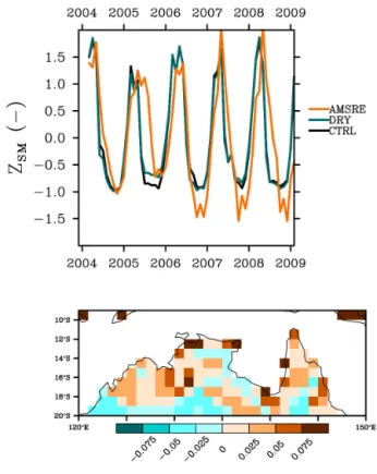
Figure 2. (a)The mean normalized (using the first two moments) first layer soil moisture (SM1) from the CTRL and DRY simula-tions and the AMSR-E observasimula-tions. (b) The difference between the mean SM1(from all simulations over all months from 2004 to 2009) and the AMSR-E observations.
of the simulated moistening. The mean monthly soil mois-ture closely follows the observationally based estimates and exhibits dynamic behavior independent of the model config-uration.
The bias of the ensemble-mean-time-averaged surface layer soil moisture from the eight simulations against the AMSR-E product is shown in Fig. 2b. Over large re-gions of northern Australia, the simulated SM1 is within 0.025 mm3mm−3of AMSR-E. The difference in mean SM1 between the two model configurations is similarly small (fig-ure not shown). Fig(fig-ure 2 demonstrates that the temporal evo-lution (Fig. 2a) and mean state (Fig. 2b) of the simulated SM1 are similar to the AMSR-E estimates.
The seasonal mean ET is validated against the arithmetic mean of the three gridded ET products for both DJF (Fig. 3a, c, e) and SON (Fig. 3b, d, f). The observed DJF ET (Fig. 3e) has a strong north–south gradient with a maxima centered around 13◦S, 130◦E. The strong north–south gradient is also present in the ensemble mean ET (Fig. 3a); however, the simulations overestimate DJF ET over much of the do-main. The observationally based estimates show an ET of less than 50 W m−2south of 18◦S while the simulations re-main above 60 W m−2in this region. The mean SON ET is markedly lower compared to DJF ET in both the gridded data
(Fig. 3f) and the simulations (Fig. 3b). Similar to DJF, both the model and the ET product show a strong north–south gradient. The simulations underestimate the ET in the York Peninsula (east of 140◦E and north of 17◦S) during SON and overestimate the ET in this region during DJF. The overesti-mation of DJF ET compared to the gridded product is much more pronounced for the CTRL simulations (Fig. 3a) than for the DRY simulations (Fig. 3c). The underestimation of the SON ET in the simulations is largely a result of including the DRY model configuration. The CTRL simulations exhibit a 10–20 W m−2increase in SON ET over the DRY model runs (Fig. 3b, d). Overall, the model exhibits spatiotemporal ET in close agreement with this gridded ET product.
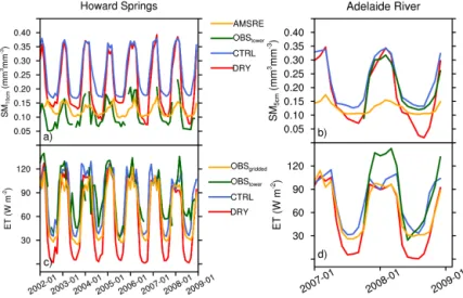
Point measurements of SM and ET at two locations show reasonable agreement with the model simulations. The Howard Springs SM observations 10 cm depth (Fig. 4a) typ-ically increases from 0.05 to 0.2 mm3mm−3from the dry to the wet season. The observations are drier during the wet sea-son and have a smaller (by a factor of 2) seasea-sonal cycle than both the DRY and CTRL simulations. DRY is much drier (∼0.08 mm3mm−3) than CTRL (∼0.18 mm3mm−3) during the dry season and in better agreement with the measure-ments (∼0.05 mm3mm−3). This contrasts with the agree-ment at the Adelaide River site (Fig. 4b) where the mea-surements and CTRL peak at around 0.30 mm3mm−3during the 2008 wet season. DRY (0.02–0.07 mm3mm−3) is again much drier than CTRL (0.15 mm3mm−3) during the 2008 dry season but CTRL is in better agreement with the data (0.15 mm3mm−3). The AMSR-E estimate, CTRL, and DRY are similar in Fig. 4a and b (they axis scale is the same in both figures), while the SM observations at the two sites dif-fer drastically. The disagreement in the mean as well as the amplitude of the seasonal variability is likely due to both the difference in scale between the measurements and simula-tions and poor representation of soil properties in the model. When the SM comparison is normalized using the first two moments as in Fig. 2a (not shown) there is greater agreement between the measurements, AMSR-E, and the simulations.
The ET data at Howard Springs (Fig. 4c) demonstrates that the CTRL simulation always produces too little ET during the dry season. While the gridded ET estimate in Fig. 4c falls within 10 Wm−2of the CTRL simulation during the dry sea-son, the tower data are nearly 20 W m−2greater than during both the 2007 and 2008 dry seasons. The wet season peak in ET is well simulated by both CTRL and DRY at Howard Springs. The model performance is different at the Adelaide River as both CTRL and DRY have a wet season peak ET of around 120 W m−2while the measurements peak closer to 150 W m−2. Figure 4d further demonstrates that DRY has too little dry season ET.
Figure 3.The mean ET (Wm−2) from the wet season (DJF shown in the left hand column) and the transition between the dry and wet seasons (SON shown in the right hand column). The ensemble mean ET from(a)CTRL over DJF,(b)CTRL over SON,(c)DRY for DJF,
(d)DRY from SON,(e)OBS (the mean of three gridded ET products) over DJF, and(f)OBS for SON.
Figure 4.The monthly soil moisture (SM in mm3mm−3) from the ensemble mean from CTRL and DRY, AMSR-E, and flux tower mea-surements (OBStower) from flux tower sites at(a)Howard Springs at 10 cm depth and(b) Adelaide River at 5 cm depth. The monthly
evapotranspiration (ET in Wm−2) from CTRL, DRY, the mean of three ET products (OBSgridded) and the measurements at the(c)Howard
Springs and(d)Adelaide River flux tower sites.
spatial and temporal patterns of ET and SM are generally captured by the modeling system. The accuracy of the es-timated land surface states and fluxes therefore enables the use of the simulated variables in the diagnoses of the land– atmosphere association strength during SON and DJF.
4.2 Background SM state
Figure 5.Spatiotemporal mean soil moisture (mm3mm−3) SM as a function of depth (m) for(a)DJF and(b)SON.
3 m. In contrast, DRY has a peak soil moisture of only ∼0.24 mm3mm−3 at the surface and decreases with depth to near zero at 3 m. Similar patterns of SM with depth are seen over SON; however, SM1is considerably lower for both CTRL and DRY compared to DJF.
Despite the similar mean and temporal behavior of SM1 shown in Fig. 2, SM away from the surface differs substan-tially between the two model configurations (Fig. 5). The mean DJF ET is similar between CTRL and DRY, with dif-ferences between the two of only 10–20 W m−2, correspond-ing to roughly 10–20 % of the mean value. The fractional contribution of transpiration to the total ET during DJF is roughly 10–30 % for both DRY and CTRL (Fig. 6), indi-cating that the evaporation is the dominant ET mechanism. The enhanced mean SM in CTRL causes the CTRL ET to be greater than the DRY ET during DJF, yet both compare rea-sonably well to the observationally based estimates (Fig. 3). However, the lack of SM at depths below several centimeters for DRY during SON causes the reduced ET as compared to CTRL during this period. The mean ET during SON is sen-sitive to the mean SM away from the surface, indicating that transpiration significantly contributes to the total ET during this period as can be seen in Fig. 6. The large contribution of transpiration to the total ET in CTRL (Fig. 6b) is facilitated by the moist subsurface soil moisture (Fig. 5b). The reduced root zone SM in DRY leads to an increase in water stress and reduced transpiration, causing both the lower mean ET and transpiration fraction in DRY relative to CTRL. This reduc-tion during SON is large relative to the mean ET during the period (Fig. 3).
4.3 Correspondence: EF–LCL and SM1–LCL
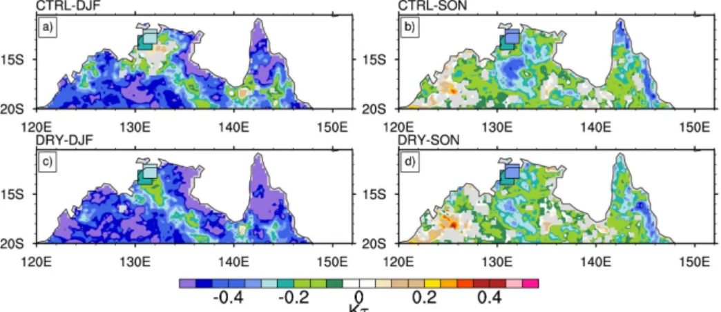
The statistical association between the evaporative fraction and the LCL is shown in Fig. 7, with the results from the two flux towers shown in enclosed squares around 13◦N, 131◦E. The insignificant associations are greyed out while the sta-tistically significant results are shown in color. During DJF, CTRL (Fig. 7a) and DRY (Fig. 7c) exhibit strong surface
flux–atmosphere correspondence, with the strongest associa-tion over the Cape York Peninsula (east of 140◦
E and north of 17◦
S) and the southwestern part of the domain. Similarly, the EF–LCL association is significant during SON (Figs. 7b, d) over much of the domain, although the magnitude is re-duced relative to DJF. Both ensembles show strong associa-tions independent of the season; however, the differences be-tween CTRL and DRY vary with season. The DJF EF–LCL correspondence near 15◦S, 132◦E is statistically significant in DRY (Fig. 7c) but not in CTRL (Fig. 7a), contrasting the similar SON EF–LCL association in this region exhibited by both DRY (Fig. 7d) and CTRL (Fig. 7b). The flux towers (boxed squares in Fig.7a–c) show statistically significant as-sociation between EF and the LCL during both seasons. The EF–LCL correspondence from the tower observations agree more closely with DRY in DJF as CTRL shows statistically insignificant association in the region (13◦
S, 131◦
E). The re-duced deep layer soil moisture resulting from the removal of the groundwater module enhances the DJF correspondence in agreement with the tower data.
Figure 8 shows the medianKτ between SM1and the LCL (see Sect. 3.3) for CTRL and DRY separately during DJF (Fig. 8a, c) and SON (Fig. 8b, d). Several important features are present in Fig. 8. The SM1–LCL association during DJF and SON is largely similar between the two model config-urations. CTRL (Fig. 8a) and DRY (Fig. 8c) exhibit similar spatial patterns and magnitudes ofKτ. Some regions (17◦S, 126◦E) exhibit increases in the magnitude ofKτ in CTRL relative to DRY in DJF (Fig. 8a, c) although the differences are statistically insignificant over most of the domain. Re-gardless of these slight variations inKτ, CTRL and DRY exhibit a strong association between SM1and the boundary layer during the peak of the wet season over coincident parts of the domain. Both model configurations also show areas (15◦S, 131◦E) with insignificant correspondence adjacent to the strongly associated regions. In contrast, CTRL and DRY both contain regions of significant positiveKτ demonstrat-ing a negative correspondence durdemonstrat-ing SON, in disagreement with the results from the Adelaide River tower site. The tower sites show statistically significant negative SM–LCL associ-ation during DJF adjacent to a region (15◦S, 131◦E) of in-significant correspondence in both simulations. The similar-ity in SM1–LCL correspondence between CTRL and DRY during both DJF and SON implies a similar temporal vari-ability of SM1as related to the LCL. From Fig. 3, the mean ET fluxes are considerably different during SON. The simi-lar temporal behavior relative to the LCL for both DRY and CTRL indicates that the SM1 variability is physically inde-pendent of the season’s mean ET fluxes.
Figure 6.The mean transpiration fraction (fraction of total ET from transpiration defined as the ratio of transpiration over total ET) from the wet season (DJF shown in the left hand column) and the transition between the dry and wet seasons (SON shown in the right hand column). The ensemble mean transpiration fraction to total ET from(a)CTRL over DJF,(b)CTRL over SON,(c)DRY over DJF, and(d)DRY over SON.
Figure 7. The ensemble median Kτ correlation metric between the afternoon time (local) EF and the afternoon computed LCL from
(a)CTRL over DJF,(b)CTRL over SON,(c)DRY over DJF, and(d)DRY over SON. The black outlined squares in(a–d)denote the values from the flux tower sites. Only statistically significant (95 % confidence level) results are shown in(a–d).
LCL during DJF and SON in Figs. 7 and 8. The EF–LCL correspondence during DJF is much stronger than the corre-lation from SM1, and DRY exhibits regions of stronger EF– LCL correspondence than CTRL; however, the differences are not statistically significant over much of the domain. A key difference between the flux tower and model simulation estimatedKτis the depth of the SM. The measurement depth at the tower sites are 5 and 10 cm for Adelaide River and Howard Springs respectively, while the model surface layer soil moisture is taken from a depth of 0.7 cm. The change in sign of SM1–LCL Kτ from SON (Fig. 8b, d) to DJF (Fig. 8a, c) demonstrates that applying Eq. (4) to SM1and the LCL does not always capture the co-evolution of the land surface and the atmosphere during periods where deep SM and transpiration dominate the ET flux.
In short, our results demonstrate that the simulated surface layer soil moisture cannot adequately capture the SM–LCL
association during both DJF and SON. The significant con-tributions of transpiration to the total ET fluxes (especially during SON) are responsive to perturbations in SMrzand not SM1.
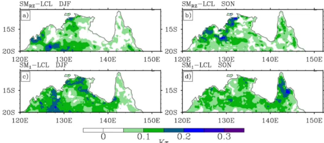
4.4 Proposed Association strength definition: SMrz–LCL
evap-Figure 8.The ensemble medianKτcorrelation metric between the morning first layer soil moisture (SM1) and the afternoon computed LCL
from(a)CTRL over DJF,(b)CTRL over SON,(c)DRY over DJF, and(d)DRY over SON. The black outlined squares in(a–d)denote the values from the flux tower sites. Only statistically significant (95 % confidence level) results are shown in(a–d).
Figure 9.The ensemble medianKτ correlation metric between the morning root zone soil moisture (SMrz) and the afternoon computed
LCL from(a)CTRL over DJF,(b)CTRL over SON,(c)DRY over DJF, and(d)DRY over SON. The black outlined squares in(a–d)denote the values from the Howard Springs flux tower site. Only statistically significant (95 % confidence level) results are shown in(a–d).
oration from the soil. Therefore, the relationship between the temporal variations in SM and the LCL in DJF (or other pe-riods where the ET is largely comprised of soil evaporation) can be adequately defined using SM1. Kτ computed from SM1neglects SMrzvariations that drive transpiration during the initial increase in precipitation following the dry season and therefore may not fully encompass the extent of land– atmosphere associations. Acknowledging the importance of transpiration during the northern Australian wet season, we further evaluate the land–atmosphere association by comput-ingKτ between the vertically averaged SMrzand the LCL. As opposed to remotely sensed SM from AMSR-E (or other satellite products), the use of simulated SM facilitates the es-timation of SMrz. Applying Eq. (4) using SMrzimposes a dif-ferent set of problems, as the rooting depth is model depen-dent and generally only approximately known. There is sub-stantial evidence that eucalypts have rooting depths exceed-ing 20 m (Schenk and Jackson 2002), however neither CLM4 nor the direct observations in this study extend that deep. Due
to these limitations, SMrzis computed as the weighted mean of the SM observations at 10, 40, and 100 cm for the Howard Springs site. We assume that the SMrz consists of the soil layers between the surface and a depth of 1m, as more than 90 % of the prescribed roots in CLM4 are within 1m of the surface (Oleson et al., 2010). This assumed rooting depth is consistent with the model formulation but not realistic given the rooting depths of eucalypts.
Figure 9 shows the ensemble medianKτ diagnosed be-tween SMrz and the LCL. Comparing Figures 8 and 9 it is clear that including the portion of SM that partially controls transpiration increases the magnitude of the DJF SM–LCL associations and eliminates the region near 14◦
Figure 10.The standard deviation of theKτ correlation metric among the ensemble members between the afternoon computed LCL and either the morning root zone soil moisture (SMrz) over(a)DJF and(b)SON or the morning first layer soil moisture (SM1) over(c)DJF and (d)SON.
of insignificant association are prevalent near 13◦ S, 131◦
E. The flux-tower-derived SON SMrz–LCL correspondence is insignificant in agreement with the DRY and CTRL results near 13◦S, 131◦E. The similarity between the DRY and CTRL SMrz–LCL Kτ highlights the negligible groundwa-ter impact (Fig. 9b, d). Comparing Fig. 9b and d with Fig. 3b and d reveals that despite the impact of groundwater on the mean ET flux over SON, the mean state of the deep SM im-parts little influence on the temporal dynamics of SMrz in relation to the LCL. Neglecting the SM beneath the surface layer in the calculation of Kτ results in a weak diagnosis of SM–LCL association during SON because transpiration is partly governed by the water availability within the root zone. By defining the association using SMrz, it is clear that the land is strongly linked to the LCL during both DJF and SON. The DJF SM–LCL association in CTRL near flux tower sites is stronger when defined in this manner, although both sets of simulations still show SMrz to be statistically associated to the LCL.
The SM1–LCL and SMrz–LCLKτ shown in Figs. 8 and 9 are the median from ensembles with 32 estimates. The en-sembles explicitly use multiple constructions of LCL to sam-ple the possible range of atmospheric states given the near-surface MERRA and GLDAS estimates and may lead to un-certain estimates of Kτ. The inter-ensemble uncertainty of theKτ metric is examined to demonstrate the robustness of the results. The standard deviation of the association between SMrzand the LCL and between SM1and the LCL among the ensemble members is generally less than 0.15 (Fig. 10a–d). The variation among the ensemble members is smaller than the median Kτ shown in Figs. 8 and 9. The low standard deviation relative to the median demonstrates that the associ-ation shown in Figs. 8 and 9 is robust, since more than 83 % of theKτestimates (assuming they are normally distributed) have a correspondence of the same sign reported in the fig-ures. The correspondence using SM1(Fig. 10c) shows larger
ensemble uncertainty near the coast centered around 135◦ E compared to the SMrzassociation in DJF (Fig. 10a) and over the Cape York Peninsula in SON (Fig. 10b, a). Aside from the region near 15◦S, 130◦E during SON, the larger ensem-ble uncertainty is found when using SM1to define the corre-spondence.
5 Discussion
The EF–LCL association (Fig. 7) is similar for both model configurations despite the mean ET (Fig. 3), SM (Fig. 5) and transpiration fraction (Fig. 6) differing considerably be-tween CTRL and DRY. The EF–LCL similarity holds for both DJF and SON despite the differing background soil moisture states between the two periods and differing con-tributions of transpiration to the total ET (Fig. 6). The results indicate that while the mean ET and transpiration fraction is a strong function of mean soil moisture, the SM–LCL as-sociation diagnosed using offline simulations of SM and EF with an observationally estimated LCL is insensitive to the background state. The coincidence of the temporal variations in SM, EF, and LCL are demonstrated by the large values of Kτ. These seemingly counterintuitive results may be an artifact of using a rank correlation coefficient to determine the strength of the correspondence. Kτ only measures the temporal coincidence of the two time series while neglecting the magnitude of these variations. Therefore,Kτ cannot dis-tinguish between a dry SM state with the small evaporative fluxes and a wet state with large fluxes if the timing of the SM and flux variations are identical. AlthoughKτ is largely independent to the background soil moisture state, alternative definitions of association may not remain as invariant.
While association in Fig. 7 is largely unaffected by the mean SM state, the mean ET flux is largely derived from deeper SM through transpiration during the onset of the wet season prior to DJF. The statistical relationship between soil moisture and the boundary layer under these conditions is poorly defined using SM1. The consistent EF–LCL co-evolution during SON and DJF highlights the inadequacy of characterizing land–atmosphere processes using only SM1. Attempting to define the SM–LCL relationship with SM1 re-sults in a physically improbable conclusion whereKτ tran-sitions from positive (Fig. 7b) to negative (Fig. 7a) as the wet season is established (Fig. 1) and directly contradicts the EF–LCL results. Despite the domain’s mean precipita-tion increasing from roughly zero to several millimeters per day during SON,Kτ from SM1–LCL is both positive (i.e., 15◦S, 126◦E) and negative (i.e., 15◦S, 134◦E) over this pe-riod. The transition from negligible (or positive) to strong statistical rank correlation between the soil moisture and the atmosphere during the wet season is an artifact resulting from the use of SM1. More consistent correspondence in general agreement with the EF–LCL dynamics throughout the wet season exists between SMrz and LCL because transpiration is incorporated into the diagnostic. During SON, the dry sur-face layer SM is responsible for little ET, so variations in ET are not associated with variations in SM1. The SMrz–LCL Kτ eliminates the insignificant association around 17◦S, 128◦E exhibited in the SM1–LCL metric. Despite regions of significant SMrz–LCL association in DRY and CTRL, the Howard Springs data show insignificant SMrz–LCL corre-spondence during SON. The lack of observed association is possibly related to the inability to sample SM at depths that correspond to the physically relevant rooting depths. The
ne-cessity of using SMRZagrees with Lee et al. (2012), where transpiration was found to limit precipitation variability over tropical regions. The importance of transpiration among the various ET components is not limited to northern Australia or monsoon regions (Coenders-Gerrits et al., 2014; Schlesinger and Jasechko, 2014), highlighting the need to characterize land–atmosphere dynamics using SM well beneath the sur-face.
Statistically determing the association using only near-surface variables from land near-surface model simulations and atmospheric data as done in this study (i.e. Ferguson et al., 2012; Betts, 2009) is limited due to only examining a part of the full land–atmosphere coupling processes. While the LCL is an important determinant in the formation of precipi-tation, moisture convergence, upper level inversions, convec-tive available potential energy, wind shear, and many other factors play important roles in the formation of convection. The correspondence diagnosed in this study with Eq. (4) is by definition limited in scope to only part of the coupling contin-uum described in Eq. (1). Therefore, an association defined using these methods provides a necessary but not sufficient condition for strong land–atmosphere interactions between soil moisture and precipitation.
Our results likely extend to monsoonal regions beyond northern Australia. GLACE (Global Land–Atmosphere Cou-pling Experiment; Koster et al., 2006) revealed multiple ar-eas of strong land–atmosphere coupling coincide with ma-jor monsoon systems. The strong co-evolution during the wet season (September–February) diagnosed using SMrzand Kτ in our results qualitatively agrees with the strong cou-pling in monsoon regions from GLACE. The dry season an-tecedent to the large precipitation fluxes induces low evap-oration while allowing deeply rooted plants to transpire de-spite the prolonged dry period. These conditions over north-ern Australia (Figs. 3, 4) lead to transpiration dominating the ET flux during the onset of the wet season. The behavior of the land–atmosphere system as diagnosed usingKτ under these conditions must be defined using SMrzrather than SM1 to ensure the relevant pathways of the moisture fluxes are not neglected.
6 Conclusions
The feasibility of diagnosing the land–atmosphere relation-ship using a rank correlation coefficient is analyzed utilizing ensembles of land surface simulations and near-surface at-mospheric data. Using four forcing data sets, ensembles of CLM simulations over northern Australia are performed, us-ing configurations that intentionally span a range of mean SM states by either including or neglecting soil column– groundwater interactions. The seasonal dynamics of the sim-ulated SM1is insensitive to the mean soil moisture state and all simulations compare favorably with the AMSR-E soil moisture product. Furthermore, the simulated ET from De-cember to February is similar between the CTRL and DRY runs, with both configurations largely consistent with the DJF ET estimated from three gridded ET products.
The strength of the temporal co-evolution of land and at-mosphere states is diagnosed between both SM1and EF from the simulations and the LCL as calculated from the near-surface atmospheric data. In line with the coupling strength found in previous studies, during the peak wet season strong SM1–LCL and EF–LCL associations are shown. The wet season onset (SON) shows large rank correlation coefficients between EF and LCL that contrasts the lack of correlation between SM1 and LCL. The contradicting correlations be-tween EF–LCL and SM1–LCL demonstrate that the SON land–atmosphere relationship is not properly characterized with SM1. The land–atmosphere interactions during periods with non-negligible transpiration necessitates the use of root zone soil moisture instead of the surface soil moisture to properly capture the physical processes. The correlation be-tween SMrzand LCL differs considerably from that between SM1and LCL. The co-evolution of SMrzand LCL is shown by strong statistical correspondence throughout the wet sea-son and is consistent with the co-evolution between EF and LCL. During the peak of the wet season, SM1is sufficient to explain the SM–LCL association while during the monsoon season onset SMrzis necessary. The results demonstrate that the root zone soil moisture must be considered when diag-nosing the relationship between SM and the LCL.
Our results show that the statistically diagnosed land– atmosphere correspondence in offline simulations is insen-sitive to the mean vertical profile of soil moisture. It is, however, sensitive to the depth of the soil moisture con-sidered. While the strong soil moisture-atmosphere associ-ations shown here are a necessary but not sufficient con-dition to diagnose full land–atmosphere coupling, the re-sults demonstrate the need to describe SM–LCL coupling using the physically relevant soil moisture. Studies that ex-plore the behavior of the land–atmosphere system should use a statistical measure which encapsulates the SM that is physically relevant to the dominant processes. Future stud-ies that evaluate land–atmosphere coupling using a full land– atmosphere model environment risk not capturing regions of land–atmosphere coupling if only SM1is considered. In
or-der to evaluate coupling during periods when ET is domi-nated by transpiration, SMrz should be considered. We rec-ommend that future studies of land–atmosphere coupling fo-cus on root zone soil moisture rather than surface layer soil moisture.
Acknowledgements. We acknowledge support from the Australian Research Council Super Science scheme (FS100100054). A. J. Pitman was also supported by the Australian Research Council Centre of Excellence for Climate System Science (CE110001028). J. P. Evans was supported by an Australian Research Council Future Fellowship (FT110100576). The GLDAS data used in this study were acquired as part of the NASA’s Earth-Sun System Division and archived and distributed by the Goddard Earth Sciences (GES) Data and Information Services Center (DISC) Distributed Active Archive Center (DAAC). We also thank Diego Miralles for providing the GLEAM ET product.
Edited by: P. Gentine
References
Betts, A. K.: Land-surface-atmosphere coupling in observa-tions and models, J. Adv. Model. Earth Syst., 1, 4, doi:10.3894/JAMES.2009.1.4, 2009.
Betts, A. K., Ball, J. H., Beljaars, A. C. M., Miller, M. J., and Viterbo, P. A.: The land surface-atmosphere interaction: a review based on observational and global modeling perspectives, J. Geo-phys. Res., 101, 7209–7225, doi:10.1029/95JD02135, 1996. Betts, A. K., Helliker, B., and Berry, J.: Coupling between CO2,
water vapor, temperature, and radon and their fluxes in an ide-alized equilibrium boundary layer over land, J. Geophys. Res., 109, 7209–7225, doi:10.1029/2003JD004420, 2004.
Beringer, J.: Adelaide River OzFlux tower site, OzFlux: Aus-tralian and New Zealand Flux Research and Monitoring, hdl:102.100.100/14228, CSIRO, Dickson, Australia, 2013a. Beringer, J.: Howard Springs OzFlux tower site, OzFlux:
Aus-tralian and New Zealand Flux Research and Monitoring, hdl:102.100.100/14234, CSIRO, Dickson, Australia, 2013b. Bosilovich, M. G., Chen, J., Robertson, F. R., and Adler, R. F.:
Eval-uation of global precipitation in reanalyses, J. Appl. Meteorol. Clim., 47, 2279–2299, 2008.
Coenders-Gerrits, A. M. J., van der Ent, R. J., Bogaard, T. A., Wang-Erlandsson, L., Hrachowitz, M., and Savenije, H. H. G.: Uncertainties in transpiration estimates, Nature, 506, doi:10.1038/nature12925, 2014.
Decker, M., Pitman, A., and Evans, J. P.: Groundwater constraints on simulated transpiration variability over Southeastern Aus-tralian forests, J. Hydrometeorol., 14, 543–559, 2013.
Draper, C. S., Walker, J. P., Steinle, P. J., de Jeu, R. A. M., and Holmes, T. R. H.: An evaluation of AMSR-E derived soil mois-ture over Australia, Remote Sens. Environ., 113, 703–710, 2009. Evans, J. P., Pitman, A. J., and Cruz, F. T.: Coupled atmospheric and land surface dynamics over southeast Australia: a review, analy-sis and identification of future research priorities, Int. J. Clima-tol., 31, 1758–1772, doi:10.1002/joc.2206, 2011.
Ferguson, C. R. and Wood, E. F.: Observing land–atmosphere inter-action globally with satellite remote sensing, in: Proc. Earth Ob-servation and Water Cycle Science Symp., Frascati, Italy, edited by: Lacoste, H., ESA Publications Division, European Space Agency, Noordwijk, The Netherlands, 8 pp., 2009.
Ferguson, C. R., Wood, E. F., and Vinukollu, R. K.: A global in-tercomparison of modeled and observed land–atmosphere cou-pling, J. Hydrometeorol., 13, 749–784, doi:10.1175/JHM-D-11-0119.1, 2012.
Gentine, P., Entekhabi, D., and Polcher, J.: The diurnal behavior of evaporative fraction in the soil–vegetation–atmospheric bound-ary layer continuum, J. Hydrometeorol., 12, 1530–1546, 2011. Gentine, P., Ferguson, C. R., and Holtslag, A. A. M.:
Di-agnosing evaporative fraction over land from boundary-layer clouds, J. Geophys. Res.-Atmos., 118, 8185–8196, doi:10.1002/jgrd.50416, 2013a.
Gentine, P., Holtslag, A. A. M., D’Andrea, F., and Ek, M.: Sur-face and Atmospheric Controls on the Onset of Moist Convection over Land, J. Hydrometeorol., 14, 1443–1462, 2013b.
Guo, Z., Dirmeyer, P. A., Koster, R. D., Bonan, G., Chan, E., Cox, P., Gordon, C. T., Kanae, S., Kowalczyk, E., Lawrence, D., Liu, P., Lu, C.-H., Malyshev, S., Mcavaney, B., Mcgregor, J. L., Mitchell, K., Mocko, D., Oki, T., Oleson, K. W., Pitman, A., Sud, Y. C., Taylor, C. M., Verseghy, D., Vasic, R., Xue, Y., and Yamada, T.: GLACE: the global land–atmosphere coupling experiment. Part II: Analysis, J. Hydrometeorol., 7, 611–625, doi:10.1175/JHM511.1, 2006.
Hirsch, A., Kala, J., Pitman, A. J., Carouge, C., Evans, J. P., Haverd, V., and Mocko, D.: Impact of land surface initialisation approach on sub-seasonal forecast skill: a regional analysis in the Southern Hemisphere, J. Hydrometeorol., 15, 300–319, 2014.
Huffman, G. J., Bolvin, D. T., Nelkin, E. J., Wolff, D. B., Adler, R. F., Gu, G., Hong, Y., Bowman, K. P., and Stocker, E. F.: The TRMM Multisatellite Precipitation Analysis (TMPA): quasi-global, multiyear, combined-sensor precipitation estimates at fine scales, J. Hydrometeorol., 8, 38–55, doi:10.1175/JHM560.1, 2007.
Jiménez, C., Prigent, C., Mueller, B., Seneviratne, S. I., Mc-Cabe, M. F., Wood, E. F., Rossow, W. B., Balsamo, G., Betts, A. K., Dirmeyer, P. A., Fisher, J. B., Jung, M., Kanamitsu, M., Reichle, R. H., Reichstein, M., Rodell, M., Sheffield, J., Tu, K., and Wang, K.: Global intercomparison of 12 land surface heat flux estimates, J. Geophys. Res., 116, D02102, doi:10.1029/2010JD014545, 2011.
Jones, D. A., Wang, W., and Fawcett, R.: High-quality spatial cli-mate data-sets for Australia, J. Aust. Meteor. Oceanogr., 58, 233– 248, 2009.
Jung, M., Reichstein, M., Ciais, P., Seneviratne, S. I., Sheffield, J., Goulden, M. L., Bonan, G., Cescatti, A., Chen, J., de Jeu, R., Dolman, A. J., Eugster, W., Gerten, D., Gianelle, D., Go-bron, N., Heinke, J., Kimball, J., Law, B. E., Montagnani, L., Mu, Q., Mueller, B., Oleson, K., Papale, D.,
Richard-son, A. D., Roupsard, O., Running, S., Tomelleri, E., Viovy, N., Weber, U., Williams, C., Wood, E., Zaehle, S., and Zhang, K.: Recent decline in the global land evapotranspira-tion trend due to limited moisture supply, Nature, 467, 951–954, doi:10.1038/nature09396, 2010.
Koster, R. D. and Suarez, M. J.: Impact of land surface initialization on seasonal precipitation and temperature prediction, J. Hydrom-eteorol., 4, 408–423, 2003.
Koster, R. D., Suarez, M. J., Higgins, R. W., and Van den Dool, H. M.: Observational evidence that soil moisture vari-ations affect precipitation, Geophys. Res. Lett., 30, 1241, doi:10.1029/2002GL016571, 2003.
Koster, R. D., Suarez, M. J., and Heiser, M.: Variance and pre-dictability of precipitation at seasonal-to-interannual timescales, J. Hydrometeorol., 1, 26–46, 2000.
Koster, R. D., Guo, Z., Dirmeyer, P. A., Bonan, G., Chan, E., Cox, P., Davies, H., Gordon, C. T., Kanae, S., Kowalczyk, E., Lawrence, D., Liu, P., Lu, C.-H., Malyshev, S., Mcavaney, B., Mitchell, K., Mocko, D., Oki, T., Oleson, K. W., Pitman, A., Sud, Y. C., Taylor, C. M., Verseghy, D., Vasic, R., Xue, Y., and Ya-mada, T.: GLACE: the global land–atmosphere coupling experi-ment, Part I: Overview, J. Hydrometeorol., 7, 590–610, 2006. Koster, R. D., Z., Guo, R., Yang, P. A., Dirmeyer, K., Mitchell, and
Puma, M. J.: On the Nature of Soil Moisture in Land Surface Models, J. Climate, 22, 4322–4335, 2009.
Koster, R. D., Mahanama, S. P. P., Yamada, T. J., Balsamo, Gian-paolo, Berg, A. A., Boisserie, M., Dirmeyer, P. A., Doblas-Reyes, F. J., Drewitt, G., Gordon, C. T., Guo, Z., Jeong, J.-H., Lee, W.-S., Li, Z., Luo, L., Malyshev, S., Merryfield, W. J., Seneviratne, S. I., Stanelle, T., van den Hurk, B. J. J. M., Vitart, F., and Wood, E. F.: The second phase of the global land–atmosphere coupling exper-iment: soil moisture contributions to subseasonal forecast skill, J. Hydrometeorol., 12, 805–822, doi:10.1175/2011JHM1365.1, 2011.
Lee, J.-E., Lintner, B., Neelin, J. D., Jiang, X., Gentine, P., Boyce, C. K., Fisher, J. B., Perron, J. T., Kubar, T. L., Lee, J., and Worden, J. R.: Reduction of tropical land region precipitation variability via transpiration, Geophys. Res. Lett., 39, L19704, doi:10.1029/2012GL053417, 2012.
Lintner, B. R. and Neelin, J. D.: Soil moisture impacts on convective margins, J. Hydrometeorol., 10, 1026–1039, 2009.
Lintner, B. R., Gentine, P., Findell, K. L., D’Andrea, F., Sobel, A. H., and Salvucci, G. D.: An idealized prototype for large-scale land–atmosphere coupling, J. Climate, 26, 2379–2389, 2013. Liu, Y. Y., van Dijk, A. I. J. M., De Jeu, R. A. M., and Holmes,
T. R. H.: An analysis of spatiotemporal variations of soil and vegetation moisture from a 29-year satellite-derived data set over mainland Australia, Water Resour. Res., 45, W07405, doi:10.1029/2008WR007187, 2009.
Meng, X. H., Evans, J. P., and McCabe, M. F.: The impact of ob-served vegetation changes on land–atmosphere feedbacks during drought, J. Hydrometeorol., 15, 759–776, doi:10.1175/JHM-D-13-0130.1, 2014a.
Meng, X. H., Evans, J. P., and McCabe, M. F.: The influence of inter-annually varying albedo on regional climate and drought, Clim. Dynam., 42, 787–803, doi:10.1007/s00382-013-1790-0, 2014b.
its components at the global scale, Hydrol. Earth Syst. Sci., 15, 967–981, doi:10.5194/hess-15-967-2011, 2011a.
Miralles, D. G., Holmes, T. R. H., De Jeu, R. A. M., Gash, J. H., Meesters, A. G. C. A., and Dolman, A. J.: Global land-surface evaporation estimated from satellite-based observations, Hydrol. Earth Syst. Sci., 15, 453–469, doi:10.5194/hess-15-453-2011, 2011b.
Mu, Q., Heinsch, F. A., Zhao, M., and Running, S. W.: Development of a global evapotranspiration algorithm based on MODIS and global meteorology data, Remote Sens. Environ., 111, 519–536, doi:10.1016/j.rse.2007.04.015, 2007.
Mu, Q., Zhao, M., and Running, S. W.: Improvements to a MODIS global terrestrial evapotranspiration algorithm, Remote Sens. En-viron., 115, 1781–1800, doi:10.1016/j.rse.2011.02.019, 2011. Njoku, E. G., Jackson, T. J., Lakshmi, V., Chan, T. K., and Nghiem,
S. V.: Soil moisture retrieval from AMSR-E, IEEE T. Geosci. Remote, 41, 215–229, doi:10.1109/TGRS.2002.808243, 2003. Oleson, K. W., Lawrence, D. M., Bonan, G. B., Flanner, M. G.,
Kluzek, E., Lawrence, P. J., Levis, S., Swenson, S. C., Thornton, P. E., Dai, A., Decker, M., Dickinson, R., Feddema, J., Heald, C. L., Hoffman, F., Lamarque, J.-F., Mahowald, N., Niu, G.-Y., Qian, T., Randerson, J., Running, S., Sakaguchi, K., Slater, A., Stöckli, R., Wang, A., Yang, Z.-L., Zeng, X., and Zeng, X.: Tech-nical Description of Version 4.0 of the Community Land Model (CLM), National Center for Atmospheric Research (NCAR), Boulder, Colorado, doi:10.5065/D6FB50WZ, 2010.
Pielke, R. A., Pitman, A., Niyogi, D., Mahmood, R., McAlpine, C., Hossain, F., Goldewijk, K. K., Nair, U., Betts, R., Fall, S., Re-ichstein, M., Kabat, P., and de Noblet, N.: Land use/land cover changes and climate: modeling analysis and observational evi-dence, WIREs Clim. Change, 2, 828–850, doi:10.1002/wcc.144, 2011.
Pitman, A. J.: The evolution of, and revolution in, land surface schemes designed for climate models, Int. J. Climatol., 23, 479– 510, doi:10.1002/joc.893, 2003.
Press, W. H., Flannery, B. P., Teukolsky, S. A., and Vetterling, W. T.: Nonparametric or rank correlation, numerical recipes, in: C: the Art of Scientific Computing, 2nd Edn., edited by: Cowles, L. and Harvey, A., Cambridge University Press, UK, 639–644, 1992.
Qian, T., Dai, A., Trenberth, K. E., and Oleson, K. W.: Simula-tion of global land surface condiSimula-tions from 1948 to 2004, Part I: Forcing data and evaluations, J. Hydrometeorol., 7, 953–975, doi:10.1175/JHM540.1, 2006.
Rodell, M., Houser, P. R., Jambor, U., Gottschalck, J., Mitchell, K., Meng, C.-J., Arsenault, K., Cosgrove, B., Radakovich, J., Bosilovich, M., Entin, J. K., Walker, J. P., Lohmann, D., and Toll, D.: The global land data assimilation system, B. Am. Meteorol. Soc., 85, 381–394, doi:10.1175/BAMS-85-3-381, 2004. Santanello, J. A., Peters-Lidard, C. D., and Kumar, S. V.:
Diag-nosing the sensitivity of local land–atmosphere coupling via the soil moisture-boundary layer interaction, J. Hydrometeorol., 12, 766–786, doi:10.1175/JHM-D-10-05014.1, 2011.
Schenk, H. J. and Jackson, R. B.: The Global Biogeography of Roots, Ecol. Monogr., 73, 311–328, 2002.
Schlesinger, W. H. and Jasechko, S.: Transpiration in the global water cycle, Agr. Forest Meteorol., 189–190, 115–117, doi:10.1016/j.agrformet.2014.01.011, 2014.
Seneviratne, S. I., Corti, T., Davin, E. L., Hirschi, M., Jaeger, E. B., Lehner, I., Orlowsky, B., and Teuling, A. J.: Investigating soil moisture-climate interactions in a changing climate: a review, Earth-Sci. Rev., 99, 125–161, doi:10.1016/j.earscirev.2010.02.004, 2010.
Taylor, C. M. and Ellis, R. J.: Satellite detection of soil moisture impacts on convection at the mesoscale, Geophys. Res. Lett., 33, L03404, doi:10.1029/2005GL025252, 2006.
Westra, D., Steeneveld, G. J., and Holstag, A. A. M.: Some obser-vational evidence for dry soils supporting enhanced relative hu-midity at the convective boundary layer top, J. Hydrometeorol., 13, 1347–1358, 2012.
Williams, J. L. and Maxwell, R. M.: Propagating subsur-face uncertainty to the atmosphere using fully coupled stochastic simulations, J. Hydrometeorol., 12, 690–701, doi:10.1175/2011JHM1363.1, 2011.