Improving Blood Flow Simulations Using Known Data
T. Guerra
*1and J. Tiago
21
Instituto Politécnico de Setúbal, Centro de Matemática e Aplicações da Faculdade de Ciências e
Tecnologia da Universidade Nova de Lisboa,
2Centro de Matemática e Aplicações, Instituto
Superior Técnico, Universidade de Lisboa.
*Rua Américo da Silva Marinho, Barreiro, 2839-001, Lavradio, Portugal, [email protected]
Abstract: Numerical simulations applied to blood flow together with the imaging processing advances are a powerful tool in the prevention and treatment of some diseases. The inclusion of real data in the numerical blood flow simulations allows the achievement of more realistic and accurate results. In the literature, these techniques are known as Data Assimilation (DA) techniques. In this work we solve a variational DA problem to numerically reconstruct the blood flow circulation inside a real artery, deformed by a saccular aneurysm obtained from medical images and then imported to COMSOL Multiphysics®. We propose a weighted cost function that accurately recovers both the velocity and the wall shear stress profiles. The robustness of such cost function is tested with respect to different velocity inlet profiles. Keywords: Data Assimilation, Optimal Control, Numerical Simulations.
1. Introduction
In this paper we propose a Data Assimilation procedure, which consists in solving an optimal control problem to numerically reconstruct the blood flow in a realistic saccular aneurysm. This can be understood as a preliminary step, before including real data measurements in the simulations, which will allow to build a tool in order to be available to the medical community, contributing to the advancement in therapy prediction, training and expenses reduction.
In the DA method we take into account the wall shear stress (wss), once it can be a measure associated to disturbed flow (see [1,7]), and we verify that this leads to a better precision in a posteriori measurements. We validate the robustness of the method with respect to different flow profiles. In this paper we model the blood flow as an incompressible and laminar
momentum and the conservation of angular momentum.
We propose a non-typical cost functional (1), which, besides the velocity and a regularization term for the control, also includes the wss data information. This technique was already tested in [8] for blood flow assuming a non-Newtonian behavior in 2D idealized geometries.
This paper is organized as follows: first, in section 2, we describe the control problem including the blood flow modeling equations, the viscosity model, the physiological parameters used and the criterion to attain. In section 3 we address the numerical approach while its implementation using COMSOL Multiphysics® is described in section 4. The numerical results related with the robustness and the efficiency of the proposed method, are presented in section 5. Finally, in section 6, we outline the conclusions about the reached results.
2. Problem Description
The main goal is to obtain a numerical solution in a realistic domain Ω, which coincides with available data measured in certain parts of the domain Ωpart, within a predefined error.
We define an optimal control problem using a criterion according to our interests. In this work the criterion chosen is defined by the following cost functional: Min J (u,h) = w1 | u - ud|2dx + Ω part
∫
+ w2 | ws - wsd |2dx Γwall∫
+ w3 | ∇ h |2 dx. (1) Ωin∫
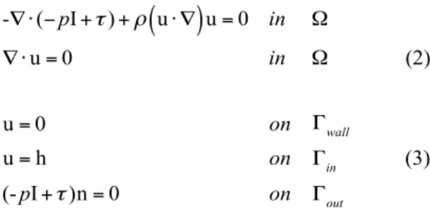
Taking account the non-Newtonian viscosity behavior for the blood flow, the usual modeling system takes the form:
-∇ ⋅ (− pI +τ ) + ρ u ⋅ ∇
(
)
u = 0 in Ω ∇ ⋅ u = 0 in Ω (2) u = 0 on Γwall u = h on Γin (3) (- pI +τ )n = 0 on Γout Here the domain Ω represents the lumen inside an artery that has been deformed by an aneurysm. The lumen is truncated by two planar surfaces. We call the proximal surface by Γin and the distal one by Γout. The interface of the lumen with artery wall is represented by Γwall These surfaces are represented in Figure 1.The cost function essentially measures the misfit between the data and the solution at several sections, Ωpart, as shown in Figure 1.
Figure 1. Computational domain Ω; subset Ωpart;
boundaries representation.
The misfit considers the velocity field, represented by the variable u and wall shear stress magnitude measurements, represented by
ws, and whose expression can be written as it
follows ws = wss,wss = = µ!∇u + ∇u
( )
T " # $ %&n −µ !∇u + ∇u
( )
T " # $ % &n ! " # $ % &n ' ( ) * + ,nwhere n is the outward normal vector to the wall surface. We include the ws since it is an important indicator to predict vascular diseases, which is highly sensitive with respect to the geometry. We also include a regularizing term for the control function, h, to avoid numerical spurious minima, as suggested in [3]. The control function, h, corresponds to the velocity profile at the inlet boundary and p stands for the pressure.
The variables ud and wsd represent the data for the velocity and wall shear stress magnitude registered in Ωpart and in Γwall respectively. The constants w1, w2, w3 are the parameters of the cost functional terms. Concerning system (2), the variable τ represents the extra stress tensor given by τ= 2µ(| Du |)Du, where Du =∇u + ∇u
( )
T 2 .The viscosity µ is defined using the non-Newtonian Carreau model
µ(γ ) = µ∞+ (µ0−µ∞) µ0−µ∞ 1+ (λγ )2
(
)
1−n2 , with γ= 2Du : Du .The parameters considered for the viscosity model (see [1]) are given by
µ∞= 0.0032 Pa.s; µ0= 0.0456 Pa.s; ρ=1050 kg/m 3 λ = 10.03 s; n = 0.344.
For the boundary conditions we use the typical conditions in Hemodynamical problems. Therefore, in (3) we impose no slip conditions on the wall and Neumann homogeneous at the outlet.
At this preliminary stage we will not use real data ud and wsd but rather generate it by solving the forward problem (2). To this end, we use the boundary conditions (3) and we set h to be the parabolic Poiseuille profile defined by
z =U0 1− x R " # $ % & ' 2 + y R " # $ % & ' 2 " # $ $ % & ' '.
Here U0 = 0.419507 represents the maximum velocity and R is the inlet radius. The data generated as described above is included in the cost functional (1) and the control problem is then solved.
3. Numerical Approach
In this work we obtain the numerical solution by the Discretize then Optimize (DO) approach since it seems to be better in Hemodynamical problems when compared with Optimize then Discretize (OD) (see [4]). The DO approach consists in first discretizing the optimal control problem and then solve the finite dimensional optimization problem resulting from the discretization. We can then use the typical Finite Elements Method, and choose the appropriate finite dimensional spaces, for the unknowns and test functions, so that the existence of an approximated solution for problem (2) can be ensured (see [5]).
The discretized problem can be expressed by Min J (u,h) = w1U −Ud N
u 2 + w2W (U ) + w3 H Nh 2 s.a. Q(U ) +G(U )U + BTP = F BU = 0 " # $ %$
where ||.||Nu and ||.||Nh are the resulting norms of the discretization and U=(Uh, H) includes the controlled velocity coefficients H and the uncontrolled ones, represented by Uh =Uh(H).
4. Use of COMSOL Multiphysics
We use COMSOL Multiphysics® to model the blood flow considering a generalized stationary Navier-Stokes system. The geometry representing the real artery is obtained from medical images and imported to COMSOL Multiphysics®. As already mentioned, the data to be used in the DA process is generated by solving the forward problem, with realistic parameters and boundary conditions. We then use the Optimization Module to define a cost function to be minimized.
To solve the discretized problem which is nonlinear both with respect to the cost function and constraints we use the package Sparse Nonlinear Optimization (SNOPT) available in the Optimization Module of COMSOL Multiphysics® (see [6, 9, 10] for more details).
To discretize the control variable we consider quadratic shape functions of the Lagrange type. The cost function is implemented through the Global Objective entry of the Optimization interface. We use the Cholesky QP solver to solve each linear quadratic problem, until the optimality conditions are fulfilled, within a tolerance of 10-6.
The blood flow model (2) is implemented using the Laminar Flow interface, where the viscosity law is introduced explicitly. For the discretization we use P1-P1 finite elements with streamline and crosswind diffusion stabilization. Then a physics based mesh, composed by tetrahedral and quadrilateral elements, corresponding to 180789 degrees of freedom for the velocity variables, is built. The nonlinear problem is treated with Newton’s method by using the direct solver PARDISO to solve each resulting linear system.
5. Numerical Results
The inlet surface Γin can be approximated by a circle with radius R=2.71015 mm. Hence the dimensionless Reynolds number associated to the entering flow is Rey=373, which is a physiological value.
The results for velocity field solution of the forward problem can be observed on Figure 2. There the velocity vectors at the inlet and on , are represented. We will use the later to
obtain ud and wsd as representatives of the true solution that we want to recover accurately.
Figure 2. Velocity field profile for the forward problem.
5.1 Flow reconstruction using DA
Next, the control problem is solved using the
cost function parameters
w1,w2,w3
(
)
= 102,102,10−3(
)
. We compare theresults obtained with the forward problem with those obtained with the control problem. The Figure 3 illustrates the controlled velocity profile throughout the geometry and Figure 4 is an expansion of the saccular region highlighting a strong flow recirculation inside it, according to our expectations.
Figure 3. Velocity field profile for the control problem.
Figure 4. Flow recirculation inside the saccular region.
The Figure 5 represents the contour of the wall shear stress magnitude, taking the red color to high stress and dark blue to low stress. Clearly, within the aneurysm the wall shear stress is lower and the highest values occurs in the biggest curvature between the saccular region and the vessel.
Figure 5. Contour of the wall shear stress magnitude
inside the saccular region.
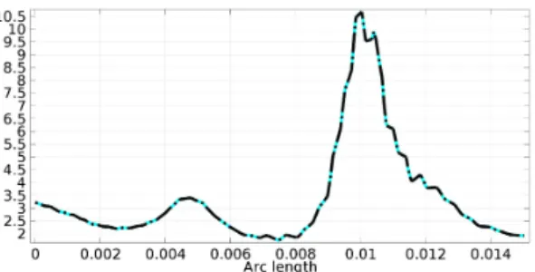
We measure the wall shear stress magnitude along a surface line passing through curvature where the stress is greatest and the result can be viewed in the following line graph, in Figure 6, where the highest value corresponds to the red region observed in Figure 5.
Figure 6. Wall shear stress magnitude as a function of
arc length. Solid Cyan: pretended wss; black dash-dot: controlled wss.
5.2 Testing with different ud and wsd profiles
In order to prove the robustness of the proposed method, we test it with different data. For this purpose we generate two different “true” solutions corresponding to the inlet profiles given by z =U0 1− x2 + y2 R " # $ $ % & ' ' ξ " # $ $ $ % & ' ' '
for ξ=4 and ξ=9. The last one is commonly used in the numerical simulations of blood flow in arteries (see [2]). Note that for ξ=2 we have the Poiseuille (parabolic) profile.
We compared the results of the control problem with the data measurements, in the three tested cases, computing a relative error between u and ud given by Re = | u - ud |2 Ω
∫
dx ! " ## $ % && | ud|2dx Ω∫
# $ %% & ' (( 1/2 1/2 .Those comparisons may be viewed in the following Table 1:
Table 1:Relative Errors for the different data inlet profiles.
Profiles ξ=2 ξ=4 ξ=9
Re 0.002066 0.003636 0.004843
Cost 0.001735 0.006242 0.012496
We can see that even if in the parabolic case the method performs better, the cost function is minimized and the errors are accurate in all of the tree cases.
As already mentioned the control variable at the inlet plays the role of reproducing the inlet profile. In Figure 7 we can compare the inlet profiles used to generate data with the computed control. We can observe an almost perfect adjustment in the case ξ=2. The adjustment becomes less precise for ξ=4 and ξ=9, which is consistent with the conclusions of the Table 1.
Figure 7. Solid grey: pretended inlet profiles; color wireframe: computed controls. Left to right: parabolic (ξ=2), semi-flat (ξ=4) and flat (ξ=9) profiles.
In order to emphasize the wss significance in the proposed cost functional we solved the problem (1), (2) e (3) replacing the cost functional (1) by the following one
Min J (u,h) = w1 | u - ud| 2 dx + Ω part
∫
w3 | ∇ h |2dx Ωin∫
where we take w2=0, ie, not considering the term corresponding to the wall shear stress.
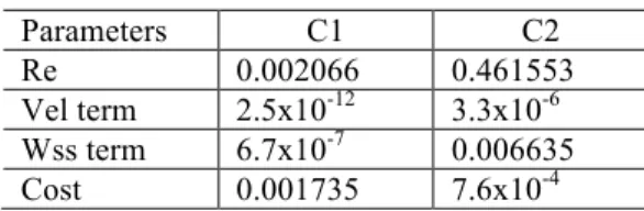
Generating data with the parabolic inlet profile and solving the control problem, we confirm that the presence of this term is important to have a better precision in the results achieved. Both the velocity and the wss are better approximated when all the parameters are not null. These conclusions can be confirmed with the results shown in Table 2, where C1 corresponds to the case (102, 102, 10-3) and C2 to (102, 0, 10-3). Vel term corresponds to the velocity term and Wss term to the wall shear stress term in the cost functional.
Table 2: Relative errors and values for the cost functional terms. Parameters C1 C2 Re 0.002066 0.461553 Vel term 2.5x10⁻¹² 3.3x10⁻⁶ Wss term 6.7x10⁻⁷ 0.006635 Cost 0.001735 7.6x10⁻⁴
Taking into account the obtained values, a worse approximation is expected for the control data with respect to the pretended inlet profile in the C2 case. We can confirm this with Figure 8 where we can see that the maximum of the control variable is approximately half of the maximum pretended velocity.
Figure 8. Color wireframe: pretended inlet profile;
solid grey: computed control.
6. Conclusions
The work here presented gives an automatic approach to obtain realistic blood flow simulations representing the reconstruction of the blood flow profile from partially available measurements. If successfully adapted to time dependent models, it may be a useful tool for predictions in medical practices. As for time dependent simulations the vessel wall can no longer be considered rigid, therefore, the next stage should include the fluid-structure interaction between the blood and the vessel.
7. References
1. A. Gambaruto, J. Janela, A. Moura, A. Sequeira, Sensitivity of hemodynamics in a patient specific cerebral aneurysm to vascular geometry and blood rheology, Math. Biosci.
Eng., 8, 409-423 (2011)
2. A. Quarteroni, Numerical Models for
Differential Problems. Springer-Verlag (2009)
3. J. Burkardt, M. Gunzburger, J. Peterson, Insensitive Functionals, Inconsistent Gradients, Spurious Minima and Regularized Functionals in Flow Optimization Problems, Int. J. Comput.
Fluid Dyn., 16, 171-185 (2002)
4. M. D'Elia, M. Perego et al, A variational Data Assimilation Procedure for the Incompressible Navier-Stokes Equations in Hemodynamics,
Journal of Scientific Computing, 52, 340-359
(2012)
5. M. J. Crochet, A. R. Davies, K. Walters,
Numerical Simulation of Non- Newtonian Flow, first ed., Elsevier Science Publishers B.V., New
York (1984)
6. P. Gill, W. Murray, M.A. Saunders, SNOPT: An SQP Algorithm for Large-Scale Constrained Optimization, Soc. for Industrial and Appl.
Math., SIAM REVIEW, 47, 99-131 (2005)
7. R. Cebral, M. A. Castro, J. E. Burgess, R. S. Pergolizzi, M. J. Sheridan, C. M. Putman, Characterization of Cerebral Aneurysms for Assessing Risk of Rupture by Using Patient-Specific Computational Hemodynamics Models,
Am. J. Neuroradiol., 26, 2550–2559 (2005)
8. T. Guerra, J. Tiago, A. Sequeira, Optimal Control in Blood Flow Simulations, Int. J.
Non-Linear Mechanics, 64, 57-69 (2014)
9. COMSOL Multiphysics, Users Guide, COMSOL 4.3b (2013). License nr 17073661 10. Optimization Module, Users Guide, COMSOL 4.3b (2013). License nr 17073661
8. Acknowledgements
This work has been partially supported by FCT (Portugal) through the Research Centers CMA/FCT/UNL, CEMAT-IST, the grant SFRH/BPD/66638/2009 and the projects
PEst-OE/MAT/UI0297/2014 and
EXCL/MAT-NAN/0114/2012.