Using the Variation in
Potential Duration of
Unemployment
Benefits to Estimate the
Causal Effect of
Unemployment Duration on
Re-employment Wages
Marta C. Lopes
Working Paper
# 608
2016
Using the Variation in Potential Duration of Unemployment
Benefits to Estimate the Causal Effect of Unemployment
Duration on Re-employment Wages
Marta C. Lopes∗
Preliminary Version - September 30, 2016
Abstract:
This paper estimates the impact of unemployment duration on re-employment wages. Using administrative data on the Portuguese unemployed between 2005 and 2012, we employ a control function framework through the definition of potential duration of unemployment benefits to solve the simultaneity present in the re-employment wage equation. We consider three alternative strategies to predict the unemployment duration: the potential duration of unemployment benefit, the change in the rules of the potential duration with the 2007 reform, and the age discontinuity in the potential duration rules of unemployment benefit. The results show that each additional month in unemployment duration is expected to decrease the re-employment wage by 0.5%. When we analyse the sensitiveness of our results, there seems to be presence of a moral hazard behaviour in case the individual became unemployed by mutual agreement. Moreover, the negative effect of unemployment duration on re-employment wages shows a relatively high persistence, which only vanishes three years after the date of re-employment. Therefore, additional job assistance programs may be justified in Portugal (Carneiro et al., 2015).
JEL Classification: J31,J64,J65
∗
Nova School of Business and Economics
Acknowledgments: the author is deeply thankful to her PhD supervisor, Pedro Portugal, for his guidance and valuable discussions during this study. The author also wants to thank the comments and suggestions provided by the participants of the 21stAnnual Meeting of Society of Labor Economics at Seattle on May 2016; by Attila Lindner and Toru Kitagawa in the Students Work-in-Progress Seminar at University College London on October 2015. Helpful comments by Pedro Martins, Pedro Vicente and Pedro Freitas are gratefully acknowl-edged. The usual disclaimer applies. Corresponding author: Marta C. Lopes (martalopes.2012@novasbe.pt)
1
Introduction
There is not a single theory which justifies the earnings losses of displaced workers (Carrington and Fallick, 2015). The loss of job-specific human capital is the most common explanation. Becker (1962) argues that there is a component of the worker’s skills which is only productive at a specific job. Therefore, once the job is lost, that component cannot be transferred to another job. However, it is still possible to register wage gains after displace-ment, if the new job reveals a better match with the employee (Jovanovic, 1979). Similarly, the opposite effect may occur when the previous job reveals a better match than the new one. Other theories rely on tenure to explain the costs of job displacement. As job duration increases, there is room for a positive gap between wages and productivity in order to prevent moral hazard behaviour (Lazear, 1981). Additionally, tenure works as a quality signal to the new employer (Gibbons and Katz, 1989). Therefore, the interruption in the job career could lead both to the loss in the productivity gap and also to a negative quality signal to the new employer, thus reducing the re-employment wage. Finally, unionism, intra-household reallocation of working hours and health are also seen as other causes for the negative effect of unemployment duration on re-employment wages.1
While the aforementioned reasons generate a debate within the economic society, the difficulty to estimate the causal effect of unemployment on re-employment wages is in no doubt. Great part of this difficulty concerns the simultaneity present in the relationship between joblessness duration and re-employment wage, which creates an endogeneity problem. Previous studies have recurred to a wide range of techniques in order to identify the impact of unemployment duration on re-employment wages. Yet, no consensus exist on both sign and strength of such effect. Addison and Portugal (1989), and Schmieder et al. (2015) report negative effects; Centeno and Novo (2006) and Nekoei and Weber (2015) report positive effects; and Card et al. (2007), Lalive (2007), and Van Ours and Vodopivec (2008) find no statistically significant effects.2 Our study goes in line with the first two, presenting a negative
1
For representative theoretical papers on these three topics see Hildreth and Oswald (1997), Lundberg (1985), and Kessler, House and Turner (1987), respectively.
statistically significant effect.
In this study we look at Portuguese administrative data between 2005 and 2012 and take advantage of the 2007 reform which have changed the rules for potential duration of unemployment benefits, in Portugal, in a non-monotonic way. That is, some of the individuals benefited from the reform, while others were prejudiced by it. Moreover, approximately 36% of them have not suffered any change in the potential duration of unemployment benefit. With this method we are able to identify an exogenous variation in the actual joblessness duration, in order to estimate the unbiased causal effect on the re-unemployment wages. Actually, according to Schmieder et al. (2015), the potential duration of unemployment benefits may be used as an instrument since it affects joblessness durations through changes in both reservation wages and job search intensity while it demonstrates no effect on re-employment wages.3
Recurring to the control function methodology, our principal finding is the following: an increase of one additional month in unemployment duration leads to statistically signifi-cant average decrease of approximately 0.5% in re-employment wages. Such an effect is also observed when we look at earnings losses. Both results go in line with Addison and Portugal (1989) and Schmieder et al. (2015). Additionally, we conclude that there is no evidence for the presence of endogeneity in the re-employment wage equation.
The remainder of the paper is organized as follows. Section 2 reviews the unemployment benefits systems in Portugal. Section 3 presents the data. Section 4 explains the empirical strategy employed and section 5 describes each of the three identification strategies in the control function approach. Section 6 presents the main results and section 7 performs a sensitivity analysis. A brief summary concludes in section 8.
Addison and Blackburn(2000) also disagree in the effect on re-employment wages.
3Since the potential duration of unemployment benefits is not solely determined by age in our data we
cannot rely only on a regression discontinuity design, as it was employed by many of the referred studies. However, following the methodology of Addison and Portugal (2008), we use it as an alternative to our preferred strategies.
2
Institutional Framework
2.1 General Rules of Unemployment Benefits in Portugal
Following the European standards, the unemployment benefits’ system (UB) in Portugal is divided into two subsystems: unemployment insurance (UI) and unemployment assistance (UA).4 The former is funded by contributions from workers and employers, while the latter is funded by general government revenues. An individual is entitled to receive the UA in two cases: either it does not have the necessary requirements to get access to the UI (initial UA beneficiaries), or it has exhausted the potential duration of UI (subsequent UA beneficiaries). In both situations the individual is means tested. 5 For a more detailed description on the
UA subsystem see Lopes (2015). For purposes of results’ comparison with previous literature, we have only considered the first subsystem in this study.
In order to be entitled to the UI system, an individual must have been fired as an employee and must have been working for a minimum period.6 Upon fulfilment of these requirements the potential duration of UI is defined according to age and past job history. The benefit daily amount is defined according to the remunerations received during the first 12 of the 14 months previous to the date of unemployment. Although the period of subsidized unemployment contributes for the calculus of the old-age pensions, the unemployment benefits are exempted from income taxes.7 Both potential durations and benefit amounts paid by
Social Security may change due to training or occupational programs, during the period of unemployment insurance. Therefore, in order to simplify the calculations of the causal effect of potential duration of unemployment benefit on re-employment wages, we have opted to not include in our sample all the individuals that were covered by these programs.
4
For a detailed description of the unemployment benefits’ evolution in Portugal see Portugal et al. (2015)
5
The aggregate income of the household should not overcome the 80% of IAS. IAS - Indexantes de Apoios Sociais - is a minimum monthly guaranteed amount of money that has evolved in the following way: 374.70 e(2005); 385.90 e(2006); 397.86 e(2007); 407.41 e(2008); 419.22 e(henceforth)
6Note that voluntary dismissals, unless fair, are not entitled to any type of unemployment insurance.
Additionally, until the last major change in in April 2012, self-employed workers were not entitled to UI
7Under a crisis environment, the Portuguese Government has implemented a 6% tax in the unemployment
2.2 The 2007 reform of the unemployment benefits in Portugal
In order to tackle the increasing unemployment rate in Portugal in 2006, the Portuguese Government has implemented a major reform in the unemployment benefits system.8 In the year preceding the reform, 2006, Portugal was facing the highest unemployment rate (8.9%) since the pre-adhesion to European Union contrasting with the slowly decreasing trend of the Euro Area (12 countries).9 With the goal of fastening the return to the labour market, the intensity of active labour market policies has increased. At the same time, another set of measures were carried out and are briefly described below.
Firstly, the necessary working period has proportionally decreased. While before Jan-uary 2007, the system required nine out of 12 months of contributions to Social Security as a mandatory condition to unemployment benefit entitlement, after this reform, the requirement period has increased to 15 months but the evaluation period has doubled to 24 months, prior to the unemployment date. With this change, after January 2007, the unemployment benefit became available to the individuals that have had irregular periods of work in the 24 months preceding displacement.
Secondly, the legal age for anticipated old-age pension has increased from 60 to 62 years old for all the individuals aged at least 57 at the date of unemployment and with at least 15 years of contributions. For all the individuals aged at least 55 at the date of unemployment and with at least 22 (instead of 30) years of contributions, the legal age has decreased from 58 to 57 years old. Note that the individuals under the first conditions may opt for the second scheme as long as they have 22 (and not only 15) years of contributions. With this change, there was still a large proportion of individuals that could benefit from what it is called the “unemployment tunnel”, that is, the possibility of entering into unemployment and getting out to old-age pension without having to be re-employed in the meanwhile.
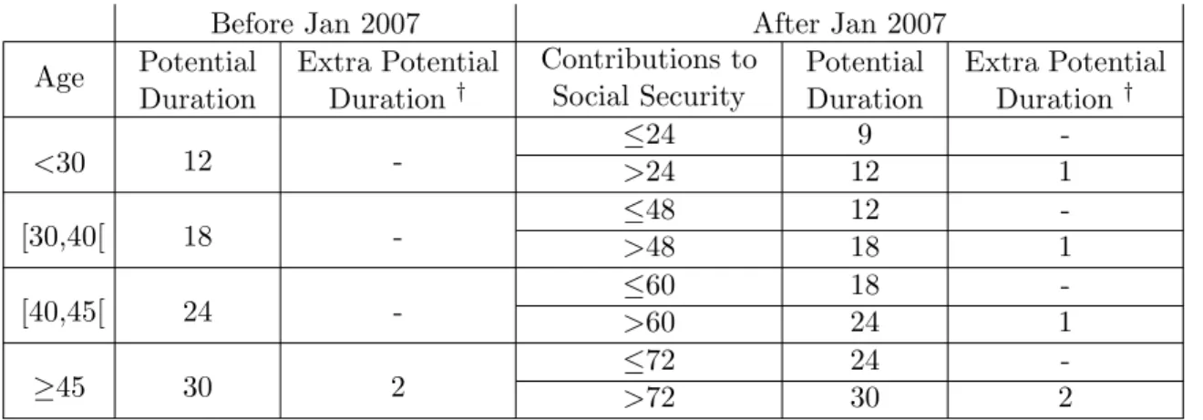
Finally the most noticeable change was that of potential duration of unemployment benefits. As it is summarized in table 1, the potential duration rule has decreased for the
8
Even though the reform was published in November of 2006, most of the changes have only taken place since January of 2007.
9
unemployed with small career histories. Conversely, the individuals aged below 45 years old with longer career histories have benefited from one, two, three, or four extra months of potential duration of unemployment, according to the length of the past job history. Even though the applied changes covered a large share of the unemployed individuals, it was still possible to observe individuals with the same potential duration of unemployment benefit as before.
Table 1: Potential Duration Rules (all values in months except age)
Before Jan 2007 After Jan 2007
Age Potential Duration Extra Potential Duration † Contributions to Social Security Potential Duration Extra Potential Duration † <30 12 -≤24 9 ->24 12 1 [30,40[ 18 -≤48 12 ->48 18 1 [40,45[ 24 - ≤60>60 1824 1 -≥45 30 2 ≤72 24 ->72 30 2 †
for each 5 years of contributions in the 20 years previous to the date of unemployment
The data used in this study covers both rules as the period in analysis goes from January 2005 until March 2012.
3
Data
3.1 Data source
The database in use is a sample from the panel of Microdados do Sistema de Informa¸c˜ao da Seguran¸ca Social, with monthly data on the unemployment beneficiaries inflow between January 2005 and March 2012, in Portugal. This sample contains 39 972 unemployment bene-ficiaries with an extensive amount of information. It includes basic individual information, job history, and all the necessary details about the unemployment benefits. At an individual level there is information on gender, birth and death dates, and birth and living places. In terms of job history, the database comprises information since 1941. Even though monthly earnings
(split into base wage, and regular and non-regular benefits) are only available between 2005 and 2012, the database includes the type of job (self-employed or not), basic details on the company (region and economic activity sector) and the starting and ending date of each job since the very first job of the oldest individual in the sample. The unemployment informa-tion comprises the start and ending dates (or potential ending date, in case of censoring) of the spells, the benefit amount, the type of benefit and the participation on any type of training or occupational program. Finally, there is also information other types of exit beside re-employment, such as illness, disability, maternity, social income or old-age pension.
3.2 Sample Construction
Due to the complexity of the database we have filtered the sample in order to enable the comparison of our results with previous studies in the literature. Therefore, among the 39 972 unemployed, we have decided to focus the analysis on the individuals that were covered by the basic unemployment benefit, i.e., by the unemployment insurance system described in section 2. After that, we have excluded from the analysis all the individuals that have manipulated extensions in the potential duration of unemployment benefits.10 Such decision resulted in the
exclusion of 19% of the 29 760 individuals selected in the first step. Additionally, we have also excluded the individuals that have anticipated their pension because of the change in the rule that also occurred since January 2007. Finally, we have also excluded all the individuals for which there was lack of information on any of the explanatory variables used in the regressions. Such options lead us to a sample constituted by 18 543 individuals. Descriptive statistics are presented in appendix A.
10Manipulated extensions of the basic unemployment benefit include training, extra benefits such as
parent-hood, disease, or disability benefits during the period of unemployment insurance. Unemployment beneficiaries are enabled delay their potential duration of the unemployment benefit in case they start receiving a disability, disease or parenthood benefit. In the case of training support the potential duration is adjusted in the end of the period. Moreover, training is not equally accessible to all the beneficiaries. Finally, in case of low income benefits there is no implication on the potential duration. Given this, we have not dropped beneficiaries that accumulated unemployment benefits with low income support.
4
Empirical Model
In order to evaluate the impact of the unemployment duration on the post-unemployment wage we need to identify the value of α1 in the following wage equation (in log form):
log(P ostWi) = α0+ α1log(U Di) + X0β + ui (1)
where P ostWi is the post-unemployment wage of individual i, U Di is the duration of the
spell of unemployment prior to re-employment, and X includes other covariates such as pre-unemployment wage, gender and age.
However, if equation 1 is estimated by Ordinary Least Squares (OLS) it is very likely that the value of α1 is biased. Without information on the reservation wage (which is the
case in administrative data), one cannot identify whether the post-unemployment wage is being determined by the unemployment duration (through stigma, loss of job-specific human capital, and other channels discussed in section 1), or whether the post-unemployment wage is actually determining the unemployment duration. According to job search theory, the un-employed individual sets a reservation wage such that all the wage offers below that threshold are rejected (or analogously, all the wage offers greater than the threshold are accepted). 11
Therefore, the correlation between post-unemployment wage and reservation wage tends to be high. Given this, if the unemployed sets a high reservation wage, it is likely that she will not get such a high wage offer in the beginning of the spell. Consequently, as the unem-ployed individual approaches the end of the potential duration of unemployment benefits, the reservation wage must start falling until she finds a job offer for which the wage is above the predetermined threshold. In result, the length of the unemployment spell ends up being deter-mined by the reservation wage, which is then highly correlated with the post-unemployment wage.
In order to get around this simultaneity bias issue, we employ a control function
ap-11
proach.12 In a first stage, we employ a survival model to predict the joblessness duration.13 Since this step is not estimated in a linear fashion, one cannot directly plug in the predicted duration as a regressor in the re-employment wage equation. Accordingly, instead of plugging the predicted variable in the second stage, we plug the residual of the first stage. By keeping in the wage equation exactly same the regressors as before (including the potential endoge-nous variable), the residual from the first stage (ν) will correct any potential endogeneity, thus cleaning out the effect of unemployment duration on re-employment wage.14 Under this method, equation (1) becomes:
log(P ostWi) = φ0+ φ1log(U Di) + φ2νi+ X0β + ui (2)
Thus, the control function approach enables us to both to estimate a unbiased causal effect of unemployment duration on post-unemployment wages (φ1) as well as to test the
endogeneity present in equation (1) – through the analysis of the statistical significance of (φ2). For robustness purposes the following equation is also estimated:
log(P ostWi) − log(P reWi) = γ0+ γ1log(U Di) + γ2νi+ X0β + ui (3)
Using this last specification, where the dependent variable is the difference between post- and pre-unemployment wages, we can discount any individual unobserved permanent heterogeneity (Bartel and Borjas, 1981).
12
For control function approach see Wooldridge, 2015
13In section 5 we present the argument for the use of a survival model in the first stage. In the same section,
three subsections briefly present and justify three alternative strategies employed in the estimation of this first step.
14Even after this correction, there is another concern related with the validity of the usual standard errors.
Since the two stages are estimated in separate steps, we have bootstrapped our sample in 1000 repetitions for all the equations.
5
Identification Strategies for the Unemployment Duration
As it is widely proven in the literature, a change in the potential duration of unem-ployment benefits usually impacts the actual joblessness duration in the same direction.15 Therefore, recurring to the 2007 reform on the potential length of unemployment benefits we obtain an exogenous variation in unemployment duration which is then used to predict the average joblessness duration.16
When estimating the first stage of this method, one should have in mind that a consid-erable fraction of our sample reveals incomplete spells of unemployment duration. Thus, the fact that OLS estimates do not take into account the right-censoring in duration may lead to biased results. One alternative could be to run the first stage regression only for the com-pleted spells. However, this would still be far away from predicting the actual unemployment duration distribution. To take into account the right-censoring in unemployment duration we estimate the first stage using an accelerated failure time model (Kalbfleisch and Pretice 1980) with a lognormal distribution.17 Moreover, by using a survival analysis model, we also take advantage on the information of the incomplete spells as a potential correction of any selectivity into re-employment.
In the next subsections we present three alternative instruments to predict joblessness duration: the potential duration of unemployment benefit, the change in the potential dura-tion of unemployment benefit due to the reform in January 2007, and the age discontinuity in the potential duration of unemployment benefit.
5.1 Strategy 1: Potential Duration of Unemployment Benefit
For a benchmark we use the potential duration of unemployment benefit. As mentioned in Section 4, the literature usually reports a strong (positive) relation between this variable and the joblessness duration. Moreover, the fact that during the period in analysis there is
15
See Narendranathan et al. (1985), Meyer (1990), Katz and Meyer (1990), Van Ours and Vodopivec (2006), Addison and Portugal (2004, 2008) and Lopes (2015)
16
See section 2 for a detailed description on the institutional change
17Another alternative could be to use the proportional hazards model but note that those models are subject
to the choice of the conditional probability distribution. Moreover, the accelerated failure time models tend to perform better in case of omitted covariates.
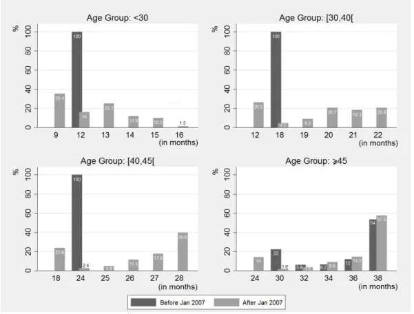
a change in rules of potential duration favours the identification of the joblessness durations in our sample. In order to give the reader a visual perspective of the actual change in the distribution of the potential duration of unemployment benefits in out sample, we present the following figures with calculations from our sample:
Figure 1: Percentage of individuals by age group and potential duration of unemploy-ment benefit, before and after the 2007 reform
Through the analysis of these four figures, we achieve three main conclusions. Firstly, the fact that potential durations of unemployment benefits for individuals aged below 45 years old were no longer defined solely by the age, after the reform. Secondly, the number of individuals that was entitled to the minimum potential duration within age group decreased along age. Conversely, the number of individuals that was entitled to the maximum potential duration within each age group increased along age. Thirdly, the major change within the last age group was a shift from 30 to 24 months of potential duration because the potential duration for this group was already conditioning on working experience, before the reform.
5.2 Strategy 2: Change in Potential Duration of Unemployment Benefit
Alternatively to the first strategy, we use the change in the potential duration of un-employment benefit. This variable is defined as the change, in months, between the potential duration of unemployment benefit for each individual and the rules in place before January 2007. Therefore, all the individuals that entered in the system before that date will have a value of zero in this variable. For all the unemployed that entered into the system after the reform, the change may either assume positive, negative or zero value. For the latter individuals we observe the following distribution in our sample:
Table 2: Change, in months, between 2007 and 1999 potential duration of unemployment benefit rules, for individuals unemployed after January 2007
Change Individuals Percentage
-6 1959 13.95 -3 1259 8.97 0 5042 35.90 +1 1354 9.64 +2 1475 10.50 +3 1452 10.34 +4 1503 10.70
From the table above we observe that only approximately 36% of the individuals which became unemployed after January 2007, were entitled to the same rules as if they entered into unemployment during the previous system. Additionally, about 23% were entitled to shorter potential durations, that is, 23% of the beneficiaries have not reached the minimum period of contributions necessary, in order to be entitled to at least the same potential duration as before. Finally, roughly 41% has actually benefited from the institutional change applied due to their longer job histories.
The main goal of this alternative strategy is to use a variable that is not as correlated with age and previous Social Security contributions as the potential duration itself. For example, using the potential duration we already know that an individual eligible to 13 months must have less than 30 years old. Using the change in rules, that individual is attributed with the value +1. With the new definition, this individual may either be entitled to 13, 19 or 25 months of potential duration, which covers a range of age up until 45 years old.
Another example is, if an individual was entitled to less six months than in previous rules, that may either mean that the individual’s age lies between 30 and 40 years old and the past contributions are not larger than 48 months, or that the individual’s age lies between 40 and 45 years old and the past contributions are not larger than 60 months, or even that the individual’s age is larger than 45 years old and the past contributions are not larger than 72 months. Summarily, the correlations are the following:
Table 3: Correlation between strategies 1 and 2 and other determinants of unemployment duration
Potential ∆ Potential
Age 0.8996 -0.0274
Experience 0.5183 0.1793
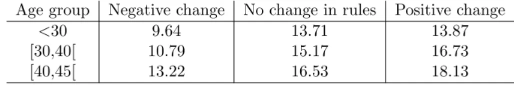
On top of this advantage, we argue that this is a good strategy because the individuals that have benefited from the new rules have actually had longer spells of unemployment in comparison with those that were entitled to the same rules as before January 2007:
Table 4: Average actual duration of unemployment benefits, by age group and difference between 2007 and 1999 potential duration of unemployment benefit rules
Age group Negative change No change in rules Positive change
<30 9.64 13.71 13.87
[30,40[ 10.79 15.17 16.73
[40,45[ 13.22 16.53 18.13
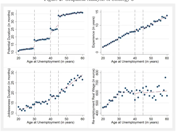
5.3 Strategy 3: Age Discontinuity in Potential Duration of Unemployment Benefit
Finally, following Addison and Portugal (2008), we look at the discontinuity in potential duration of unemployment benefits generated by the age groups in order to get rid of the correlation between the the potential duration of unemployment benefits and experience. This last strategy relies on a dummy variable that assumes the value 1 if the individual has 30, 40 or 45 years old and 0 if the individual has 29, 39 or 44 years old at the date of unemployment. Assuming that experience is constant within a range of two years of age, this variable captures
the difference in potential duration generated by the change in age groups.18
For the individuals unemployed before January 2007, with 29, 39 or 44 years old, one more year of age means six additional months of potential duration. For the individuals unemployed after January 2007, one more year of age may actually lead to no change in the potential duration of the unemployment benefit. That happens when we look at a 29 years old unemployed with experience between 24 and 48 months; or at a 39 years old unemployed with experience between 48 and 60 months; or at a 44 years old unemployed with experience between 60 and 72 months. In those three cases, one more year of age leads to no change in the potential duration of unemployment benefit. In all other cases, the individual may be entitled up to additional 10 months of potential duration, if unemployed after January 2007. In the table of graphs below, we provide evidence towards the validity and strength of this last strategy:
Figure 2: Graphical Analysis of Strategy 3
From the four graphs above we observe that there are clear discontinuities in the
poten-18
tial duration which are reflected, at a lower strength, in the joblessness duration. Moreover, once the same pattern does not apply to experience (control variable) and re-employment wage (outcome variable in the second stage) there is, at least, no clear relationship between age at unemployment and these two variables, which favours the validity of this strategy.
6
Results
In the next subsection we present the OLS estimates for the wage and wage loss/gain equation, and briefly discuss their coefficients. In the following subsection we present the results on each of the three empirical strategies described in section 5. First stages of the control function approach are provided in appendix B.
6.1 OLS results
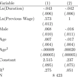
Table 5 provides the OLS estimates for the equations wage and wage loss/gain equations. The coefficient estimate associated to unemployment duration is negative and significant for both specifications. That means, an increase of 10% in the joblessness duration is estimated to decrease the post unemployment wage in 0.4%, on average, ceteris paribus. Such result does not change when we look at the impact on the wage change. Both effects go in line with the theories reviewed in section 1. Hence, along the spell of unemployment, the individual decreases the reservation wage until it falls below the previous wage.
As for the other coefficients we observe a positive large elasticity with respect to the previous wage, a significant gender gap towards male individuals and positive but decreasing effect from age. Note that in column (1) the previous wage was also capturing part of the gender and age wage differentials. Therefore, once we look at wage loss, in column (2), the opposite sign in those coefficients should be expected. For example, since being a male individual contributes to a higher re-employment wage, then male individuals should expect smaller wage losses after the spell of unemployment.
As it was already mentioned, theory suggests that re-employment wage and duration may be simultaneously defined. A few studies have addressed this issue by estimating the
Table 5: Re-employment wage equations Variable (1) (2) Ln(Duration) -.043 -.042 (.006) (.006) Ln(Previous Wage) .573 1 (.012) Male .068 -.016 (.010) (.011) Age .007 -.017 (.004) (.004) Age2 -.00009 .00020 (.00005) (.00005) Constant 2.515 .237 (.095) (.075) R2 .275 .051 N 8 423
Notes: usual standard errors in parenthesis below the estimates. The equations also include seven year dummies and three quarter dummies, according to the date of re-employment, and economic activity sector dummies.
structural parameters of both wage and duration equations.19 In the next section, we consider a control function approach to correct for the possible presence of endogeneity in unemploy-ment duration.
6.2 Control Function Results
The results for each of the three strategies employed in the first stage are presented in appendix B. In the first strategy, results show evidence for the concern discussed in section 5.1. Since the potential duration is highly correlated with age, the coefficients on age groups yield a non-expected (negative) sign. However, that is compensated by the large and significant coefficient on potential duration. Consequently, when we use the change in potential duration rules, age reveals the expected (positive) sign. Finally, in the third strategy we confirm that longer duration spells are expected for the unemployed at the boundary of age groups.
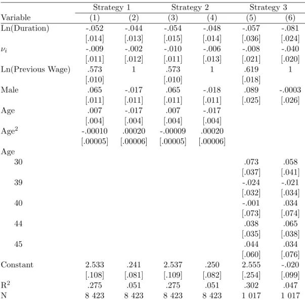
From table 6, we can depict two relevant conclusions. Firstly, the elasticity of
unem-19
Table 6: Re-employment wage equations using three different strategies to predict unemployment duration
Strategy 1 Strategy 2 Strategy 3
Variable (1) (2) (3) (4) (5) (6) Ln(Duration) -.052 -.044 -.054 -.048 -.057 -.081 [.014] [.013] [.015] [.014] [.036] [.024] νi -.009 -.002 -.010 -.006 -.008 -.040 [.011] [.012] [.011] [.013] [.021] [.020] Ln(Previous Wage) .573 1 .573 1 .619 1 [.010] [.010] [.018] Male .065 -.017 .065 -.018 .089 -.0003 [.011] [.011] [.011] [.011] [.025] [.026] Age .007 -.017 .007 -.017 [.004] [.004] [.004] [.004] Age2 -.00010 .00020 -.00009 .00020 [.00005] [.00006] [.00005] [.00006] Age 30 .073 .058 [.037] [.041] 39 -.024 -.021 [.032] [.034] 40 -.001 .034 [.073] [.074] 44 .038 .065 [.035] [.038] 45 .044 .034 [.060] [.076] Constant 2.533 .241 2.537 .250 2.555 -.020 [.108] [.081] [.109] [.082] [.254] [.099] R2 .275 .051 .275 .051 .302 .047 N 8 423 8 423 8 423 8 423 1 017 1 017
Notes: bootstrapped standard errors in parenthesis below the estimates. The equations also in-clude seven year dummies, three quarter dummies, according to the date of re-employment, and economic activity sector dummies.
ployment duration is consistently negative and significant along the three strategies. If the unemployment duration increases by 10%, the re-employment wage is expected to decrease be-tween 0.5% and 0.6%.20 A similar interpretation applies to the wage loss equations. Secondly, the coefficient associated to the control function approach is not statistically significant along the six specifications, thus pointing to the absence of endogeneity related to unemployment
20
Using the mean of joblessness duration in our sample, this means that each additional month implies an average decrease between 0.4% and 0.5% in re-employment wages.
duration. The remaining coefficients do not register relevant change in comparison with the OLS estimates. Note that, according to the strategy employed in the first strategy, we have chosen a different specification to capture the age effect. Since we only use the individuals with ages before and at the thresholds, the use of dummies (age 29 is the base group) seemed to be more appropriate than a concave specification.
7
Sensitivity Analysis
For purposes of robustness we assess or results in terms of sensitiveness along three dimensions: observables, estimation method, and the definition of re-employment wages. In terms of sensitiveness to observables, we check whether the effect of joblessness duration on re-employment wage varies along the period of analysis, across different pre-unre-employment wage quartiles, across different reasons of unemployment, and according to whether the individual has been re-employed in a different economic activity sector. Then, we test if our estimates are subject to change when estimated by two-stage least squares (2SLS, henceforth), as an alternative to the control function approach. For simplicity, we have chosen strategy 2 for all the robustness tests, namely with the logarithm of re-employment wage as dependent variable.21 Finally, in order to evaluate the persistence of the results obtained in the previous
section, we have analysed the impact of joblessness duration in re-employment wage earned one, three, and five years after the date of re-employment. All the results are reported in tables in appendix C.
7.1 Economic Crisis Period
The causal effect of unemployment duration on re-employment wages has been widely studied in the literature. Such a concern is most common in times of crisis, when
unemploy-21
The other specifications were also estimated and reflected no major changes in comparison to the results of the preferred specification. However, the non-significance of the third identification strategy was an exception when estimated by 2SLS, which probably is due to the nature of the discontinuity in this variable, as well as to the small number of observations in use in this strategy.
ment rises abruptly, and the the last crisis of 2007-2009 was not an exception.22
A major concern in our main estimates from table 6 could be the fact that there is a large period under our analysis in which Portugal was under a crisis environment. Such macroeconomic conditions have actually generated a catastrophic job destruction (Carneiro et al., 2014). In order to test whether the wage losses are explained by the increase in collective dismissals after 2009, we have run the same specification for individuals dismissed during the periods 2005-2008 and 2006-2007. In the first sample we have excluded the period of crisis between 2009 and 2012. In the second sample we have restricted the time frame even more in order to ensure that the effect of joblessness duration on re-employment wage is being identified by the variable referred in strategy 2, which uses the difference in unemployment benefits’ rules pre- and post-2007 reform. The estimates presented in the first column of table C1 show that the results in table 6 are not negatively biased (in magnitude) by the crisis environment in Portugal after 2009. Actually, the effect of joblessness duration increases when we restrict the period to the years immediately before and after the unemployment benefits’ reform, thus reinforcing the strength of strategy 2.
7.2 Distribution of Pre-unemployment Wages
A comparison of the estimates presented in table C2 shows that the impact of joblessness duration on the re-employment wage gets wider along the pre-unemployment wage distribu-tion, such that unemployed individuals with larger pre-unemployment wages get larger wages losses in re-employment. This result seems to be consistent with two characteristics of the labour market in Portugal. While the existence of a minimum wage goes in line with the positive (non-significant) impact observed in the first quantile, the evidence for backloaded compensation in Portugal (Blanchard, 2007 and Portugal, 2006) supports the fact that work-ers with higher pre-unemployment wages face larger wage losses after being unemployed.23 A similar result was find in Burda and Mertens (2001) for Germany.24
22According to Couch and Placzek (2010) and Couch, Jolly and Placzek (2011), earnings losses of displaced
workers are larger during recessionary times.
23See Saphiro and Stiglitz (1984) for a theoretical explanation 24
Centeno and Novo (2014) also found that low-wage workers tend to react less to benefit extensions, which may also explain the non-significant impact we observe in the first quantile of the pre-unemployment wage
7.3 Reasons of Unemployment
In terms of reasons of unemployment we find that only two of them reveal a statistically significant change on the impact of unemployment duration on the re-employment wage.25 In the first column of table C3 we observe that, on average, re-employment wages are higher for those which were displaced due to firm closure or extinguished job position. This positive difference may be related to the fact that those unemployment reasons are not related with the quality of the unemployed, and therefore it must not be, on average, more difficult for them to get a relatively better paid job, in comparison to individuals that were displaced for other reasons. Apart from the average difference, there seems to be no change in terms of the impact of unemployment duration on re-employment wages for those which were displaced due to firm closure or extinguished job position. On the other hand, when we look at the unemployed that were fired under a mutual agreement, in the second column of table C3, we observe the opposite results. This type of unemployed get, on average, the same wage as the other unemployed but each additional month of unemployment leads to a even larger negative effect on re-employment wages. Under such results, there seems to be evidence for moral hazard behaviour during the spell of unemployment according to the reason of displacement.
7.4 Job Change Between Economic Sectors
Table C4 reports the impact of joblessness duration on the re-employment wage for individuals that have moved, or not, economic activity sector between the pre- and post-unemployment jobs, respectively. The estimates point towards smaller losses for the individu-als that moved for another industry. This result could be explained by the matching literature referred in section 1. However, such effect revealed to be non-significant.
distribution.
25The reasons of unemployment subject to this test were the following: collective dismissal, employer decision,
7.5 Alternative Methodology
Additionally to the sensitiveness with the observables we have also considered an alter-native methodology. Instead of recurring to the control function method, we have employed the traditional 2SLS, after removing the crisis period in order to minimize the censoring in joblessness durations which could bias the estimates in the first stage. The results presented in the third column of table C5 are similar to that of the third column in table 6.
7.6 Impact on Future Wages
Finally, we have also estimated the same specification for different wages along the first 5 years in re-employment. In table C6 we observe that the effect of unemployment duration on the re-employment wage after one year of work in the new job does not seem to change relative to the effect on the first re-employment wage. Actually, when we look at the wage growth (in the first year) in the new job we observe no statistical significant effect from the duration in the preceding unemployment spell. Such results are also observed when we look at wages that are three years of distance from the date of re-employment but the statistical significance vanishes when we do the same analysis with wages five years after re-employment. This pattern points towards relative persistent effects of unemployment duration on re-employment wages. One of the possible explanations could be the relatively short tenure in re-employment. In case the recently re-employed fall into unemployment again or transit to another job, any returns to recent tenure are lost. In fact, we observe that roughly 45% of the re-employed face a new unemployment spell in the first six years of re-employment. Moreover, after one year of re-employment only 37% of the workers remain in the same company that hired them after unemployment. However, when we look at the impact of unemployment duration on re-employment tenure, there seems to be no impact. Such a result was also found by Nekoei and Weber (2015).
8
Conclusions
A broad range of methodologies have been applied to estimate the causal effect of un-employment duration on re-un-employment wages. Without information on the reservation wage (which is the case in administrative data), one cannot identify whether the post-unemployment wage is being determined by the unemployment duration (through stigma, loss of job-specific human capital, and other channels discussed in section 1), or whether the post-unemployment wage is actually determining the unemployment duration. Our study adds two main contri-butions to this literature.
Taking advantage of an institutional reform on the potential duration of unemploy-ment benefits, in January of 2007, in Portugal, we employ three different strategies to predict the unemployment duration. In a first specification, we use the potential duration of unem-ployment benefit itself. While this variable yields a strong positive effect on the joblessness duration, it is strongly correlated with age and experience. Therefore, in order to clean out both effects, we present two alternative specifications. One is defined as the difference in the rules of potential duration of unemployment benefits, generated by the reform. Whereas this kind of policies usually rely on a general increase (or a general decrease) of the potential duration of the beneficiaries, this policy contains a unique feature. While 41% have benefited from longer potential duration of unemployment benefits, 23% of the individuals that became unemployed after January 2007 were entitled to smaller potential duration of unemployment benefits. Using this strategy, we can get rid of the correlation with age and even decrease substantially the correlation with experience. Finally, using the age discontinuity in potential duration of unemployment benefits, we capture the causal effect of longer potential durations, while age and experience are roughly constant.
The second main contribution is related to the procedure employed in the control func-tion approach. Firstly, by considering the informafunc-tion on the incomplete spells of unemploy-ment, we get more accurate estimates on the predicted duration (Addison and Portugal, 1989). Moreover, it can be interpreted as an attempt to solve any selectivity on re-employment. Sec-ondly, since we have estimated the first stage with a non-linear model (accelerated failure
time model), we have not directly plugged the predicted duration in the wage equation but the residual of the first stage equation, instead. Our estimates reveal that each additional month of unemployment duration leads to statistically significant decrease of approximately 0.5% in re-employment wages.26 The estimate goes in line with Addison and Portugal (1989) and Schmieder et al. (2015), even though at a smaller scale. Such difference may lie behind the fact that responsiveness of real wages to unemployment changes may have declined over the last decade (Marques et al., 2010).
The contributions of our results do not restrict to the estimate of the causal effect of unemployment duration on re-employment wages. Actually, they lead to important policy implications. As pointed in Nekoei and Weber (2015), a positive effect would suggest that unemployment insurance subsidize search and not just leisure, which is not the case when we look at our sample. When we analyse the sensitiveness of our results, there seems to be presence of a moral hazard behaviour according to the reason of unemployment. Moreover, the negative effect of unemployment duration on re-employment wages shows a relatively high persistence, which only vanishes three years after the date of re-employment. Therefore, additional job assistance programs may be justified in Portugal (Carneiro et al., 2015).
Reconciling our results with the decrease on potential duration of unemployment ben-efits in Portugal in 2012, from a top 38 months to 26 months, we expect that, if the actual joblessness duration changes in the same direction, the unemployed can actually benefit from wage gains after displacement. Nevertheless, the fact that the social subsequent unemploy-ment benefit has increased with the reform of 2012 for individuals aged above 40 years old may lead to a counteracting effect in re-employment wages. A wider and more recent set of the data is then of the utmost importance in order to evaluate the effect of recent policies.
26
Even though the effect is somewhat larger than the OLS estimates, the control function correction points to the absence of endogeneity in the duration of unemployment on the wage equation.
References
[1] Addison, J. T., and Blackburn, M. L. (2000). “The effects of unemployment insurance on post-unemployment earnings”. Labour Economics, Vol. 7(1), pp. 21-53
[2] Addison, J. and Portugal, P. (1989). “Job displacement, relative wage changes, and duration of unemployment”, Journal of Labor Economics, pp. 281-302.
[3] Addison, J. T., and Portugal, P. (2004). “How does the unemployment insurance system shape the time profile of jobless duration?”. Economics Letters, Vol. 85(2), pp. 229-234. [4] Addison, J. T., and Portugal, P. (2008). “How do different entitlements to unemploy-ment benefits affect the transitions from unemployunemploy-ment into employunemploy-ment?”. Economics Letters, Vol. 101(3), pp. 206-209.
[5] Arulampalam, W. (2001). “Is unemployment really scarring? Effects of unemployment experiences on wages”. Economic Journal, pp. 585-606.
[6] Bartel, A. P., and Borjas, G. J. (1981). “Wage growth and job turnover: an empirical analysis”. In Studies in Labor Markets (pp. 65-90). University of Chicago Press. [7] Becker, G. S. (1962). “Investment in human capital: A theoretical analysis”, The journal
of political economy, pp. 9-49.
[8] Blanchard, O. (2007). “Adjustment within the euro. The difficult case of Portugal”. Portuguese Economic Journal, Vol. 6(1), pp. 1-21.
[9] Burda, M. C., and Mertens, A. (2001). “Estimating wage losses of displaced workers in Germany”. Labour Economics, Vol. 8(1), pp. 15-41.
[10] Cahuc, P. and Zylberberg, A. (2004). “Labor economics”, MIT press.
[11] Card, D., Chetty, R., and Weber, A. (2006). “Cash-on-hand and competing models of intertemporal behavior: New evidence from the labor market” (No. w12639). National Bureau of Economic Research.
[12] Carneiro, A., Portugal, P., and Varej˜ao, J. (2014). “Catastrophic job destruction during the Portuguese economic crisis”. Journal of Macroeconomics, Vol. 39, pp. 444-457. [13] Carneiro, A., Portugal, P., and Raposo, P. (2015) “Decomposing the Wage Losses of
Dis-placed Workers: The Role of the Reallocation of Workers into Firms and Job Titles”. IZA Discussion Paper No9220
[14] Centeno, M. and Novo, ´A. A. (2006). “The impact of unemployment insurance on the job match quality:a quantile regression approach”, Empirical Economics, Vol. 31, pp. 905-919.
[15] Centeno, M., and Novo, ´A. A. (2014). “Do Low - Wage Workers React Less to Longer Un-employment Benefits? Quasi - Experimental Evidence”. Oxford Bulletin of Economics and Statistics, Vol. 76(2), pp. 185-207.
[16] Carrington, W. J., and Fallick, B. C. (2015). “Do We Know Why Earnings Fall with Job Displacement?”.
[17] Chesher, A. and Lancaster, A. (1984). “Simultaneous Equations with Endogenous Haz-ards”. Studies in Contemporary Economics, Vol. 11, pp. 16-44
[18] Couch, K. A., and Placzek, D. W. (2010). “Earnings losses of displaced workers revisited”, The American Economic Review, pp. 572-589.
[19] Couch, K. A., Jolly, N. A., and Placzek, D. W. (2011). “Earnings losses of displaced workers and the business cycle: an analysis with administrative data”. Economics Letters, Vol. 111(1), pp. 16-19.
[20] Gibbons, R., and Katz, L. (1989). “Layoffs and lemons”. National Bureau of Economic Research (No. w2968)
[21] Hildreth, A. K., and Oswald, A. J. (1997). “Rent-sharing and wages: evidence from company and establishment panels”. Journal of Labor Economics, pp. 318-337.
[22] Jovanovic, B. (1979). “Job matching and the theory of turnover”. The Journal of Political Economy, pp. 972-990.
[23] Kalbfleisch, J. D., and Prentice, R. L. (2011). “The statistical analysis of failure time data” Vol. 360. John Wiley & Sons.
[24] Katz, L. F., and Meyer, B. D. (1990). “The impact of the potential duration of unem-ployment benefits on the duration of unemunem-ployment”. Journal of public economics, Vol. 41(1), pp. 45-72.
[25] Kessler, R. C., House, J. S., and Turner, J. B. (1987). “Unemployment and health in a community sample”. Journal of health and social behavior, pp. 51-59.
[26] Lalive, R. (2007). “Unemployment benefits, unemployment duration, and post-unemployment jobs: A regression discontinuity approach”. The American economic review, pp. 108-112.
[27] Lazear, E. P. (1981). “Agency, earnings profiles, productivity, and hours restrictions”. The American Economic Review, pp. 606-620.
[28] Lopes, M. C. (2015). “The impact of unemployment insurance potential duration on the joblessness duration”. Mimeo
[29] Lundberg, S. (1985). “The added worker effect”. Journal of Labor Economics, pp. 11-37. [30] Marques, C., Martins, F. and Portugal, P. (2010). “Price and wage formation in
Portu-gal”. Working Paper Series 1225, European Central Bank.
[31] Meyer, B. (1990). “Unemployment Insurance and Unemployment Spells”. Econometrica. Vol. 58(4), pp. 757-782
[32] Narendranathan, W., Nickell, S., and Stern, J. (1985). “Unemployment benefits revis-ited”. The Economic Journal, pp. 307-329.
[33] Nekoei, A., and Weber, A. (2013). “Does Extending Unemployment Benefits Improve Job Quality?”. Mimeo, Harvard University, Cambridge, MA.
[34] Portugal, P. (2006). “Wage setting in the Portuguese labor market: a microeconomic approach”. Economic Bulletin, Vol. 78, pp. 89-100.
[35] Shapiro, C., and Stiglitz, J. E. (1984). “Equilibrium unemployment as a worker discipline device”. The American Economic Review, pp. 433-444.
[36] Schmieder, J. F., von Wachter, T., and Bender, S. (2012). “The Effects of Extended Unemployment Insurance Over the Business Cycle: Evidence from Regression Discon-tinuity Estimates Over 20 Years”. The Quarterly Journal of Economics, Vol.. 127(2), pp. 701-752.
[37] Schmieder, J. F., von Wachter, T., and Bender, S. (2015). “The Causal Effect of Unem-ployment Duration on Wages: Evidence from UnemUnem-ployment Insurance Extensions”. American Economic Review, forthcoming.
[38] Van Ours, J. C., and Vodopivec, M. (2006). “How shortening the potential duration of unemployment benefits affects the duration of unemployment: Evidence from a natural experiment”. Journal of Labor Economics, Vol. 24(2), pp. 351-378.
[39] Van Ours, J. C., and Vodopivec, M. (2008). “Does reducing unemployment insurance generosity reduce job match quality?”. Journal of Public Economics, Vol. 92(3), pp. 684-695.
[40] Wooldridge, J. M. (2015), “Control Function Methods in Applied Econometrics”, Journal of Human Resources, Vol 50(2), pp. 420-445.
Appendices
Appendix A
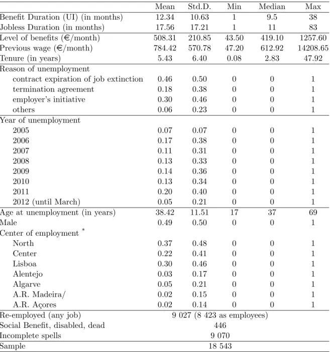
Table A 1: Descriptive statistics - Full Sample
Mean Std.D. Min Median Max
Benefit Duration (UI) (in months) 12.34 10.63 1 9.5 38
Jobless Duration (in months) 17.56 17.21 1 11 83
Level of benefits (e/month) 508.31 210.85 43.50 419.10 1257.60 Previous wage (e/month) 784.42 570.78 47.20 612.92 14208.65
Tenure (in years) 5.43 6.40 0.08 2.83 47.92
Reason of unemployment
contract expiration of job extinction 0.46 0.50 0 0 1
termination agreement 0.18 0.38 0 0 1 employer’s initiative 0.30 0.46 0 0 1 others 0.06 0.23 0 0 1 Year of unemployment 2005 0.07 0.07 0 0 1 2006 0.17 0.38 0 0 1 2007 0.11 0.31 0 0 1 2008 0.13 0.33 0 0 1 2009 0.14 0.36 0 0 1 2010 0.13 0.34 0 0 1 2011 0.20 0.40 0 0 1 2012 (until March) 0.05 0.21 0 0 1
Age at unemployment (in years) 38.42 11.51 17 37 69
Male 0.49 0.50 0 0 1 Center of employment* North 0.37 0.48 0 0 1 Center 0.22 0.41 0 0 1 Lisboa 0.30 0.46 0 0 1 Alentejo 0.03 0.17 0 0 1 Algarve 0.05 0.21 0 0 1 A.R. Madeira/ 0.02 0.15 0 0 1 A.R. A¸cores 0.02 0.14 0 0 1
Re-employed (any job) 9 027 (8 423 as employees)
Social Benefit, disabled, dead 446
Incomplete spells 9 070
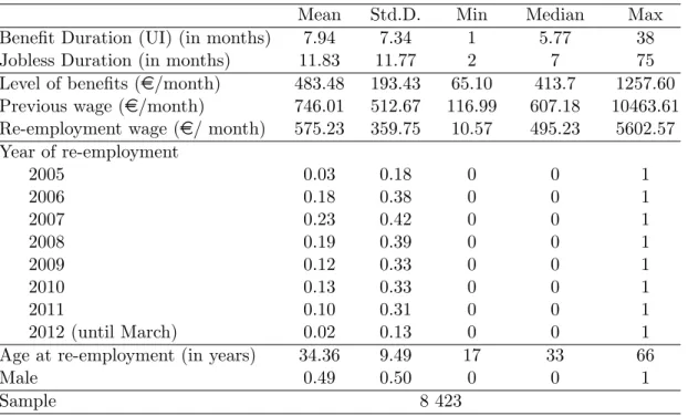
Table A 2: Descriptive Statistics - Re-employed Sample
Mean Std.D. Min Median Max
Benefit Duration (UI) (in months) 7.94 7.34 1 5.77 38
Jobless Duration (in months) 11.83 11.77 2 7 75
Level of benefits (e/month) 483.48 193.43 65.10 413.7 1257.60 Previous wage (e/month) 746.01 512.67 116.99 607.18 10463.61 Re-employment wage (e/ month) 575.23 359.75 10.57 495.23 5602.57 Year of re-employment 2005 0.03 0.18 0 0 1 2006 0.18 0.38 0 0 1 2007 0.23 0.42 0 0 1 2008 0.19 0.39 0 0 1 2009 0.12 0.33 0 0 1 2010 0.13 0.33 0 0 1 2011 0.10 0.31 0 0 1 2012 (until March) 0.02 0.13 0 0 1
Age at re-employment (in years) 34.36 9.49 17 33 66
Male 0.49 0.50 0 0 1
Appendix B
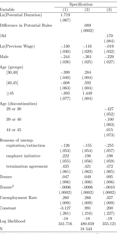
Table B 1: Accelerated Failure Time Unemployment Duration Equations
Specification
Variable (1) (2) (3)
Ln(Potential Duration) 1.719 (.067)
Difference in Potential Rules .089 (.0002) Old .170 (.084) Ln(Previous Wage) -.130 -.116 -.019 (.030) (.029) (.032) Male -.244 -.261 -.229 (.026) (.025) (.027) Age (groups) [30,40[ -.399 .284 (.040) (.004) [40,45[ -.608 .592 (.063) (.004) ≥45 -.393 1.449 (.077) (.004) Age (discontinuities) 29 or 30 -.427 (.052) 39 or 40 -.100 (.063) 44 or 45 .015 (.073) Reasons of unemp. expiration/extinction -.126 -.155 -.255 (.053) (.054) (.057) employer initiative .222 .198 .198 (.055) (.056) (.059) termination agreement .425 .421 .472 (.061) (.062) (.065) Tenure .047 .049 .095 (.006) (.006) (.006) Tenure2 -.0006 -.0006 -.0010 (.0002) (.0002) (.0002) Unemployment Rate .260 .266 .327 (.009) (.009) (.009) Constant -3.127 .991 .200 (.261) (.216) (.227) Log likelihood -18 341.716 -18 480.659 -19 355.121 N 18 543
Notes: standard errors in parenthesis below the estimates. The equations also include six region dummies.
Appendix C
Table C 1: Re-employment wage equations by year of unemployment 2005-2009 2006-2007 Variable (1) (2) Ln(Duration) -.048 -.064 [.012] [.018] νi -.009 .007 [.012] [.016] R2 .310 .311 N 6 478 3 992
Notes: bootstrapped standard errors in parenthesis be-low the estimates. The equation also includes pre-unemployment wage, male dummy, quadratic specifi-cation of age, seven year dummies, three quarter dum-mies, according to the date of re-employment, and economic activity sector dummies.
Table C 2: Re-employment wage equation
Effect of unemployment duration by pre-unemployment wage quartiles Second Stage
Variable (1)
Ln(Duration) -.005
[.014] Ln(Duration) ×1 (506e< Previous Wage ≤ 613 e) -.006 [.015] Ln(Duration) ×1 (613e< Previous Wage ≤ 841 e) -.051 [.014] Ln(Duration) ×1 (Previous Wage > 841 e) -.104 [.015]
νi -.001
[.012]
1 (506 e< Previous Wage ≤ 613 e) .081
[.031]
1 (613 e< Previous Wage ≤ 841 e) .268
[.028]
1 (Previous Wage > 841e) .749
[.033]
R2 .221
N 8 423
Table C 3: Re-employment wage equation
Effect of unemployment duration by reason of unemployment
Variable (1) (2)
Ln(Duration) -.056 -.064
[.014] [.013]
Ln(Duration) ×1 (Extinguished firm/job position) -.020 [.016]
Ln(Duration) ×1 (Mutual agreement) -.040
[.012]
νi .014 .011
[.012] [011]
1 (Extinguished firm/job position) .072
[.039]
1 (Mutual agreement) -.039
[.028]
R2 .276 .277
N 8 423 8 423
Notes: see notes of table C1.
Table C 4: Re-employment wage equation
Effect of unemployment duration by pre-unemployment economic activity sector movement Second Stage
Variable (1)
Ln(Duration) -.046
[.014] Ln(Duration) ×1 (New Job economic activity 6= Last Job economic activity) -.003 [.011]
νi .008
[.010] 1 (New Job economic activity 6= Last Job economic activity) -.035 [.023]
R2 .277
N 8 423
Table C 5: Re-employment wage equation estimated by 2SLS Second Stage Variable (1) Ln(Duration) -.059 [.022] Ln(Previous Wage) .573 [.017] Male .078 [.011] Age .003 [.004] Age2 -.00004 [.00005] Constant 2.577 [.114] R2 .310
First Stage F-test 185.14
N 6 478
Notes: see notes of table C1.
Table C 6: Re-employment wage equation
Effect of unemployment duration on re-employment wages after 1 year, 3 years and 5 years 1 year 1 year growth 3 years 3 years growth 5 years 5 years growth Variable (1) (2) (3) (4) (5) (6) Ln(Duration) -.058 .001 -.063 .007 .005 .063 [.012] [.013] [.016] [.018] [.034] [.040] νi .012 .012 .026 .015 -.026 -.034 [.011] [.012] [.016] [.018] [.031] [.035] R2 .331 .007 .349 .016 .331 .046 N 5 853 5 853 3 810 3 810 1 383 1 383
Nova School of Business and Economics Faculdade de Economia
Universidade Nova de Lisboa Campus de Campolide 1099-032 Lisboa PORTUGAL Tel.: +351 213 801 600
![Table C 1: Re-employment wage equations by year of unemployment 2005-2009 2006-2007 Variable (1) (2) Ln(Duration) -.048 -.064 [.012] [.018] ν i -.009 .007 [.012] [.016] R 2 .310 .311 N 6 478 3 992](https://thumb-eu.123doks.com/thumbv2/123dok_br/15883555.1089560/32.918.287.632.144.311/table-employment-wage-equations-year-unemployment-variable-duration.webp)
