MEMOIRE DE RECHERCHE
2013/2014
NOM et PRENOM de l’auteur: BRANDÃO, Sara
SUJET DU MEMOIRE
How is goodwill impairment driven by relative firm performance?
Evidence from Germany
NOM DU DIRECTEUR DE RECHERCHE: Professor Christopher HOSSFELD
CONFIDENTIEL
NonLa diffusion de ce recueil est strictement réservée à ESCP Europe.
How is goodwill impairment driven by firm performance?
Evidence from Germany
Sara Fontes Coutinho Mesquita Brandão
(Student e123377 at ESCP-Paris; 152112024 at UCP-CLSBE)
Research advisor: Professor Christopher Hossfeld
ABSTRACT
Goodwill treatment has been facing considerable changes in terms of regulation. More recently, IAS 36 (2004) develops the subject of impairment of assets, stating that goodwill should be subject to impairment tests on an annual basis. In the IFRS context, the present research study aims at investigating how goodwill impairment is driven by relative firm performance in Europe, using Germany evidence. More precisely, the paper focuses on two distinct analyses: comparing differences between impairment and non-impairments firms (cross-sectional analysis) and impairment and non-impairment years (longitudinal analysis). Using both t-tests and Wilcoxon Rank Sum statistical tests, findings partially support the hypothesis that impairment firms are significantly less efficient when compared to non-impairment firms in the period of goodwill non-impairment recognition. However, results of the longitudinal analysis do not support the hypothesis that Germany firms are relatively less efficient in the year of goodwill impairment comparing to the year of no impairment. These results are in line with similar studies applied to the United States and US GAAP. Finally, based on the longitudinal analysis’ findings, the earnings management topic is briefly discussed.
Keywords: International Financial Reporting Standards (IFRS); goodwill; goodwill impairment; relative firm performance; earnings management; Germany
Dissertation submitted in partial fulfillment of requirements for the Double Master Degree in Business, at ESCP Europe – Paris and Universidade Católica – Lisbon
RÉSUMÉ
Le traitement du goodwill a été confronté à des changements considérables en termes de réglementation. Plus récemment, la norme IAS 36 (2004) développe le sujet de la dépréciation des actifs, indiquant que le goodwill doit faire l'objet de tests de dépréciation sur une base annuelle. Dans le cadre des normes internationales d’information financière (IFRS), l’étude présente vise étudier la façon dont la dépréciation du goodwill est entraînée par la performance relative de l'entreprise en Europe, en utilisant évidences d’Allemagne. Plus précisément, le document met l'accent sur deux analyses distinctes: comparer les différences entre les entreprises avec ou sans dépréciation (analyse transversale) et comparer les années successives avec ou sans dépréciation pour chaque entreprise (analyse longitudinale). En utilisant les tests statistiques t et Wilcoxon Rank Sum, les résultats confirment partiellement l'hypothèse que les entreprises avec dépréciation sont beaucoup moins efficaces lorsque l'on compare à des entreprises sans dépréciation dans la période de reconnaissance de dépréciation du goodwill. Cependant, les résultats de l'analyse longitudinale ne supportent pas l'hypothèse selon laquelle les entreprises d’Allemagne sont relativement moins efficaces dans l'année de l'écart d'acquisition en comparant à l'année sans perte de valeur. Ces résultats sont en ligne avec les études similaires appliquées aux États-Unis et aux principes comptables généralement acceptés aux États Unis (US GAAP). Tenant, en compte les conclusions de l’analyse longitudinale, le sujet de la manipulation des résultats est brièvement discuté.
Mots clés: Normes internationales d’information financière (IFRS); goodwill; dépréciation du goodwill; performance relative de l’entreprise; manipulation des chiffres; Allemagne.
ACKNOWLEDGMENTS
In order to achieve a successful output with the development of this research study, some people’s support revealed to be crucial.
First, I would like to start deeply thanking my tutor, Professor Christopher Hossfeld, who was the first responsible for this challenge, playing an important role in terms of guidance, advisory and support.
Second, I am sincerely grateful to my brother, Bruno. Thank you for the many long Skype discussions, which allowed me to overcome all the difficulties and impasses I had to face. Third, my gratitude also goes to Vítor Pacheco and Pedro Mendes for their incredible availability to share their views and opinions about the topic.
Fourth, I would also like to transmit a word of appreciation for all my close friends, who were extremely important in keeping me motivated and enthusiastic about the topic and relevance of my work. Particularly, a special thank you to André for his support during the entire thesis. Not only he was my buddy during the writing of the thesis, but also he was always there during the roughest moments of this dissertation.
Last but not least, I must thank my parents for endless guidance and support throughout my academic path and during this final step in particular.
TABLE OF CONTENTS ABSTRACT ... 2 RÉSUMÉ ... 3 ACKNOWLEDGMENTS ... 4 1. INTRODUCTION ... 8 2. ACCOUNTING REGULATION ... 11
2.1 SFAS 142 under US-GAAP ... 11
2.2 IFRS 3 and IAS 36 under IFRS... 13
3. LITERATURE REVIEW ... 14
3.1 Goodwill impairment ... 14
3.1.1 Goodwill treatment over time ... 14
3.1.2 Value relevance of goodwill impairment... 15
3.2 Firm performance ... 16
3.3 Goodwill impairment and relative firm performance ... 18
3.4 The German reality ... 18
4. RESEARCH QUESTION AND HYPOTHESES DEVELOPMENT ... 20
4.1 Research question ... 20
4.2 Hypotheses development ... 22
4.2.1 Cross-sectional analysis ... 22
4.2.1 Longitudinal analysis ... 22
5. EMPIRICAL STUDY... 25
5.1 Data and sample selection ... 25
5.2 Variables for firm performance measurement ... 27
5.3 Methodology ... 29
5.3.1 t-test ... 30
5.3.2 Wilcoxon Rank Sum test ... 31
5.4 Results and findings ... 31
5.4.2 Longitudinal analysis ... 44
5.5 Managerial implications ... 55
6. CONCLUSION ... 58
6.1 Summary and conclusions ... 58
6.2 Limitations of the study ... 59
6.3 Suggestions for future research ... 60
REFERENCES ... 62
APPENDICES ... 67
Appendix 1 – List of sample firms ... 67
Panel A: Durable manufacturers ... 67
Panel B: Technology ... 68
Panel C: Services ... 69
LIST OF FIGURES
Figure 1 - Theoretical model ... 21
Figure 2 - Hypotheses development scheme ... 24
LIST OF TABLES Table 1 - Industry distribution of impairment observations (2002-2005) ... 25
Table 2 - Sample selection ... 27
Table 3 - Sample distribution by industry for cross-sectional analysis ... 35
Table 4 - Cross-sectional analysis by industry t-test* ... 36
Table 5 - Cross-sectional global analysis using t-test*... 39
Table 6 - Cross-sectional by industry using Wilcoxon Rank Sum test* ... 40
Table 7 - Cross-sectional global analysis using Wilcoxon Rank Sum test* ... 43
Table 8 - Sample distribution by industry for longitudinal analysis ... 46
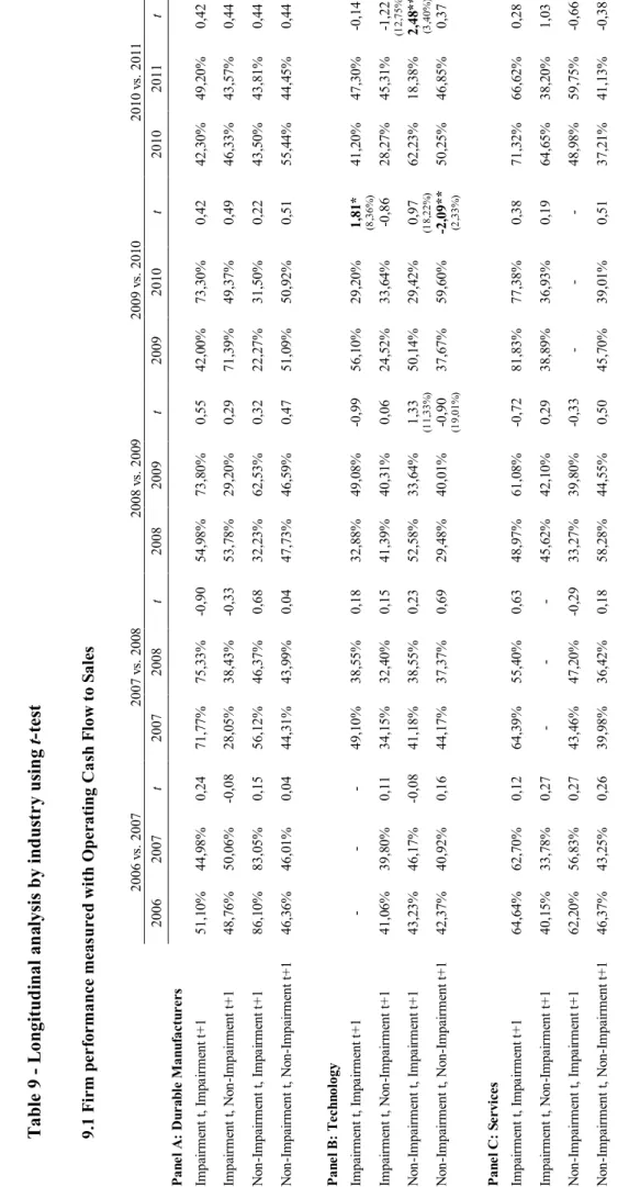
Table 9 - Longitudinal analysis by industry using t-test*... 47
Table 10 - Longitudinal global analysis using t-test* ... 50
Table 11 - Longitudinal analysis by industry using Wilcoxon Rank Sum test* ... 51
Table 12 - Longitudinal global analysis using Wilcoxon Rank Sum test*... 54
* This Table is divided in three Sub-Tables for each type of firm performance measure: Operating Cash Flow (Sub-Table 1); Earnings Before Taxes Excluding Unusual Items (Sub-Table 2); and Weighted Average of Operating Cash Flow and Earnings Before Taxes Excluding Unusual Items (Sub-Table 3).
CHAPTER 1
INTRODUCTION
The International Financial Reporting Standards 3 – Business Combinations (IFRS 3, 2008) defines goodwill as “an asset representing the future economic benefits arising from assets that are not capable of being individually identified and separately recognized”, being therefore obtained as the excess of the cost of an acquired entity over the fair value of its identifiable assets and liabilities.
Over time, goodwill has faced significant changes in terms of regulation (Ding et al., 2008). More recently, regulation tends to go in contradiction of goodwill amortization, by suggesting goodwill impairment tests in order to analyze the difference between the fair value of the reporting unit goodwill and the carrying amount of the correspondent goodwill.
In June 2001, the Financial Accounting Standards Board (FASB) firstly introduced this new concept, through the Statement of Financial Accounting Standards 141 – Business Combinations (SFAS 141, 2001) and the Statement of Financial Accounting Standards 142 – Goodwill and Other Intangible Assets (SFAS 142, 2001), under the framework of United States Generally Accepted Accounting Principles (US GAAP). Later in 2004, the International Accounting Standards Board (IASB) issued IFRS 3 (2004), under International Financial Reporting Standards (IFRS). In the same year, a revision occurred on the International Accounting Standards (IAS) through the International Accounting Standards 36 – Impairment of Assets (IAS 36, 2004) and the International Accounting Standards 38 – Intangible Assets (IAS 38, 2004). With the aim of moving towards international convergence, four years later, the FASB and the IASB revised SFAS 141 (2004) and IFRS 3 (2004), respectively, which resulted in SFAS 141 (2008) and IFRS 3 (2008).
The new accounting standards related to goodwill treatment, and particularly the replacement of systematic goodwill amortization by annual goodwill impairment tests, beget the question of subjectivity of the tests in evaluating goodwill impairment to recognize periodically. For instance, Churyk (2005) studied the appropriateness of the new standard issued in 2001 by testing market valuations of goodwill, finding weak evidence for the initial impairment of goodwill. Additionally, Devalle & Rizzato (2012) developed a study on the quality of the mandatory disclosure of IAS 36 (2004), with a particular focus on goodwill impairment disclosure, suggesting a low disclosure index and large discrepancies between the stock markets analyzed.
More specifically, in the context of the new rules introduced by SFAS 142 (2001), Vichitsarawong (2007) studied the usefulness of goodwill impairment by assessing the relative efficiency of companies, in the reality of the United States. Using a cross-sectional (comparison between firms) and a longitudinal analysis (comparison over time), the conclusions partially support the idea that goodwill impairment reflects the decrease in the relative firm efficiency. Consequently, the implementation of SFAS 142 (2001) contributes to the fulfillment of the FASB’s objective.
According to Swanson et al. (2013), although the main principles are similar, slight differences between the US GAAP and the IFRS approaches might suggest that it is easier for American companies using US GAAP to avoid incurring an impairment loss than for companies following IFRS principles. Therefore, results obtained when testing this possible relationship might end up being different with IFRS treatment, allowing the obtention of distinct conclusions. Moreover, periods of economic adversity are considered to be important moments for accounting regulation (Bertomeu & Magee, 2011). As a result, the incorporation of financial crisis years within the period of analysis may have an impact on results.
In this context, this dissertation aims at studying the same relationship developed by Vichitsarawong (2007), although concentrated on the European reality, taking the particular case of Germany, and considering a different and longer period of analysis. In fact, Germany is considered to be the largest economy in Europe, presenting the highest GDP over the past several years (Piirto, 2012). As a consequence of increasing integration in Europe, Germany’s commercial and accounting policies tend to be influenced by European Union regulation. Moreover, German culture plays an important role in the quality of accounting and reporting, since Germans reveal a tendency to be more conservative in the interpretation of probability expressions in the context of the IFRS (Doupnik & Richter, 2003).
Based on this, the present study attempts to give an answer to the following research question:
“How is goodwill impairment driven by relative firm performance? - Evidence from Germany”
Using different measures of firm performance for sensitivity analysis purposes, the hypotheses deriving from this research question are tested at two distinct dimensions. Firstly, a cross-sectional analysis intends to compare firms presenting goodwill impairments during
the period of analysis with others in the same industry but with no goodwill impairment recognition. Secondly, a longitudinal analysis aims to analyze the same relationship over time, individually for each firm.
The present paper contributes to current literature by applying the research study developed by Vichitsarawong (2007) to an European environment and to a subsequent and more extended period of time. Moreover, it discusses further managerial implications related to the topic, taking into consideration the findings from the statistical tests.
Besides, this analysis is particularly relevant for auditors, investors and other financial statement users since it helps to understand the usefulness of current accounting standards regarding goodwill recognition and impairment.
The remainder of this study is organized as follows. Chapter 2 presents the relevant accounting regulation on the topic. Chapter 3 reviews the related former literature. Chapter 4 is focused on the research question’s definition and develops the hypotheses. Chapter 5 contains the empirical study design, findings and managerial implications. Chapter 6 concludes the paper.
CHAPTER 2
ACCOUNTING REGULATION
This research study is focused on the goodwill impairment thematic in the context of the new accounting standards. For this purpose, a brief presentation of related accounting regulation is required. On the one hand, in the context of US-GAAP, the most important regulation about the topic is defined in SFAS 142 (2001). On the other hand, in the context of IFRS, IFRS 3 (2004; 2008) and IAS 36 (2004) are of extreme relevance.
2.1 SFAS 142 under US-GAAP
SFAS 142 (2001) refers to the financial accounting and reporting of acquired goodwill and other intangible assets, superseding the Accounting Principles Board Opinion 17 - Intangible Assets (APB Opinion 17, 1970). According to this standard, the need for the issue of the new statement arose partly in response to financial statements users’ opinion, arguing the usefulness of goodwill amortization in analyzing investments. Changes introduced by the statement intend to improve financial reporting by offering a better understanding of the underlying economic value of goodwill and consequently allowing users to better evaluate companies’ future profitability and cash flows (SFAS 142, 2001, Summary).
Paragraph 19 of SFAS 142 (2001) states that goodwill shall not be amortized, but instead tested for impairment. The impairment exists when the value of the carrying amount of goodwill is higher than the implied fair value. According to this standard, goodwill should be tested by managers at the reporting unit level. A reporting unit level is defined in paragraph 10 of the Statement of Financial Accounting Standards 131 – Disclosures about Segments of an Enterprise and Related Information (SFAS 131, 1997) as an operating segment or one level below an operating segment. A two-step impairment test must be followed.
1. The first step of the goodwill impairment test is concentrated on identifying potential impairment. For that, a comparison between the carrying amount and the fair value of a reporting unit1 (including goodwill) should be made. If the fair value of a reporting unit is higher than its carrying amount, no impairment should be recognized. However, if the carrying amount of a reporting amount is higher than its fair value, one should proceed to the second step in order to measure the amount of impairment of goodwill to recognize.
2. The second step of the impairment test is focused on evaluating the value of goodwill impairment to recognize. In this case, the implied fair value of reporting unit goodwill2 and the carrying amount of that goodwill should be compared. If the carrying amount of reporting unit goodwill is higher than the implied fair value of that goodwill, the amount of the excess should be recognized as an impairment loss. From that time, the new accounting basis of the goodwill will be the adjusted carrying amount of the goodwill.
In general, impairment tests should be made annually. Nevertheless, under certain circumstances, additional impairments might be necessary, as the example of considerable legal adverse changes; adverse changes in the business environment; adverse actions by regulators; unexpected competition; and others.
Under these norms, one should notice that, not only management estimates and assumptions in impairment testing are subjective, but also information concerning each reporting unit is frequently difficult to obtain (Vichitsarawong, 2007).
Furthermore, during the process of determining goodwill impairments, managers make use of present value techniques to measure the fair value of a reporting unit. However, future cash flows estimate is based on past and present performance, evidencing the relevance of firm performance in assessing a goodwill impairment loss (Vichitsarawong, 2007).
1
According to paragraph 23 of SFAS 142 (2001), “the fair value of an asset (or liability) is the amount at which that asset (or liability) could be bought (or incurred) or sold (or settled) in a current transaction between willing parties...” “If quoted market prices are not available, the estimate of fair value shall be based on the best information available, including prices for similar assets and liabilities and the results of using other valuation techniques.”
2
In accordance with paragraph 21 of SFAS no. 142, “the implied fair value of goodwill should be determined in the same manner as the amount of goodwill recognized in a business combination is determined.” “The excess of the fair value of a reporting unit over the amounts assigned to its assets and liabilities is the implied fair value of goodwill”.
2.2 IFRS 3 and IAS 36 under IFRS
Issued by the IASB, IFRS 3 (2008) was developed with the aim of improving the “relevance, reliability and comparability of the information” delivered by a reporting entity in its financial reporting concerning “business combinations and its effects” (IFRS 3, 2008, Objective). IAS 36 (2004) develops the subject of impairment of assets, stating that goodwill should be subject to impairment tests on an annual basis or more frequently in certain circumstances. The standard demands acquired goodwill in a business combination to be tested for impairment in the context of the impairment testing the cash-generating unit(s) is associated with. The cash-generating units to which goodwill is allocated should present the lowest level of entity to which goodwill is assigned. Furthermore, the unit or group of units to which the goodwill is allocated should not be larger than an operating segment. Under IAS 36 (2004), the recognition of impairment occurs when the carrying value of the cash-generating units is higher than the greater value of its value in use and its net realizable value (i.e., its recoverable amount).
Although one of the main purposes of the changes in IFRS 3 (2004) was related to the convergence intention with US GAAP, some differences still remain between the two accounting treatments, according to Jerman & Manzin (2008).
Firstly, concerning the cash-generating units (or reporting units), SFAS 142 (2001) do not allow a reporting unit to be identified at a lower level than an operating segment, while IAS 36 (2004) does not establish such constraint. Consequently, under IFRS the impairment test may be done at a lower level when comparing to US GAAP.
Secondly, there is a significant difference regarding the impairment testing of goodwill. The approach followed by IAS 36 (2004) does not suggest a two-step method, meaning that the impairment loss should be calculated at the moment of the conclusion of step number one. These differences might suggest that is easier for American companies using US GAAP to avoid incurring an impairment loss than for companies following IFRS principles (Swanson et al., 2013). According to the authors, this may happen because reporting units may be softened and restructured in a way that fair market values of the reorganized units do not present losses at an individual level. Also, cash-generating units require assets or groups of assets to be linked to certain cash flows, which have no relation to the other cash flows of the company. Hence, it would be more unlikely to avoid impairment losses recognition when there is an indication of the deterioration of the specific assets.
CHAPTER 3
LITERATURE REVIEW 3.1 Goodwill impairment
After presenting the accounting regulation associated with the topic, it is important to explain the background of goodwill treatment over time. Given the recent modifications introduced by new accounting standards, prior literature on the value relevance of goodwill impairment is examined.
3.1.1 Goodwill treatment over time
IFRS 3 (2008) defines goodwill as “an asset representing the future economic benefits arising from assets that are not capable of being individually identified and separately recognized”, being therefore obtained as the excess of the cost of an acquired entity over the fair value of its identifiable assets and liabilities. The value of goodwill is created from the value of combining entities, being related to improvements of management efficiency (Lang et al., 1989), synergies gains resulting from economies of scale (Bradley et al., 1988) and benefits from internal financial advantages in comparison to external financing (Nielsen & Melicher, 1973). Also, goodwill may result from the integration of processes, enhancement of production techniques (Vichitsarawong, 2007). Therefore, goodwill represents an important portion of a firm’s value. For instance, during the period from 1990 to 1994, it represented approximately 20 percent of the overall assets of business combinations (Henning et al., 2004).
Over time, goodwill has faced significant changes in terms of regulation. Ding et al. (2008) considers four main phases in the evolution of goodwill treatment, in the period between 1985 and 2005 and focusing the analysis on four Western capitalist countries: Germany, Great Britain, United States and France.
The first phase is mentioned as the static phase (non-recognition phase), arguing that goodwill is considered a true asset and therefore it should be expensed, instantaneously or within a short period of time. The second stage is referred to as the weakened static phase, in which goodwill is charged as equity, combining two distinct arguments: firstly, goodwill is not an asset; secondly, it should give the opportunity of dividend distribution from the current profit.
Phase number three is the dynamic phase, claiming that acquired goodwill should be systematically amortized in a way that reduces current income. Particularly, APB Opinion 17 (1970) required for goodwill to be amortized over a period that could not exceed 40 years, while the previous International Accounting Standards 22 – Business Combinations (IAS 22, 1998) imposed a linear amortization that could not exceed 20 years (Jerman & Manzin, 2008). Finally, the fourth phase is named as the actuarial phase and goes against goodwill amortization, by suggesting goodwill impairment tests in order to analyze the difference between the fair value of goodwill and the carrying amount of the correspondent goodwill. In 2001, the FASB firstly introduced this new concept, through SFAS 141 (2001) and SFAS 142 (2001), under the framework of US GAAP. Later in 2004, the IASB issued IFRS 3 (2004), under IFRS. In the same year, a revision occurred on the IAS through IAS 36 (2004) and IAS 38 (2004). With the aim of moving towards international convergence, four years later, the FASB and the IASB revised SFAS 141 (2004) and IFRS 3 (2004), respectively, which resulted in SFAS 141 (2008) and IFRS 3 (2008).
Considering the particular case of Germany, Ding et al. (2008) mentions the first phase has being deemed to occur between 1880 and 1985; the second one from 1985 to 2000; the third one between 2000 and 2005 and finally the current stage from 2005 onwards. This year corresponds to the period in which preparation of consolidated financial statements under IFRS became mandatory for European Union listed companies.
3.1.2 Value relevance of goodwill impairment
The elimination of systematic goodwill amortization, giving place to annual goodwill impairment tests, brings the question of the value relevance of goodwill impairment, as a result of the uncertainty and subjectivity of the tests in evaluating goodwill impairment to be recognized periodically.
Churyk (2005) studied the appropriateness of the new standard issued in 2001 by testing market valuations of goodwill, finding weak evidence for the initial impairment of goodwill, but strong support for the following impairments.
Devalle & Rizzato (2012) develops a study on the quality of the mandatory disclosure of IAS 36 (2004), with a particular focus on goodwill impairment disclosure. The results suggest a low disclosure index and large discrepancies between the stock markets analyzed.
In another empirical study, Xu et al. (2011) analyzes the value relevance and reliability of reported goodwill impairment and concludes that, while typically regarded as relevant information, the signal delivered depends on the profitability of the firm. Thus, regarding goodwill impairment recognition, in the case of profitable firms there is a negative connotation developed by investors, while for unprofitable companies this negative signal does not exist. In this context, it seems to be advantageous to evaluate and disclose goodwill impairment on an annual basis.
Some studies have suggested that decisions regarding goodwill might be affected by specific external variables. For instance, Detzen & Zülch (2012) explores the relationship between CEO’s short-term cash bonuses and the amount of goodwill recognized in IFRS acquisitions. The findings indicate that increasing cash bonus for managers have a positive impact on the amount of goodwill recognized.
Also, and specifically in line with subject of this study, the decision regarding impairment of goodwill may be affected by certain factors. Masters-Stout et al. (2008) studied the tenure of the chief executive officer and the his/her goodwill impairment decisions, concluding that managers in charge will tend to recognize a greater amount of goodwill impairment in the first years with two possible aims: first, blaming previous managers on decisions regarding acquisitions; secondly, increasing future earnings by expensing goodwill at a earlier stage. Finally, Guler (2007) finds out that managers’ reporting incentives affect their decision to recognize impairments of goodwill. In addition, there seems to exist a relationship between the recognition of goodwill impairment losses and the strength of the firm’s corporate governance.
3.2 Firm performance
Firm performance, and particularly firm performance measurement, is a subjective topic and therefore may be evaluated considering distinct variables and dimensions. In fact, this topic has been a concern in strategic management research for many years (Zimmerman, 2001; Chakravarthy & Jones, 1986).
Some authors argue that the main concern related to firm performance is a gap between the “specification of the firm performance construct and the way performance is measured in empirical research study” (Glick et al., 2013). As a result, it may be complicated to establish a
comparison between the findings of researches that are based on the same theoretical concepts, although using distinct performance measures (Steigenberger, 2014). Some variables may be better than others and as a result the merits and demerits of particular measures and types of measures of firm performance have been examined over the years (Dalton & Aguinis, 2013; Richard et al., 2009).
According to Lau (2011), performance measures may be classified as financial and nonfinancial. Particularly in what concerns to financial measures, these are the type of measures, as the example of cash flows and profits, that may be aggregated and compared across firms (Meyer, 2002).
It is certainly useful providing a brief compilation of financial measures used in previous studies. Firstly, Francis et al. (1996) relies on changes in return on assets to control for firm performance, defining return on assets as the ratio of income before extraordinary items to average total assets. Secondly, the percent change in sales for firms from prior year may be a way of measuring firm performance (Riedl, 2004). Thirdly, Păşcan & Ţurcaş (2012) measures the impact of first-time adoption of IFRS on the performance of Romanian groups of listed companies, being performance expressed by means of net income. Lastly, Park & Jang (2013) studies the relationship between capital structure, free cash flow, diversification and firm performance, measuring the latter using Tobin’s q, a measure of firm assets in comparison to the firm’s market value.
More specifically, Delen et al. (2013) explores the evaluation of performance using financial ratios. The authors argue their advantage in terms of establishing comparisons across companies in the same industry, between industries, or even within an enterprise itself. These tools also allow for the comparison of relative performance for companies of different size. An empirical study led to the conclusion that firm performance, represented as return on equity or return on assets, is mainly impacted by three types of ratios. Firstly, the profitability ratios are considered, more specifically earnings before tax-to-equity ratio and net profit margin. Secondly, leverage and debt ratios were found to have an impact on performance. Lastly, the importance of sales growth and asset turnover rate as measures of the company’s ability to generate sales and consequently impact the overall performance was highlighted. From a different point of view, Coelli (2005) considers efficiency as a possible measure of performance. Considering inputs used by a firm and outputs obtained by the same, the author defines efficiency as a ratio of the significant outputs to the considerable inputs. Also Neely et al. (1995) defines a performance measure as a “metric used to quantify the efficiency and/or
effectiveness of action”. Based on this, Vichitsarawong (2007) uses efficiency as a measure of financial performance, considering cost of goods sold; selling, general and administrative expenses; current assets; fixed assets; and intangible assets as inputs and sales; income before extraordinary items; and operating cash flows as outputs. For the author, performance is a relative concept (relative efficiency), being always evaluated in comparison to the performance of another company or to the performance of the same company but relative to a different period of time.
3.3 Goodwill impairment and relative firm performance
In theory, goodwill represents the present value of a combination of expected future cash flows and for that reason it is recorded as an asset (Jennings & Robinson, 1996). Nonetheless, cash flows associated with goodwill will be mixed with those related to other assets owned by the company. As a consequence, goodwill impairment is expected to indicate a signal of relevant changes in the value of goodwill and expected company’s future earnings (Hirschey & Richardson, 2002).
Having this in mind, and in the context of the new rules introduced by SFAS 142 (2001), Vichitsarawong (2007) studied the usefulness of goodwill impairment by assessing the relative efficiency of companies, in the reality of the United States. Using a cross-sectional (comparison between firms) and a longitudinal analysis (comparison over time), the conclusions showed that goodwill impairment reflects the decrease in the relative firm efficiency and consequently the implementation of SFAS 142 (2001) allows the achievement of the FASB’s objective. Additionally, the author studies the role of the relative efficiency of firms in the decision to recognize goodwill impairment charges, as well as in the definition of the quantity of goodwill impairment, for the reality of the United States. The results confirm that relative efficiency is an important determinant of goodwill impairment.
3.4 The German reality
Germany is considered the largest economy in Europe, presenting the highest GDP in the past several years (Piirto, 2012). It is seen as a stakeholder economy, although with a less-developed stock market, lack protection for investor and concentrated ownership (La Porta et
al., 1998; Leuz & Wüstemann, 2003). German accounting standards are the Germany Generally Accepted Accounting Principles (German GAAP) follow the HGB, the commercial code in Germany, in which financial reporting and auditing regulations are dependent on the legal form (Brown et al., 2013).
As a consequence of increasing integration in Europe, Germany’s commercial and accounting policies tend to be influenced by European Union regulation. Also the German culture plays an important role in the quality of accounting and reporting, since Germans reveal a tendency to be more conservative in the interpretation of probability expressions in the context of the IFRS (Doupnik & Richter, 2003).
However, IFRS is less important in Germany when comparing to other countries, as the example of United Kingdom. This happens because, although IFRS have been focused on investors’ interests and needs, a great number of German firms are privately owned and only capital market companies are obliged to apply IFRS for their consolidated financial statements (Hellmann et al., 2010). In fact, the accounting policies for individual financial statements of the companies mostly follow the HGB. In accordance to Hellmann et al. (2010), there have been some inconsistencies in the application of IFRS, which may be related to several causes: the fact that financial statements in Germany might be prepared by accountants who may not be associated with a professional entity; translation of IFRS into German; interpretation of IFRS by Germans; lack of quality accountants, education and training; and lobbying activities.
CHAPTER 4
RESEARCH QUESTION AND HYPOTHESES DEVELOPMENT 4.1 Research question
A previous study developed by Vichitsarawong (2007) attempted to establish a relationship between goodwill impairment and relative efficiency of firms in order to determine the usefulness of goodwill impairment under SFAS 142 (2001). Similarly, this research intends to study the relationship between goodwill impairment and firm performance, although using a distinct environment and considering a subsequent and more extended period of analysis. Therefore, instead of focusing the analysis on the United States market following US-GAAP, this research will be concentrated on the European reality under IFRS, taking the particular case of Germany. According to Swanson et al. (2013), although the main principles are similar, slight differences in the US GAAP and IFRS approaches might suggest that is easier for American companies using US GAAP to avoid incurring an impairment loss than for companies following IFRS principles. Hence, the results obtained when testing this possible relationship might end up being different with IFRS treatment, allowing therefore to obtain distinct conclusions.
Despite the fact that IFRS is less important in Germany when comparing to other European countries (Hellmann et al., 2010), this country is considered the largest economy in Europe (Piirto, 2012) and consequently an adequate representation of the European reality. Also, only companies of this country are chosen in order to obtain stable environments.
In addition, periods of economic adversity are considered to be important moments for accounting regulation (Bertomeu & Magee, 2011). Kousenidis et al. (2013), basing their analysis in the countries more affected with the financial crisis, suggests that, although earnings quality has improved in the crisis period, there is still a deterioration of reporting quality if there are incentives for earnings management. This way, the incorporation of financial crisis years on the period of analysis may have an impact on the results obtained. Having all the previous ideas into consideration, this research is focused on the topic of the goodwill impairment in the context of the new accounting standards and attempts to give an answer to the following research question: “How is goodwill impairment driven by relative firm performance? – Evidence from Germany”. The theoretical approach is presented in Figure 1.
Figure 1 - Theoretical model
Goodwill: “asset representing the future economic benefits arising from assets that are not capable of being individually identified and separately recognized” (IFRS, 2008)
Cash flows associated with goodwill will be mixed with those related to other
assets owned by the company (Hirschey, 2002)
In case there is a goodwill impairment, it means companies are using economic resources in a less efficient way (Vichitsarawong, 2007)
When comparing to firms with no goodwill impairment recognition
When comparing to years of no goodwill impairment recognition
Consequently, there is an expectation of lower relative firm performance (Vichitsarawong, 2007)
4.2 Hypotheses development
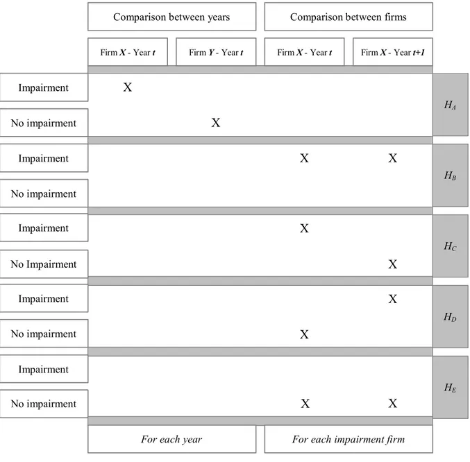
In order to give response to the research question, two distinct analyses are developed, based on five hypotheses that are presented below.
4.2.1 Cross-sectional analysis
Since cash flows associated with goodwill will be mixed with those related to other assets owned by the company, goodwill impairment is expected to indicate a signal of relevant changes in the value of goodwill and expected company’s future earnings (Hirschey & Richardson, 2002).
Like Vichitsarawong (2007), this study will begin to develop a cross-sectional analysis, based on the hypothesis that impairment firms tend to use their economic resources in a less efficient way when comparing to non-impairment companies. As a consequence, impairment firms are expected to present lower performance, lower profitability and lower net cash flows. Based on this reasoning, the first alternative hypothesis uses both impairment and non-impairment firm samples and is defined below:
HA: Impairment firms present relative low performance than non-impairment firms in the year of goodwill impairment recognition.
4.2.1 Longitudinal analysis
Also similarly to Vichitsarawong (2007) the longitudinal analysis aims at studying changes in the relative firm performance of impairment and non-impairment firms over time. Based on the reasoning that firms are more likely to present lower firm performance in the years of goodwill impairment recognition, four scenarios are considered.
The first hypothesis is focused on the study of the relationship of goodwill impairment and relative firm performance for the case of companies that, in two consecutive years, present impairment losses on both years. In this event, it is expected a decrease in firm performance from one year to the other. The definition of the alternative hypothesis is therefore defined as follows:
HB: If impairment firms report goodwill impairment in two consecutive years, firm performance is higher in the first year (of impairment reporting) comparing to the second year (of impairment reporting).
The second case aims to cover the situations in which a firm recognizes goodwill impairment in a first year, although in the second year there is no recognition related to this subject. Once again, it is expected that in the year of goodwill impairment recognition the performance is lower. The alternative hypothesis is therefore the following:
HC: In two consecutive years, if firms report goodwill impairment in the first year but not in the second year, firm performance is lower in the first year (of impairment reporting) comparing to the second year (of no impairment reporting).
On the contrary, it might occur the inverse case, assuming no impairment in the first year of analysis, but impairment recognition in the following year. Applying the same reasoning, the alternative hypothesis should be defined as follows:
HD: In two consecutive years, if firms report goodwill impairment in the second year without having reported in the first year, firm performance is higher in the first year (of no impairment reporting) comparing to the first year (of impairment reporting).
Finally, the case that is lacking consideration is the one in which there are no impairment losses during two consecutive years. This situation may suggest that performance has increased from one year to the other, otherwise a goodwill impairment loss should have been recognized in the second year. This way, the last alternative to consider is presented below:
HE: If impairment firms do not report goodwill impairment in two consecutive years, firm performance is lower in the first year (of no impairment reporting) comparing to the second year (of no impairment reporting).
Figure 2 - Hypotheses development scheme
X
Comparison between firms Comparison between years
X
X
X
No impairmentX
X
X
X
X
No impairment HD Firm X - Year t HA Impairment No impairment HC HB Impairment No impairmentFirm Y - Year t Firm X - Year t Firm X - Year t+1
Impairment No Impairment Impairment
X
Impairment HEFor each impairment firm For each year
CHAPTER 5 EMPIRICAL STUDY 5.1 Data and sample selection
The data and sample selection process starts with the compilation of the list of equity and/or debt publicly traded companies in Germany present in the Directory of Public Companies in Germany by the Credit Risk Monitor and belonging to three specific industries: durable manufacturing industry, technology industry and service industry.
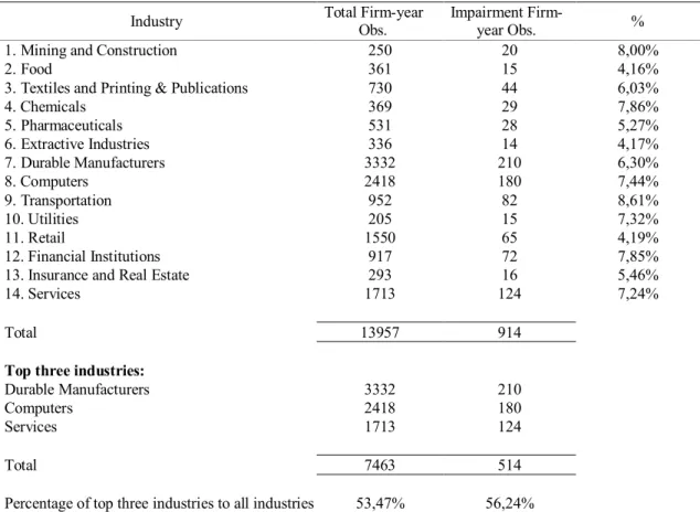
The choice of the three industries is based on the relevance of mergers and acquisitions activity and the frequency of goodwill impairment losses recorded for each industry (Vichitsarawong, 2007). In fact, the same author provided 514 firm-year observations with goodwill impairment losses belonging to the top three industries, representing approximately 56 percent of the overall observations from the 14 industries considered (Table 1).
Table 1 - Industry distribution of impairment observations (2002-2005) Industry Total Firm-year
Obs.
Impairment
Firm-year Obs. %
1. Mining and Construction 250 20 8,00%
2. Food 361 15 4,16%
3. Textiles and Printing & Publications 730 44 6,03%
4. Chemicals 369 29 7,86% 5. Pharmaceuticals 531 28 5,27% 6. Extractive Industries 336 14 4,17% 7. Durable Manufacturers 3332 210 6,30% 8. Computers 2418 180 7,44% 9. Transportation 952 82 8,61% 10. Utilities 205 15 7,32% 11. Retail 1550 65 4,19% 12. Financial Institutions 917 72 7,85%
13. Insurance and Real Estate 293 16 5,46%
14. Services 1713 124 7,24%
Total 13957 914
Top three industries:
Durable Manufacturers 3332 210
Computers 2418 180
Services 1713 124
Total 7463 514
Percentage of top three industries to all industries 53,47% 56,24% Source: Vichitsarawong (2007)
Based on this, the present study considers three industries. Firstly, durable manufacturer industry comprises chemical manufacturing; construction services; consumer cyclical; containers & packaging; fabricated plastic & rubber; miscellaneous capital goods; miscellaneous fabricated products; and non-metallic mining. Secondly, technology industry covers computer networks; computer peripherals; computer services; and extends further in the industry to communication services; communications equipment; electronic instruments and controls; semiconductors; and software & programming. Thirdly, service industry encompasses a wide variety of businesses: advertising; broadcasting & cable TV; business services; communications services; motion pictures; personal services; real estate operations; printing & publishing; restaurants; retailing, utilities; recreational activities; transportation; and hotels & motels.
Using Capital IQ as the source for data collection, an initial sample of 675 firms for the fiscal years from 2006 to 2011, presenting goodwill balances under IFRS, is obtained.
The next step requests an elimination of companies with no goodwill impairment during the period of analysis - 464 firms - and also companies presenting missing data (for instance, absence of information regarding one specific financial statement) – 123 firms. At this point, the final sample comprises a total number of 88 firms, composed of 33 durable manufacturing firms, 29 technology firms and 26 service firms. These are named impairment firms and consist of firms with goodwill impairment losses for at least one year during the period between 2006-2011.
All these firms are tested under the longitudinal analysis regarding the different hypotheses previously presented.
However, the cross-sectional analysis requires some adjustments concerning the size of the company, in order to eliminate the presence of outliers that may bias the analysis. In that sense, the cross-sectional samples should only include companies presenting an average of total assets (considering the six years of analysis) between one billion euros and 2000 billion euros. Consequently, the sample is reduced to a total amount of 63 firms (22 durable manufacturing firms, 27 technology firms and 14 service firms).
In addition, for the special purpose of the cross-sectional analysis, a control sample of firms is collected, using 63 firms (22 durable manufacturing firms, 27 technology firms and 14 service firms), which report goodwill on the balance sheet, but no goodwill impairment losses over the period of analysis. These are named non-impairment firms and are selected randomly
within the list of sample firms fulfilling the requirements. Once obtained, this is the sample whose firms’ performance is to be compared to that of impairment firms.
The complete list of sample firms, containing both impairment and non-impairment firms, is presented on Exhibit 1 and the entire data and sample selection process is presented in Table 2.
Table 2 - Sample selection
Selection Procedure Firm-year
Observations Available observations for Germany public companies with goodwill balances from IQ
Capital database between 2006-2011 for durable manufacturer, technology and service industries
675
Observations deleted due to:
- No goodwill impairment 464
- Missing data 123
Final sample 88
Longitudinal analysis:
Impairment observations classified by industry:
- Durable manufacturers 33
- Technology 29
- Services 26
Total sample 88
Adjustments for the cross-sectional analysis due to:
- No match with size requirements (total assets between €1 billion and €2000 billion) 25 Cross-sectional analysis:
Impairment observations classified by industry:
- Durable manufacturers 22
- Technology 27
- Services 14
Total sample 63
Note: For the cross-sectional analysis, the final impairment sample is matched with firms that present no goodwill impairment during the period of analysis, named non-impairment firms, presenting similar size (in terms of total assets) and available data for the same period of time.
5.2 Variables for firm performance measurement
The previous Chapter 3.2.2 supports the idea that firm performance measurement is a subjective topic and therefore it may be evaluated considering distinct variables and dimensions.
Based on the approach followed by Delen et al. (2013), this study makes use of financial ratios to measure performance, taking into account the purpose of comparing companies in
the same industry and across industries. Similarly, such ratios are also suitable when comparing companies with significantly disparate sizes. In that sense, all initial variables are divided by total sales in order to normalize the results and isolate scale effects.
Furthermore, the argument from Steigenberger (2014), based on the idea that conclusions from a study may differ according to the performance measures used, further reinforces the importance of evaluating more than one variable in the statistical analysis.
While measuring relative efficiency, Vichitsarawong (2007) considers as output variables three distinct measures: sales, income before extraordinary items3 and operating cash flow. Similarly, this research follows a relative approach, by considering the percentile ranks of each observation in relation to the overall observations of the industry. In addition, with the objective of developing a sensitivity analysis to the firm performance measurement, three distinctive ratios are considered in this research:
Operating Cash Flow to Sales: this is a standard item shown in the cash flow statement of each firm, and collected within the Capital IQ database. It is important to mention that this particular database uses the indirect method to calculate operating cash flow, adjusting net income from the income statement for the effects of non-cash transactions. Moreover, it provides the operating cash flow including interest expenses (which are assumed to be related to the operational activity). This is permitted under IFRS, according to the International Accounting Standards 7 – Statement of Cash Flows (IAS 7, 2007), paragraph 31, in the case that interest expenses are paid regularly and there is no discretion.
Earnings Before Taxes Excluding Unusual Items to Sales: similarly, this is a standard item presented in the Capital IQ database, in the income statement of each company. In a simplified way, this can be interpreted as the amount of money earned by a firm, after the cost of goods sold, interest expenses and operating expenses have been deducted from gross sales. This also excludes unusual items, such as restructuring changes, gain/loss on sale of assets, asset write-down and, notably, impairments of goodwill. Logically, for the purpose of this dissertation, the effect of the last item should not be considered.
Equally Weighted Average of the two variables mentioned above (Operating Cash Flow to Sales and Earnings Before Taxes Excluding Unusual Items to Sales): to improve the robustness of the results obtained, the third measure results from a combination of the two previous variables, with a weight of 50 percent each.
3
Regarding these two specific variables, Miller et al. (1988) argues that many managers have preferred evaluation techniques relying on cash flows rather than the ones based on profits. The main reason is related to the fact that cash in and cash equivalents is what can be actually spent or invested, and not the accounting figures such as profits based on an accrual assessment. Following this reasoning, cash flow is the most appropriate measure to pay attention to.
Finally, one should notice that both measures reflect the effect of capital structure, which may have an impact on the results obtained. However, as the performance of each firm is always measured relatively to the performance of the firms in the same industry, significant differences in terms of leverage decisions are not expected. As a matter of fact, Kayo & Kimura (2011) states that “firms working in the same industry present similar behavior regarding financial decisions, although such patterns differ across industries.”
5.3 Methodology
According to Wijnand & Velde (2000), there are different statistical tests that can be used in order to analyze if two samples come from the same distribution. The null hypothesis assumes that there is no systematic difference between two different samples and therefore they come from the same distribution. Conversely, the alternative hypothesis undertakes a systematic difference between the two samples. In case the test results in a considerably large probability that samples derive from the same distribution, the null hypothesis is not rejected. If, on the other side, the test leads to a small probability, the null hypothesis is rejected and the difference is consequently said to be statistically significant at a certain percentage level. The p-value indicates the probability that a test statistic is at least as extreme as the one computed, assuming that the null hypothesis is true (Goodman, 2008).
Assuming the distribution follows a normal distribution, it is common to use a parametric test, named two-sample t-test. However, in case the underlying distribution is not normal and specifically in the case of smaller samples, a non-parametric two-sample test, such as the Wilcoxon Rank Sum test, may be a suitable alternative (Wijnand & Velde, 2000).
In past literature there is not a consensus about which type of test is preferred over the other. For instance, Norman (2010) argues that parametric tests are appropriate for Likert data, small sample sized, unequal variances and non-normal distributions, with no risk of obtaining erroneous conclusions. Though, other authors argue that, in the absence of normality or
chance to induce normality in a suitable way, non-parametric tests may bring advantages such as higher relative efficiency.
Therefore, for the purpose of the hypotheses of this study, and considering that the sample sizes are relatively small, both type of tests are conducted – a t-test and a Wilcoxon Rank Sum test. In this context, it is possible to increase the robustness of the results obtained, by comparing findings and conclusions derived from both methodologies. All statistical tests are developed manually using Excel tools.
5.3.1 t-test
In order for a t-test to be considered valid, four requirements must be satisfied: independence of observations, inexistence of outliers, homogeneity of variances and normally distributed data (Osborne et al., 2012).
Regarding the independence of observations, each firm’s observation is independent from the others’ (in the cross-sectional analysis) and the firm’s observation in one specific year is not related to the observation in the previous or following year (in the longitudinal analysis). In that sense, the same observations are not present in the two groups of analysis simultaneously. The inexistence of outliers could be more critical in the cross-sectional analysis, as in the longitudinal analysis the observations belong to the same firm. However, this condition is met with the size requirement for the cross-sectional sample (comprising only firms with a total average of assets between 1 billion euros and 2000 billion euros – see Table 2), which eliminates the presence of possible outliers.
In what concerns to the homogeneity of variances, there is no indication that the variance of the observations is significantly different from sample to sample, as the analysis is always performed taking into consideration the relative firm performance within the same industry. Finally, the normality condition is assumed to be true through the use of percent ranks taking the industry as reference. Nonetheless, a sensitivity analysis is presented afterwards, through a non-parametric test.
Assuming the previous requirements are met, a t-test on the mean differences of relative firm performance of the samples is performed, for each of the hypotheses.
5.3.2 Wilcoxon Rank Sum test
For the Wilcoxon Rank Sum test to be valid, only two assumptions are required: that samples are random from their respective populations and that observations are independent from each other (Wijnand & Velde, 2000).
Despite the fact that impairment firm samples are mainly selected from the list of public companies in Germany subject to size requirements and information availability in the IQ Capital database, random samples may be assumed, as the sample used considerably represents the overall population of Germany firms presenting goodwill impairments under IFRS. Additionally, the list of non-impairments firms is randomly selected among the list of available firms in order to meet the number of impairment firms previously collected.
Concerning the independence of the samples, the justification presented in the t-test approach may be applied.
Using this methodology, the original elements are ranked by numbers. In this particular two-sample test, the procedure is to combine the two two-samples into a single and combined ordered sample, regardless of which population each observation belongs to and attributing rank numbers from the smallest to the largest value. The next step is to obtain the sum of the rank numbers of one sample. This essentially systematizes the intuition according to which a large rank sum may suggest that the values from that population are probably higher than the values belonging to the other population. Naturally, a small rank sum should lead to an opposite conclusion (Wijnand & Velde, 2000).
This statistical test is particularly useful for the longitudinal analysis, as sample sizes for each of the hypotheses are smaller, most of the times lower than ten.
5.4 Results and findings
Results and findings are presented separately for each type of analysis: Sub-Chapter 5.4.1 develops cross-sectional analysis and Sub-Chapter 5.4.2 is focused on the longitudinal analysis. The tables concerning each type of analysis are shown in the end of each Sub-Chapter.
5.4.1 Cross-sectional analysis
In order to study the first hypothesis, a sample of both impairment and non-impairment firms is considered.
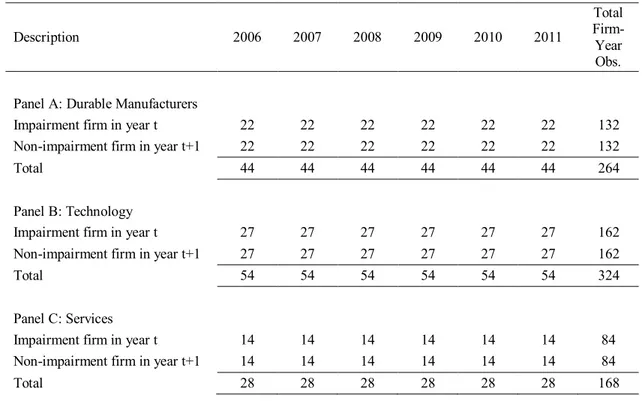
Table 3 presents the sample distribution by industry. Due to companies’ data availability, the number of companies for each industry is slightly different. Therefore, technology industry (Panel B) is the one presenting a higher number of companies, with 54 entities (both impairment and non-impairment firms) in each year, totaling 324 data points during the entire period. The second larger sample encompasses the durable manufacturer industry (Panel A), with a total of 264 data points during the six years, which represents 44 companies per year. Finally, services (Panel C) are the industry with the smaller sample size, since only 28 firms are analyzed each year, accounting for a total number of 168 data points over the six-year period.
Tables 4 to 7 summarize the results of the cross-sectional analysis, divided by type of statistical test and type of performance measure.
More specifically, Table 4 presents the t-test results used to analyze the difference of relative performance means for impairment and non-impairment firms, for different types of performance measures and evaluating each panel individually.
Using a left-tailed test, the null hypothesis assumes no difference in the companies’ performances, while the alternative hypothesis assumes companies with goodwill impairment losses present a relative lower performance when comparing to non-impairment firms.
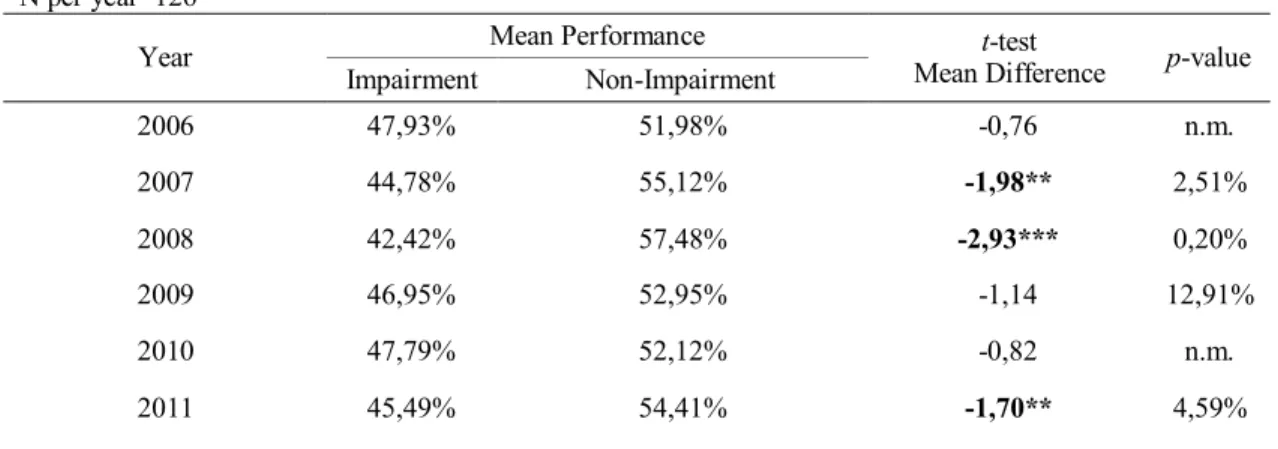
Table 4.1 shows the results assessing firm performance based on the Operating Cash Flow to Assets ratio. In general, all the industries present negative mean differences between impairment firms’ relative performance and non-impairment firms’ relative performance, across the entire period of analysis (with the exceptions of durable manufacturers in 2009 and 2010 and services in 2006). However, the only industry presenting statistically significant mean differences is the technology industry. Excluding the years of 2006 and 2010, the mean differences of relative firm performance are statistically different from zero in each year, at least at a 10% level. The most significant difference occurs in the year of 2008, with a p-value of 0,27%.
Table 4.2 considers a different measure of firm performance, Earnings Before Taxes Excluding Unusual Items to Assets ratio. In this case, the results show again negative mean differences in both durable manufacturer and technology industries, although this difference
tends to be positive in the case of the service industry (t-test is always above 6), going against the prediction. Once again, the only significant results are the ones related to the technology industry.
Finally, Table 4.3 uses an equally Weighted Average of the two measures presented above. Considering both measures simultaneously, the results strongly support the hypothesis for the technology industry, although there are no significant differences in the conclusions for the other two industries.
The differences of results in terms of industries may possibly be explained by the different sample sizes. In that sense, technology industry comprises the largest sample and therefore presents a greater amount of significant results. By contrast, service industry presents a few significant results and these are quite contrasting according to the type of performance measure used. As a matter of fact, this industry in not only the one presenting the smallest sample, as it also includes a wide variety of businesses with different particularities (the sample includes firms from advertising, communication, entertainment, retailing, and others). Taking this into consideration, less robust results may be expected from the service industry. Table 5 shows the results of an aggregate analysis, by applying the same tests to a sample including the three industries’ samples at the same time, resulting in a total of 126 firms in each year and, consequently, 756 data points over the entire period. In this case, there are significant results when performance is measured using the cash flow statement item, and also when using the weighted average measure. The significance of these results may probably arise from the larger sample size. Conversely, the income statement item measure is the less supportive of the hypothesis, given that results are never significant and the t-test mean difference is, in most cases, even positive.
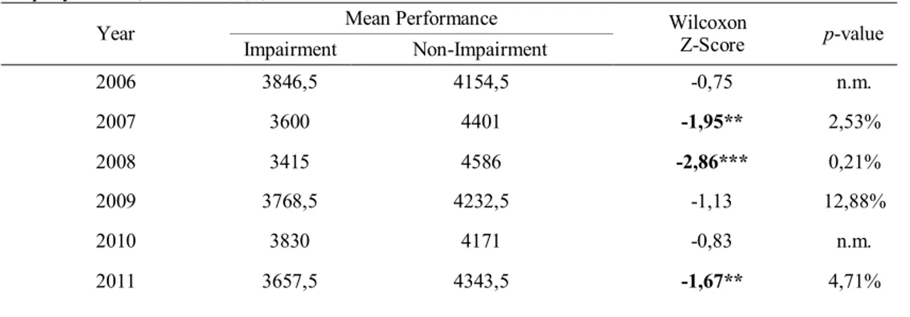
With the aim of increasing the robustness of results, an alternative statistical test is developed - a non-parametric test named Wilcoxon Rank Sum test. However, one should mention that, for this particular analysis, as sample size is considerably large, this test does not represent so much value-added. Actually, whenever the sample size is larger than ten, an approximation to the normal distribution is made (Bellera & Julien, 2010) and a Wilcoxon Z-score is presented. Similarly to the parametric test, Table 6 presents the results discriminated by industry. It is possible to observe that results are quite similar, in terms of the differences between relative performances (i.e., whether positive or negative) and in what concerns to the significance of the results. In particular for the first measure (Operating Cash Flow to Sales), Table 6.1 shows significant mean differences for all years in the technology industry, with the exceptions of
2006 and 2010. For example, for the year of 2008, the null hypothesis is rejected at a significance level of 1% (p-value of 0,32%), presenting a Wilcoxon Z-score of -2,72. For 2007, 2009 and 2011, results are significant at a 5% level, showing Z-scores of -1,98, -1,70 and -2,12, respectively. Table 6.2 and Table 6.3 present the same statistics, although for the other measures considered, and results are quite comparable to the t-test findings.
The global results for the Wilcoxon Rank Sum test also support hypothesis A only for the cash flow statement measure, as shown in Table 7.
Overall, the results of the cross-sectional analysis show discrepancies between different types of performance measurement. Considering the argument presented by Miller et al. (1988), based on the idea that many managers have preferred evaluation techniques relying on cash flows rather than the ones based on profits, it is possible to partially validate hypothesis A, by revealing that impairment firms are significantly less efficient when comparing to non-impairment firms in the period of goodwill non-impairment recognition. In his study, and in a similar way, Vichitsarawong (2007) finds strong evidence that United States impairment firms are relatively less efficient than United States non-impairment firms in the year of goodwill impairment recognition.
Table 3 - Sample distribution by industry for cross-sectional analysis Description 2006 2007 2008 2009 2010 2011 Total Firm-Year Obs. Panel A: Durable Manufacturers
Impairment firm in year t 22 22 22 22 22 22 132
Non-impairment firm in year t+1 22 22 22 22 22 22 132
Total 44 44 44 44 44 44 264
Panel B: Technology
Impairment firm in year t 27 27 27 27 27 27 162
Non-impairment firm in year t+1 27 27 27 27 27 27 162
Total 54 54 54 54 54 54 324
Panel C: Services
Impairment firm in year t 14 14 14 14 14 14 84
Non-impairment firm in year t+1 14 14 14 14 14 14 84
Table 4 - Cross-sectional analysis by industry t-test
4.1 Firm performance measured with Operating Cash Flow to Sales
Panel A: Durable Manufacturers (N per year=44)
Year Mean Performance t-test
Mean Difference p-value Impairment Non-Impairment 2006 48,27% 51,64% -0,37 n.m. 2007 48,16% 51,74% -0,39 n.m. 2008 45,93% 53,97% -0,89 18,93% 2009 55,02% 44,88% 1,13 n.m. 2010 51,01% 48,90% 0,23 n.m. 2011 48,36% 51,54% -0,35 n.m.
Panel B: Technology (N per year=54)
Year Mean Performance t-test
Mean Difference p-value Impairment Non-Impairment 2006 45,23% 54,67% -1,17 12,33% 2007 41,95% 57,95% -2,04* 2,34% 2008 38,94% 60,96% -2,91*** 0,27% 2009 43,07% 56,83% -1,74** 4,43% 2010 47,33% 52,58% -0,65 n.m. 2011 41,39% 58,51% -2,19** 1,64%
Panel C: Services (N per year=28)
Year Mean Performance t-test
Mean Difference p-value Impairment Non-Impairment 2006 52,59% 47,31% 0,45 n.m. 2007 44,94% 54,97% -0,87 19,68% 2008 43,61% 56,30% -1,11 13,93% 2009 41,76% 58,15% -1,45* 7,92% 2010 43,61% 56,30% -1,11 13,95% 2011 48,89% 51,01% -0,18 n.m.
Note: Statistical significance indicated by ***, **, and * for 1%, 5%, and 10% level. Only p-values below 20% are indicated, being the others mentioned as n.m. (not meaningful).