Covariate Measurement Error in Endogenous Stratified Samples

UNIVERSIDADE DE ÉVORA

DEPARTAMENTO DE ECONOMIA

DOCUMENTO DE TRABALHO Nº 2004/02

Covariate Measurement Error in Endogenous Stratified Samples

Esmeralda A. Ramalho

Universidade de Évora, Departamento de Economia

UNIVERSIDADE DE ÉVORA

DEPARTAMENTO DE ECONOMIA

Largo dos Colegiais, 2 – 7000-803 Évora – Portugal

Tel.: +351 266 740 894 Fax: +351 266 742 494

www.decon.uevora.pt

wp.economia@uevora.pt

Resumo/ Abstract:

In this paper we propose a general framework to deal with the presence of covariate mea-surement

error in endogenous stratifield samples. Using Chesher’s (2000) methodology, we develop

approximately consistent estimators for the parameters of the structural model, in the sense that their

inconsistency is of smaller order than that of the conventional estimators which ignore the existence of

covariate measurement error. The approximate bias corrected estimators are obtained by applying the

generalized method of moments (GMM) to a modifeld version of the moment indicators suggested by

Imbens and Lancaster (1996) for endogenous stratified samples. Only the specification of the

conditional distribution of the response vari-able given the latent covariates and the classical additive

measurement error model assumption are required, the availability of information on both the marginal

probability of the strata in the population and the variance of the measurement error not being

essential. A score test to detect the presence of covariate measurement error arises as a by-product of

this approach.

Monte Carlo evidence is presented which suggests that, in endogenous stratified samples of moderate

sizes, the modified GMM estimators perform well.

Palavras-chave/Keyword:

endogenous stratified samples, covariate measurement

error, generalized method of moments estimation, score

tests

1

Introduction

In many research settings, empirical researchers are often faced with the problem of making in-ferences from endogenous stratified (ES) samples. In this nonrandom sampling scheme, different subsets of the underlying population of interest are sampled with different frequencies, the selec-tion being based on the variable of interest and, possibly, other variables. In contrast to random sampling (RS), where each unit of the population has the same probability of being sampled, with ES sampling individuals are not equally likely to be included in the sample, which is particularly convenient to deal with situations where a random sample of the target population would only include a few sampling units associated to some values of the variable of interest. For example, if the aim is modeling travel demand, it is very common for one or more modes of travel to have a very low market share, which would require the collection of a very large random sample to assure a reasonable number of individuals making each choice. Instead, to reduce data collection costs, often the sample is stratified on mode choice.

Despite the substantial development in inference methods for ES samples, see inter alia Manski and Lerman (1977), Manski and McFadden (1981), Cosslett (1981a,b), Imbens (1992), Imbens and Lancaster (1996) and Wooldridge (1999, 2001), little attention seems to have been paid to the possible presence of covariate measurement error (CME), an issue which affects many econometric data. To the best of our knowledge, the few existing approaches to this problem rely on very strong assumptions, requiring, for example, the specification of a precise form for the relation between the error-free variables and their error-prone measures and the availability of a validation sample, in which both measures are available for some sampling units. Furthermore, only a particular class of ES samples has been considered, namely the case of binary logistic choice-based (CB) samples, where inference procedures are specially simple since, after correcting for CME, the stratification can be ignored and estimation techniques used under RS may be employed; see inter alia Carroll, Gail and Lubin (1993), Wang and Carroll (1996), Roeder, Carroll and Lindsay (1996), Muller and Roeder (1997), and Wang, Wang and Carroll (1997).

The main aim of this paper is the development of appropriate estimation procedures to deal with the presence of CME in ES samples without making such strong assumptions. In fact, we merely require two of the assumptions made in the papers cited before: the specification of a struc-tural model, characterized by the error-free conditional distribution of the variable of interest given the covariates, and the existence of CME of the classical additive kind, such that the measurement error and the true covariates are independent. Using Chesher’s (1991) methodology, we obtain an approximate form of the contaminated distributions for a small error variance, which allows us to accommodate CME in the standard model for ES samples. The approximations employed

do not require the specification of the exact form of the error distribution, being only dependent on the variance of the measurement error and on the log-density derivatives of both the error-free distributions of the covariates and the response variable given the covariates. However, the speci-fication of the distribution of the latent covariates can be avoided by nonparametrically estimating the derivatives of its log-density as in Chesher (1998, 2000, 2001). Furthermore, knowledge of the variance of the measurement error is not essential, although the availability of this information allows more efficient estimators to be obtained.

This flexible setting, in which only the formulation of the structural model is required, permits the development of approximately consistent estimators for the parameters of the structural model, in the sense that their inconsistency is of smaller order than that of the conventional estimators which ignore the existence of CME. The approximate bias corrected estimators are extension of Imbens and Lancaster’s (1996) efficient GMM estimators for ES samples. Following Chesher’s (2000) procedures to deal with CME in random samples, the moment indicators suggested by those authors are modified in such a way that, when evaluated at the observable error-prone variables, their expected value, taken under the approximation for the joint contaminated sampling distribution of the variable of interest, the error-prone covariates and the stratum indicator, is approximately zero. This base set of corrected moment indicators can be utilized when both the marginal probability of the strata in the population and the variance of the measurement error are unknown, in which case they are jointly estimated with the other parameters of interest. In case one or both of these quantities are known, the available information can be incorporated in the estimation procedure, allowing more efficient estimators to be obtained.

The most closely related work to ours, Santos Silva (1999), uses small parameter approxima-tions to address the more general problem of unobservables, which may be due not only to CME but also to neglected heterogeneity, in endogenous samples, which include not only ES samples but also truncated and length biased samples, for example. It provides an extensive analysis of the effects of unobservables in maximum likelihood (ML) estimators based on the sampling conditional distribution of the response variable given the contaminated covariates, as well as a score test for the detection of the presence of unobservables. However, in our paper, the analysis of ES samples is not undertaken conditional on the covariates, which allow us to obtain more efficient estimators than the ones that would arise from the formulation developed by Santos Silva (1999).

Special attention is given to the CB binary logit model, where the practice of employing the same estimation techniques as in RS, only correcting for the CME, is widely spread. In this paper we show that a similar strategy, which only requires a simple modification of the RS procedure, can be successfully implemented using our method in both the cases where the variance of the

measurement error is known and unknown. For this reason, and also because the use of corrected GMM estimators in RS is very recent, we frequently address the RS case studied by Chesher (2000), where, in contrast to the first papers dealing with the correction of estimating equations for CME, due to Nakamura (1990) and Buonaccorsi (1996), the availability of replicate measurements for the observed error-prone covariates to obtain a prior estimate of the variance of the measurement error is not required.

The remainder of the paper is organized as follows. Section 2 formalizes the likelihood functions which take into account the presence of CME in ES samples. Section 3 develops GMM estimation procedures appropriate for this framework. Simplified versions of these procedures to deal with the particular cases of RS and CB logistic samples are presented in section 4. Section 5 reports some Monte Carlo evidence on the performance in practice of some of the proposed estimators. Finally, section 6 concludes. The appendix contains some cumbersome calculations which were suppressed from the main text.

2

Model specification

This section develops an extended version of the standard model for ES samples, based on small error variance approximations, which accommodates CME. The approximations derived show how the error-prone and the error-free models are related, which provides a very convenient framework to investigate the impact of CME in this sampling design.

2.1

Background

Consider a sample of i = 1, ..., N individuals and let Y be the response variable of interest, continuous or discrete, and X a vector of k exogenous variables. Both Y and X are random variables defined on_{Y × X with population joint density function}

fY X(y,x) = f_{Y |X}(y|x, θ) fX(x) , (1)

where the conditional density function f_{Y |X(y|x, θ) is known up to the parameter vector of interest} θ and the marginal density function fX(x) is unknown.

ES sampling involves the partition of the population into strata, from each of which a random sample is drawn. For simplicity, suppose that the strata are defined only in terms of the response variable. Assume the existence of J non-empty and possibly overlapping strata, which are subsets of_{Y × X . Each stratum is designated as C}s= Ys× X , for s ∈ S, S = {1, ..., J}, and Ys is a subset of_{Y. The probability of a randomly drawn observation lying in stratum C}s is

Qs = Z X Z Ys f_{Y |X(y|x, θ) f}X(x) dydx. (2)

Assuming that the sample is drawn according to the multinomial sampling scheme, the agent who collects the sample defines the probability Hs of observing an unit from stratum s.1 In this setting, the sampling density function of Z = (Y, X, S) is given by

hZ(z) = Hs Qs

f_{Y |X(y|x, θ) f}X(x) , (3)

(y, x) ∈ Cs, s ∈ S. On the other hand, the marginal density function of X induced by this sampling scheme is given by hX(x) = X s∈S Z Ys hZ(z) dy = fX(x) bX(x) , (4) where bX(x) = X s∈S Hs Qs Z Ys f_{Y |X(y|x, θ) dy} (5)

reflects the bias induced by the nonrandom sampling design over the population density function of X, fX(x). Only when the sample is self-weighted, in which case Hs equals Qs, does ES sampling become equivalent to RS because both the sampling densities (3) and (4) are reduced to, respectively, the population versions fY X(y,x) and fX(x).

Throughout this paper we give special attention to the case where the response variable takes values on a set of (C + 1) mutually exclusive alternatives, Y ∈ {0, 1, ..., C}, in which ES sampling takes the designation of CB sampling because the strata are determined by the alternative chosen. Actually, most papers dealing with ES sampling address the case of CB sampling; see, for example, Manski and Lerman (1977), Manski and McFadden (1981), Cosslett (1981a,b) and Imbens (1992).

2.2

Model incorporating covariate measurement error

Denote the observable covariates, possibly mismeasured, with the superscript _{∗. Assume that,} instead of the latent covariates X, we observe X∗ according to

X∗= X + U , (6)

where X and U are k-dimensional vectors of, respectively, error-free variates and unobservable measurement errors, which have an absolute continuous joint distribution. Assume also that U is defined on_{U, the third absolute moments of U are finite, X and U are independently distributed,} E (U ) = 0, and E (U U0) = Σ = [σjk], where Σ is a positive semi-definite k × k matrix. If part of X is measured without error, the appropriate terms in Σ are set to zero. Furthermore, assume 1_{For a detailed discussion on the three most popular sampling shemes for collecting ES samples, multinomial}

sampling, standard stratified sampling and variable probability sampling, see, for example, Cosslett (1993) and Imbens and Lancaster (1996).

that the density function of the unobservable measurement error U , fU(u), is unknown to the econometrician.

As only the covariates are contaminated and the strata are only defined in terms of the variable of interest, which is assumed to be error-free, the design of the strata is not affected by the mismeasurement. Thus, for each individual, one observes Z∗ = (Y, X∗, S), i.e. the error-free variable of interest, the mismeasured covariates and the error-free stratum indicator.

To proceed with likelihood-based inference, one needs to specify the likelihood function which describes the observed data Z∗. However, the simple evaluation of the joint sampling density of Z in (3) at the observable Z∗, hZ(z∗) = _QH_ssfY |X(y|x∗, θ) fX(x∗), does not provide a valid likelihood function because, in general, in presence of CME, the shape of the distributions of the observable variables is distorted when compared to that of its error-free version; see, for example, Chesher (1991). In fact, to model the contaminated data, we have to consider the contaminated joint density function of Z∗, which is denoted here as hZ∗(z∗). By writing the contaminated sampling joint density of the observable Z∗ _{and the measurement error U ,}

hZ∗U(z∗, u) = Hs Qs

f_{Y |X(y|x}∗_{− u, θ) f}X(x∗− u) fU(u) , (7)

it becomes obvious that, unless fU(u) is specified, in which case the integration of (7) over U yields hZ∗(z∗) = Hs Qs Z U

f_{Y |X(y|x}∗_{− u, θ) f}X(x∗− u) fU(u) du, (8)

the obtention of hZ∗(z∗) is not straightforward.2 However, by employing Chesher’s (1991) method, we may obtain an asymptotic approximation for (8) that does not depend on fU(u). This ap-proach, which uses an approximate likelihood function to describe the contaminated data, has already been used for endogenous sampling [Santos Silva (1999)], in the analysis of duration re-sponse measurement error [Dumangane (2000), Dumangane and Chesher (2001) and Chesher, Dumangane and Smith (2002)], in the study of the impact of CME in quantile regression [Chesher (2001)], and in the analysis of the effect of measurement error on measures of welfare inequality and poverty [Chesher and Schluter (2002)].

The approximation for (8) results from a second order Taylor series expansion of (7) around Σ = 0, followed by a marginalization of the resulting approximation with respect to U ,

hZ∗(z∗) = Hs Qs f_{Y |X(y|x}∗, θ) fX(x∗) h 1 + σjkmjk_{Y X}(y, x∗) i + o (Σ) = hZ(z∗) h 1 + σjkmjkY X(y, x∗) i + o (Σ) , (9) 2

with mjk_{Y X}(y, x∗) = 0.5hljk Y |X(y|x∗, θ) + l j Y |X(y|x∗, θ) l k Y |X(y|x∗, θ) + 2l j Y |X(y|x∗, θ) l k X(x∗) +l_Xjk(x∗) + lj_X(x∗) lk_X(x∗)i, (10)

where superscripts denote derivatives with respect to the latent covariates which are mismeasured, l_{Y |X(y|x}∗_{, θ) = ln f}

Y |X(y|x∗, θ), lX(x∗) = ln fX(x∗), o (Σ) is such that lim

max(σjj)→0

o(Σ)

max(σjj) = 0,

and the Einstein summation convention is employed with summation over repeated subscripts and superscripts.

The O (Σ) approximation in (9), denoted as ha_Z∗(z∗), does not depend on fU(u). It is written in terms of the latent likelihood function hZ(z) evaluated at Z∗and a distortion term σjkmjk_{Y X}(y, x∗) which is function of the variance of U and the derivatives of the error-free log-densities f_{Y |X(y|x, θ)} and fX(x) evaluated at the observable variables. This distortion is only eliminated when the covariates are correctly measured, in which case we observe Z and, as Σ = 0, (9) becomes identical to the error-free sampling joint density hZ(z) given in (3).

By integrating (9) over_Ys and summing overS, we obtain the contaminated marginal density of the error-prone covariates in the sample,

hX∗(x∗) = X s∈S Z Ys Hs Qs f_{Y |X(y|x}∗, θ) fX(x∗) dy + σjk X s∈S Z Ys Hs Qs f_{Y |X(y|x}∗, θ) fX(x∗) mjk_{Y X}(y, x∗) dy +o (Σ) = fX(x∗) bX(x∗) + 0.5σjk X s∈S Hs Qs Z Ys n f_{Y |X}jk _(y|x∗, θ) fX(x∗) + 2f_{Y |X}j (y|x∗, θ) fXk (x∗) +f_{Y |X(y|x}∗, θ) f_Xjk(x∗)ody + o (Σ) , (11)

which now presents two sources of distortions relative to the underlying marginal density of X in the population, fX(x). One source of bias, bX(x) given in equation (5), is only due to the sampling design and is also present when all the variables are properly measured; see the latent sampling density hX(x) in (4). The other source of deformation, given by the second term in (11), reflects the combined effects of the ES sampling design and the CME.

As widely discussed [see, for example, Chesher (1991, 1998) and Dumangane (2000)], additive approximations of the type of (9) may not produce a proper density function, in the sense that they may not be positive and integrate to one. Thus, they may not be used directly for ML estimation. However, this problem can be circumvented by re-expressing (9) as an augmented density in the class defined by Chesher and Smith (1997)

haug_Z∗ (z∗) = hZ(z∗) Ψ h

σjkmjk_{Y X}(y, x∗) i

q (Hs,Qs, θ, Σ)−1+ o (Σ) , (12) where Ψ (w) is a positive valued function with finite derivatives of all orders, _∇wΨ (0) 6= 0, and q (Hs,Qs, θ, Σ) =P_s∈S R Ys R X∗hZ(z∗) Ψ h σjkmjk_{Y X}(y, x∗) i

In the next section, rather than maximizing the log-likelihood function obtained from the approximation in (12), we correct the moment conditions employed by Imbens and Lancaster (1996), which, in the absence of measurement error, result from the maximization of the log-likelihood function based on (3). This correction consists of subtracting their expectation taken with respect to ha_Z∗(z∗) in (9) from them. However, as we show later, (12) will be very useful to specify the quantities required for the efficient version of the score test sensitive to CME derived in subsection 3.3.

When the design is self-weighting, as Hs= Qs, hZ∗(z∗) and haug_Z∗ (z∗) in, respectively, (9) and (12) give the approximations for the contaminated joint density function fY X∗(y, x∗), the error-prone version of fY X(y, x) in (1). As the weighting nature of the sampling scheme is eliminated, the analysis can then be conducted conditional on the contaminated covariates, as is usual in RS. Thus, in this setting, the features of the contaminated dataset may be simply described by the error-prone conditional density of the variable of interest given the contaminated covariates,

f_{Y |X}∗(y|x∗) = f_{Y |X}(y|x∗, θ) · 1 + σjkmRS jk Y X (y, x∗) ¸ + o (Σ) (13) or

f_{Y |X}aug_∗(y|x∗) = f_{Y |X(y|x}∗, θ) Ψ · σjkmRS jk Y X (y, x∗) ¸ q (θ, Σ)−1+ o (Σ) , (14) with mRS jk Y X (y, x∗) = 0.5 h

ljk_{Y |X(y|x}∗, θ) + lj_{Y |X(y|x}∗, θ) lk_{Y |X(y|x}∗, θ) + 2l_{Y |X}j _(y|x∗) lk_X(x∗) i (15) and q (θ, Σ) = R_Yf_{Y |X(y|x}∗, θ) ΨhσjkmRS jk Y X (y, x∗) i

dy. Both (13) and (14) are embedded in, respectively, (9) and (12). The self-weighting eliminates the ratio Hs

Qs, while conditioning on the covariates suppresses fX(x∗) as well as the terms ljk_X(x∗) and lj_X(x∗) l_Xk (x∗) contained in mjk_{Y X}(y, x∗_{); for a detailed discussion of inference based on small error variance approximations} under RS see, for example, Chesher (1991, 1998)

3

Generalized method of moments estimation

In the previous section we showed that the presence of CME in ES samples distorts the joint sampling distribution hZ(z) in (3) as a consequence of the bias induced in both f_{Y |X}(y|x, θ) and fX(x). Hence, it is expected that, in general, due to the failure of distributional assumptions, all the conventional likelihood-based estimators for ES samples, for example, those proposed by Manski and Lerman (1977), Manski and McFadden (1981), Cosslett (1981a,b), Imbens (1992), and Imbens and Lancaster (1996), are inconsistent for the parameters of interest. Moreover, as CME affects the shape of both the conditional expected value and the conditional median of the

variable of interest given the latent regressors [see, for example, Chesher (1991, 1998)], both the weighted least squares and the weighted least absolute deviation estimator, which are encompassed by Wooldridge’s (1999, 2001) weighted M-estimators, are also inconsistent.

This section addresses the problem of CME in the efficient GMM estimation setting proposed by Imbens and Lancaster (1996) for ES samples. The motivation for modifying these estimators instead of the other cited alternatives is twofold. First, in contrast to all the other estimators, with the exception of those proposed by Wooldridge (1999, 2001), they are appropriate for any ES sample, not only for those where the variable of interest is discrete. Second, they are asymptotically efficient, a property only shared by Cosslett’s (1981a,b) estimators.

The estimators proposed by Imbens and Lancaster (1996) for ES samples without measurement error maximize the log-likelihood based on (3) assuming that the covariates follow a discrete distribution which is jointly estimated with the parameters of interest. After some transformations, the dependence on the discrete distribution is removed from the score functions, which are then used as moment indicators in GMM estimation. The resulting set of moment indicators is

gHt(z) = Ht− I(s=t) (16) gθ(z) = ∇θln f_{Y |X}(y|x, θ) − ∇θln bX(x) (17) gQt(z) = Qt− R YtfY |X(y|x, θ) dy bX(x) (18) gQJ(z) = 1 − bX(x) −1_{, (19)}

where I(s=t) takes the value 1 for s = t and 0 for s 6= t, t = 1, ..., J − 1, ∇θ denotes derivative with respect to θ, and the vector of parameters of interest is γ = (H, θ, Q), with H = (H1,..., HJ−1) and Q = (Q1,..., QJ).3 The objective function to be minimized is

ΥN(γ) = gN(γ)0WNgN(γ) , (20)

where gN(γ) = _N1 PN_i=1gγ(zi) is the sample counterpart of the moment conditions EhZ[gγ(zi)] = 0, the expectation being taken with respect to the sampling joint density (3), which is henceforth denoted by hZ(z, γ) to emphasise the dependence on γ, the moment indicators gγ(zi) are given in (16)-(19), and WN is a positive semi-definite weighting matrix. Imbens and Lancaster (1996) prove that the resulting optimal estimator, ˆγ, obtained from the use of the weighting matrix WN = Ω−1N in (20), where ΩN is a consistent estimator of Ω = EhZ

£

gγ(z) gγ(z)0 ¤

, converges almost surely to the true value γ0 and is asymptotically normal,

√

N¡ˆ_{γ − γ}0¢_{→ N}d h0,¡G0Ω−1G¢−1i, (21)

3_{Note that H}

J = 1 −SJ_s=1−1Hs. With non-overlapping strata QJ= 1 −SJ_s=1−1Qs, in which case Q has dimension

where G = EhZ £

∇γgγ(z)0¤.

The set of moment indicators (16)-(19) is valid both when the marginal probability of each stratum in the population, contained in vector Q, is known or unknown. In the former case, these probabilities are substituted in the moment indicators and the vector Q is suppressed from the vector of parameters of interest γ, which becomes γ = (H, θ), generating a case of overidentifying moment conditions. In the latter, the parameters to be estimated are γ = (H, θ, Q), which generates a just-identified problem.

In this section, following Dumangane and Chesher (2001), we first derive a Kiefer and Skoog-type (1984) measure for the inconsistency of Imbens and Lancaster’s (1996) GMM estimators when the presence of CME is ignored. Then, subsection 3.2 extends these GMM estimators to deal with contaminated data by correcting the original moment conditions so that their expectation taken under the contaminated distribution of Z∗ _{is approximately zero. Subsection 3.3 suggests a score} test for the detection of CME. Finally, subsection 3.4 describes a nonparametric procedure for the estimation of the derivatives of the log-density of the latent covariates required for GMM estimation and for the score test.

3.1

Inconsistency of Imbens and Lancaster’s (1996) generalized method of

mo-ments estimators

In presence of CME, Imbens and Lancaster’s (1996) GMM estimators ˆγ, which merely replace X by X∗ in moment indicators (16)-(19), do not converge to the true value γ0. Below we use small parameter approximations to obtain an expression for the bias suffered by these estimators when the presence of CME is not acknowledged. To the best of our knowledge, Kiefer and Skoog (1984), in the ML context, were the first to use this methodology to measure the effects of model misspec-ification; see also Chesher, Lancaster and Irish (1983) and Levine (1985), as well as Stefanski’s (1985) proposal for M-estimators. Recently, Dumangane and Chesher (2001) extended Kiefer and Skoog’s (1984) approach to obtain the distortions caused by response measurement error in the GMM framework, which we now adapt for the ES setting.

Let γ¡φ0¢ denote the probability limit to which Imbens and Lancaster’s (1996) estimators ˆ

γ converge, where φ0 = ¡γ0_{, σ}0¢ _{is the true value of φ = (γ, σ), with σ defined as a vector of} dimension D containing all the different nonzero elements of matrix Σ.4 The vector of parameters φ is present in ha_Z∗(z∗) of (9), which is henceforth denoted as haZ∗(z∗, φ) to stress this dependence. Naturally, γ¡γ0, 0¢= γ0. Moreover, since the proportion of the strata in the sample is only defined

4_{Note that σ}

jk= σkj for k 6= j. Thus, D = (

k∗+1)k∗

2 , 0 ≤ k∗≤ k, for k∗defined as the number of mismeasured

in terms of the error-free variable of interest Y , the vector H contained in γ is still consistently estimated with CME. In fact, the moment indicators (16) do not depend on the mismeasured variable, not being, thus, affected by measurement error.

Using small parameter approximations, γ¡φ0¢may be written as

γ¡φ0¢= γ0+ σjk dγ¡φ0¢ dσjk ¯ ¯ ¯ ¯ ¯ γ(φ0)=γ0 + o (Σ) , (22)

where the second term is the inconsistency measure suggested by Kiefer and Skoog (1984). To obtain this measure, we need to consider the implicit equations for γ¡φ0¢,

EhZ∗ h

g_γ(φ0_{) (z}∗) i

= 0, (23)

where g_γ(φ0_{) (z}∗) are the moment indicators given in (16)-(19) evaluated at Z∗and E_h

Z∗[.] denotes expectation taken with respect to hZ∗(z∗). Calculating this expectation using the approximation ha_Z∗(z∗, φ) in (9), we obtain X s∈S Z Ys Z X∗ g_γ(φ0_{) (z}∗) hZ(z∗, γ) h 1 + σjkmjkY X(y, x∗) i dx∗dy = 0. (24)

Totally differentiating (24) with respect to γ¡φ0¢and σjk and evaluating the resulting expres-sion at γ¡φ0¢= γ¡γ0, 0¢= γ0, yields X s∈S Z Ys Z X∗ h ∇γ0g_γ0(z∗) h_Z ¡ z∗, γ0¢dγ¡φ0¢+ gγ0(z∗) mjk_{Y X}(y, x∗) h_Z ¡ z∗, γ0¢dσjk i dx∗dy = 0, (25) which may be re-expressed as

Gdγ¡φ0¢_{= −E}hZ h

g_γ0(z∗) mjk_{Y X}(y, x∗) i

dσjk, (26)

where G, defined below (21), is evaluated at Z∗and γ0. Pre-multiplying both sides of (26) by G0W , where W is the probability limit of the weighting matrix WN employed in the GMM objective function (20), and solving for dγ(φ

0₎ dσjk ¯ ¯ ¯ ¯ γ(φ0_)=γ0 , it follows that dγ¡φ0¢ dσjk ¯ ¯ ¯ ¯ ¯ γ(φ0)=γ0 = −¡G0W G¢−1G0W EhZ h g_γ0(z∗) mjk_{Y X}(y, x∗) i . (27)

Thus, the Kiefer and Skoog’s (1984) type inconsistency measure of Imbens and Lancaster’s (1996) estimators, given by (27) multiplied by σjk, is function of the variance of the measurement er-ror and of expectations taken under the latent joint density hz(z, γ) in (3) of the error-free quantities g_γ0(z∗) mjk_{Y X}(y, x∗) and ∇_γg_γ0(z∗) evaluated at Z∗. Note that in case the vector γ = (H, θ, Q) is estimated, the just-identified nature of the GMM problem allows us to reduce

(27) to _−G−1_Eh

Z h

g_γ0(z∗) mjk_{Y X}(y, x∗) i

, while when Q is known, optimal GMM estimation of γ = (H, θ) is performed and W is replaced by Ω−1 = EhZ

£

gγ0(z∗) g_γ0(z∗)0 ¤₋₁

in (27). In this setup, the probability limits for ˆγ =³H, ˆˆ θ, ˆQ´and ˆγ =³H, ˆˆ θ´are given by, respectively,

γ¡φ0¢= γ0_{− σ}jkG−1EhZ h gγ0(z∗) mjk_{Y X}(y, x∗) i + o (Σ) . (28) and γ¡φ0¢= γ0_{− σ}jk ¡ G0Ω−1G¢−1G0Ω−1EhZ h gγ0(z∗) mjk_{Y X}(y, x∗) i + o (Σ) . (29) The term σjkEhZ h gγ(z∗) mjkY X(y, x∗) i

present in both the inconsistency measures in (28) and (29), from now on denoted as bφ(z∗), may be seen as an approximation for the expectation of the original moment indicators gγ(z) evaluated at Z∗, EhZ∗[gγ(z

∗_{)]. In effect, using approximation} ha_Z∗(z∗, φ) in (9) to calculate this expectation, we find

EhZ∗[gγ(z ∗_{)] =} X s∈S Z Ys Z X∗ gγ(z∗) h (z∗, γ) h 1 + σjkmjkY X(y, x∗) i dx∗dy + o (Σ) = EhZ[gγ(z∗)] + σjkEhZ h gγ(z∗) mjkY X(y, x∗) i + o (Σ) = σjkEhZ h gγ(z∗) mjkY X(y, x∗) i + o (Σ) = bφ(z∗) + o (Σ) . (30)

Thus, bφ(z∗) may be interpreted as the approximate bias in the original moment indicators in-curred by the presence of measurement error.5 The approximate biases in moment indicators (16)-(19), derived in appendix 7.1, are given by, respectively,

bHt(z∗) = 0 (31) bθ(z∗) = σjkEfX ( X s∈S Hs Qs Z Ys mRS jk Y X (y, x∗) · ∇θf_{Y |X}(y|x∗, θ) − f_{Y |X(y|x}∗_{, θ)} bX(x∗) X s∈S Hs Qs∇θ f_{Y |X(y|x}∗, θ) # dy ) (32) bQt(z∗) = −σjkEfX "R YtfY |X(y|x ∗_{, θ) dy}P s∈S HQss R YsfY |X(y|x ∗_{, θ) m}jk Y X(y, x∗) dy bX(x∗) # (33) bQJ(z ∗_{) = −σ} jkEfX "P s∈S Hs Qs R YsfY |X(y|x ∗_{, θ) m}jk Y X(y, x∗) dy bX(x∗) # , (34)

where EfX[.] denotes expectation taken with respect to fX(x). The distortion in gHt(z∗) is zero because these moment indicators are not a function of the mismeasured variable. As far as

5

Recall that, previously, we had already defined another bias function, bX(x)[see equation (5)], which has a very

different nature from that in (30) because it concerns only the distortion imposed by endogenous sampling over the marginal density of X, fX(x).

the other moment indicators are concerned, the bias bφ(z∗) is eliminated only when there is no mismeasurement, in which case σ = 0. In these conditions, as EhZ∗[gγ(z∗)] = 0, the distortion terms in the probability limits (28) and (29) are suppressed and γ¡φ0¢= γ0.

In this subsection we demonstrated that, in presence of CME, the bias in the original moment indicators, bφ(z∗), causes the inconsistency of conventional GMM estimators. In the subsequent subsections it will be shown that the approximate bias functions in (31)-(34) are a crucial element not only in the modification of moment indicators (16)-(19) to handle CME, but also in the implementation of an efficient version of a score test sensitive to the presence of this form of measurement error.

3.2

Correction of Imbens and Lancaster’s (1996) moment indicators

A direct adaptation of Imbens and Lancaster’s (1996) method to handle CME would require the calculation of the set of first order conditions resulting from the maximization of a log-likelihood function based on the O (Σ) approximation in (12) with respect to the vector of parameters (H, θ, π, σ), where π is a vector containing the probability mass parameters associated with fX(x∗) at the given set of support points. Then, the resulting set of score functions would have to be transformed in order to remove their dependence on π and, together with two extra sets of moments associated with the estimation of Q and the elements of σ, they would be used as moment indicators for GMM estimation.

Alternatively, as we do here, we may employ Chesher’s (2000) method, which avoids dealing with the complicated function (12); see also Dumangane (2000) and Dumangane and Chesher (2001), who follow the same approach to handle response measurement error in duration models, correcting the score functions of models commonly employed in that area. The idea is very simple. As shown in (30), the expectation of the original moment indicators evaluated at Z∗ taken with respect to the approximate contaminated density ha_z∗(z∗, φ) is not zero but bφ(z∗)+o (Σ). Hence, if we subtract bφ(z∗) from the original moment indicators, the resulting modified moment indicators,

g_φ∗(z∗) = gγ(z∗) − bφ(z∗) , (35)

have expectation EhZ∗ h

g∗_φ(z∗)i= o (Σ). Although this expectation is not zero with CME, (35) may be used to obtain approximately consistent estimators.

To implement this approach, we need to calculate both the expectations and the quantities lk

X(x∗) and l jk

X (x∗) present in bφ(z∗), which involve the marginal distribution of the covariates. In order to avoid the specification of fX(x), one may estimate the expectations by simple averages or, following Cosslett (1993), take averages with the weight Qsi

H_si. Moreover, lkX(x∗) and l jk

X (x∗) may be estimated nonparametrically as described in subsection 3.4. On the other hand, the modified

moment indicators (35) depend also on the variance of the measurement error, which often is unknown in practical situations. In order to make possible its estimation simultaneously with the parameters of interest γ, we introduce a further set of moment indicators, denoted g_σ∗_jk(z∗), which corresponds to the set of score functions for σ obtained from the log-likelihood function based on ha_Z∗(z∗, φ) in (9). Thus, in presence of CME, we suggest the utilization of the base set of modified moment indicators given by

g∗_Ht(z∗) = Ht− I(s=t) (36) g∗_θ(z∗_{) = ∇}θln fY |X(y|x∗, θ) − 1 bX(x∗) X s∈S Hs Qs Z Ys © ∇θfY |X(y|x∗, θ) + σjkmRS jk Y X (y, x∗) £ ∇θf_{Y |X}(y|x∗, θ) bX(x∗) − ∇θbX(x∗) f_{Y |X}(y|x∗, θ) ¤ª dy + o (Σ) (37) g_Q∗_t(z∗) = Qt− 1 bX(x∗) Z Yt f_{Y |X(y|x}∗, θ) dy " 1 − σjk X s∈S Hs Qs Z Ys f_{Y |X(y|x}∗, θ) mjk_{Y X}(y, x∗) dy # +o (Σ) (38) g∗_Q J(z ∗_{) = 1 −} 1 bX(x∗) " 1 − σjk X s∈S Hs Qs Z Ys f_{Y |X(y|x}∗, θ) mjk_{Y X}(y, x∗) dy # + o (Σ) (39) g_σ∗ jk(z ∗_{) =} m jk Y X(y, x∗) 1 + σjkmjk_{Y X}(y, x∗) + o (Σ) , (40)

which is composed of (16), modified versions of (17)-(19) calculated in appendix 7.2, and the additional moment indicators (40) concerned with the estimation of the variance of U . Naturally, with correct measurement, as Σ = 0, moment indicators (36)-(39) coincide with their original counterparts (16)-(19) proposed by Imbens and Lancaster (1996).

The system (36)-(40) can be solved using standard GMM procedures. The modified GMM (MGMM) estimators ˆφ are obtained by minimizing an objective function analogous to that in (20), with gN(γ) replaced by g_N∗ (φ) = _N1 PN_i=1g_φ∗(zi∗), which is the sample counterpart of EhZ∗

h

g_φ∗(z∗)i, the moment indicators g∗_φ(z∗) being given in (36)-(40). As EhZ∗ h

g_φ∗(z∗)i= o (Σ), only when CME is absent the MGMM estimators will be consistent for the parameters of interest. With CME, the probability limit of the MGMM estimators ˆφ is φ∗ and not the true value φ0. In fact, following Dumangane and Chesher (2001), it is straightforward to show that the probability limit of the MGMM estimators is6

p lim ˆφ = φ∗= φ0+ o (Σ) . (41)

6

These authors extend for the GMM framework a result derived by Chesher and Santos Silva (2002), who obtained the order of inconsistency of a quasi-ML estimator for the parameters of interest of a logit model for taste variation. The demonstration for our case of CME is similar to that of Dumangane and Chesher (2001) for response measurement error because the operations we propose in the next subsection to circumvent the specification of the derivatives of the log-density of X, lk

X(x∗) and l jk

X (x∗), do not change the order of the approximation h a

Z∗(z∗, φ)

Obviously, ˆφ suffer from some inconsistency, which depends on the magnitude of the variance of the measurement error Σ. However, the asymptotic bias of these approximate estimators is less than that of the GMM estimators which ignore the presence of CME; compare (41) with the probability limits γ¡φ0¢of (28) and (29) obtained previously.

Analogously to ES sampling with no measurement error, if Q or σ, or both quantities, are known, their values are substituted in (36)-(40), and the vector φ of estimated parameters is re-duced, respectively, to (H, θ, σ), (H, θ, Q), or (H, θ). The resulting overidentifying system imposes restrictions concerning the known quantities, allowing more efficient estimators to be obtained relative to the case where all the parameters would have to be estimated. When neither Q or σ are known, a just-identified GMM estimator for φ = (H, θ, Q, σ) needs to be calculated.

3.3

A score test to detect covariate measurement error

This subsection outlines a score test sensitive to CME for the GMM estimation framework proposed previously.7 The idea is testing if the D elements of vector σ are zero. The null hypothesis is H0 : σ = 0, for which the score test statistic [see Newey and McFadden (1994, Theorem 9.2.)] is given by

T = N g∗0_NΩ∗−1_N G∗_NV_N∗G∗_N0Ω∗−1_N g∗_N, (42) where g∗_{N ≡ g}∗_N(φ) and Ω∗_N, G∗_N and V_N∗ are consistent estimators of, respectively, Ω∗ = EhZ∗

h g_φ∗(z∗) g_φ∗(z∗)0 i , G∗ = EhZ∗ h ∇φg∗φ(z∗)0 i and V∗ = ³ G∗0Ω∗−1G∗ ´₋₁

, all of them evaluated at consistent estimators of the parameters of the restricted model, ˆφ = (ˆγ, 0). Under the null hypothesis, T converges in distribution to a chi-square random variable with D degrees of freedom. Note that, under H0, the moment indicators gN∗ in (36)-(40) are reduced to, respectively, (16)-(19) and

g_σ∗

jk(z

∗₎¯¯_¯

σjk=0

= mjk_{Y X}(y, x∗) , (43)

which may also be obtained from the maximization of the log-likelihood based on (12), the aug-mented density defined by Chesher and Smith (1997). Hence, the implementation of the efficient version of the test is very simple since, under H0, the covariance between (16)-(19) and (43) is given by the approximate bias functions (31)-(34) with σjk suppressed.

Following Dumangane and Chesher’s (2001) approach, we could use the moment indicators g∗

σjk(z

∗₎¯¯_¯

σjk=0

in (43) to obtain alternative estimating functions for σ. In fact, g∗

σjk(z

∗₎¯¯_¯

σjk=0

may be modified to produce moment indicators for the estimation of σjk according to the same

7_{This type of test to detect measurement error was proposed in the ML framework by Chesher (1990) and applied,}

for example, in Santos Silva (1999) and Chesher, Dumangane and Smith (2002) in the context of, respectively, endogenous samples and duration models.

principle utilised to modify the original moment indicators by Imbens and Lancaster (1996), which is based on equation (35). The bias function for this case is bσjk(z∗) = σjkEhZ

h mjk_{Y X}(y, x∗₎2i₌ σjkEfX hP s∈S Hs Qs R Ysm jk Y X(y, x∗) 2_f Y |X(y|x, θ) dy i

and the resulting moment indicators are g∗_σjk(z∗) = mjk_{Y X}(y, x∗_{) − σjk}P s∈S HQss R Ysm jk Y X(y, x∗) 2_f

Y |X(y|x, θ) dy + o (Σ). Note that if we had consid-ered taking a simple average of mjk_{Y X}(y, x∗)2 to estimate EhZ

h

mjk_{Y X}(y, x∗)2i, instead of averaging P s∈S HQss R Ysm jk Y X(y, x∗) 2_f Y |X(y|x, θ) dy to estimate EfX hP s∈S HQss R Ysm jk Y X ³ (y, x∗₎2 _f Y |X(y|x, θ) dy ¤ , the moment indicators for σ would be given by g∗_σjk(z∗) = mjk_{Y X}(y, x∗_{) − σ}jkmjkY X(y, x∗)

2

+ o (Σ), which contains an O (Σ) approximation for the formulation we propose in (40). So, both ap-proaches may be considered approximately equivalent.

Both the score test and the estimators suggested require the derivatives of the log-density of the error-free covariates evaluated at the observed covariates, lk_X(x∗) and ljk_X(x∗). As the error-free marginal distribution of the covariates fX(x) is unknown to the researcher, the next subsection suggests a nonparametric procedure to estimate these quantities.

3.4

Nonparametric estimation of the features of

f

(x)

Any regression model incorporating CME based on asymptotic approximations for a small error variance is a function of the derivatives of the log-density of the error-free covariates. Hence, unless the econometrician is prepared to specify fX(x), all estimators and specification tests require the estimation of these derivatives in a first stage; see Chesher (1998, 2000, 2001). Following these papers, we adopt Barron and Sheu’s (1991) nonparametric method based on sequences of exponential families to estimate lk

X(x∗) and l jk

X (x∗). However, our problem is more complicated since, while under RS the features of fX(x∗) can be estimated using error-prone data described by fX∗(x∗) = fX(x∗) + 0.5σjkf_Xjk(x∗) + o (Σ), under ES sampling the available data conforms with the more complex sampling density hX∗(x∗) of (11), which prevents direct estimation of the derivatives of interest as in RS.

Our approach consists of writing the aimed features, lk_X(x∗) and ljk_X(x∗), in terms of estimable or known quantities which may be substituted in either the moment indicators (37)-(40) or the test statistics (42), in such a way that the order of the approximation error in hZ∗(z∗) of (9) is not increased. The resulting expressions for lk_X(x∗) and l_Xjk(x∗), derived in appendix 7.3, are

l_Xk (x∗) = l_hk X∗(x ∗_{) − lb}k X(x∗) (44) and l_Xjk(x∗) = ljk_h X∗(x ∗_{) − lb}jk X(x∗) , (45) where lk hX∗(x ∗_{) = [ln hX∗(x}∗_)]k_{, l}jk hX∗ (x ∗_{) = [ln hX∗(x}∗_)]jk_{, lb}k X(x) = [ln bX(x)]k, and lbjk_X(x) = [ln bX(x)]jk. Both (44) and (45) are functions of the conditional density function fY |X(y|x, θ),

which is assumed known, the strata marginal probabilities in the sample, Hs, and in the population, Qs, which may be either known or estimated, and the derivatives lk_hX∗ (x∗) and l_hjk

X∗(x

∗_{), which} may by estimated nonparametrically by Barron and Sheu’s (1991) method, as described next.

When X is a scalar random variable, we may write the unknown density hX∗(x∗) as

rX∗(x∗) = h0_X∗(x∗) exp ( _M X l=1 β_lωl(x∗) − ln Z 1 0 h0_X∗(x∗) exp "_M X l=1 β_lωl(x∗) # dx∗ ) , (46)

where h0_X∗(x∗) is a reference probability density with support on [0, 1], M defines the length of the exponential series, ωl(x∗), l = 1... M , are bounded and linearly independent functions spanning a linear space of functions, β = (β₁,..., β_{M) is a vector of unknown parameters, and M/N → 0.} Omitting irrelevant terms, the log-likelihood based on (46) may be rewritten as

ln rX∗(x∗) = M X l=1 β_l[ωl(x∗) − ¯ωl] − ln Z 1 0 exp (_M X l=1 β_l[ωl(x∗) − ¯ωl] ) dx∗, (47)

where ¯ωlis the sample mean of the lth Legendre polynomial. Note that maximizing (47) is identical to minimizing R (β) = Z 1 0 exp (_M X l=1 β_l[ωl(x∗) − ¯ωl] ) dx∗.

The calculation of the integral in R (β) may be avoided by using the approximation

R (β)a= 1 T + 1 T +1_X t=1 exp (_M X l=1 β_l · ωl µ t − 1 T ¶ − ¯ωl ¸) . (48)

Using the uniform density on [0, 1] as reference density and Legendre polynomials in ωl(x∗), the log-density derivatives are simply

l_hk X∗(x ∗_{) =} M X l=1 β_lωk_l (x∗) (49) and ljk_h X∗(x ∗_{) =} M X l=1 β_lωjk_l (x∗) . (50)

Thus, our procedure consists of estimating nonparametrically l_hk

X∗(x

∗_{) and l}jk

hX∗ (x

∗_{) in a first} stage, which are then substituted into (44) and (45), respectively. Next, we may replace l_Xk (x∗) and ljk_X (x∗) by, respectively, (44) and (45) in mjk_{Y X}(y, x∗) contained in both the moment indicators (37)-(40) and the test statistics in (42). In our Monte Carlo experiments, similarly to Chesher (1998), we set T = 100 and M = 6.

4

Particular cases

4.1

Random sampling

In the end of subsection 2.2, we showed that the RS model specification can be seen as a particular case of that suggested for ES samples by merely setting Hs

Qs = 1 and conditioning the analysis on the covariates. Thus, it is natural that a simplified version of the GMM procedures described in section 3 is appropriate to deal with RS. Namely, the vector of parameters of interest is reduced to φ = (θ, σ), all expectations are now taken over f_{Y |X}∗(y|x∗) instead of hZ∗(z∗, φ), and mjk_{Y X}(y, x∗) of (10) can be replaced by mRS

jk

Y X (y, x∗) of (15) in all formulas.

In this RS setup, GMM estimation of θ ignoring the presence of CME uses the moment indicator gθ(z∗) of (17) with the second term suppressed, gθRS(z∗) = ∇θln fY |X(y|x∗, θ), which corresponds to standard ML estimation based on the likelihood f_{Y |X(y|x, θ) evaluated at (Y, X}∗_). The probability limit γ¡φ0¢= θ¡θ0, σ0¢to which this naive RS ML estimator for θ converges can be written from (28) as γ¡φ0¢= θ0_{− σ}jkG−1E_{fY |X} · ∇θln f_{Y |X}(y|x∗, θ) mRS jk Y X (y, x∗) |X ¸ + o (Σ) . (51) where G = EfY|X[−∇θθ0ln fY |X(y| x

∗_{, θ) |X]. Hence, the approximate bias function for θ,} corre-sponding to bθ(z∗) of (32), is now reduced to:

bRS_θ (z∗) = σjk Z Y∇ θf_{Y |X}(y|x∗, θ) mRS jk Y X (y, x∗) dy. (52)

When CME is acknowledged, the estimation of the vector of parameters of interest φ = (θ, σ) (or φ = θ if σ is known) is based upon a reduced version of (37) and (40):

gRS_θ ∗(z∗_{) = ∇}θln f (y|x, θ) − σjk Z Y∇ θf_{Y |X}(y|x∗, θ) mRS jk Y X (y, x∗) dy + o (Σ) (53) and g_σRS_jk∗(z∗) = m RSjk Y X (y, x∗) 1 + σjkmRS jk Y X (y, x∗) + o (Σ) . (54)

The MGMM estimators based on (53)-(54) coincide with those proposed by Chesher (2000), being an alternative to the estimator suggested by Buonaccorsi (1996), who, assuming the existence of repeated observations of the error-prone covariates to estimate the variance of the measurement error, proposes a modification for estimating functions of the class g_θB(y, x) =h_{y − E}fY|X(y|x, θ)

i d (x, θ), where d (x, θ) is a weighting function. The method suggested by Chesher (2000), im-plemented in this paper, allows the modification of any estimation function, including those of Buonaccorsi (1996), and presents the additional advantage of not requiring the availability of re-peated measurements on X∗, since the variance of U can be estimated from the moment indicators

(54); for a comparison of the performance in practice of both Buonaccorsi’s (1996) and Chesher’s (2000) estimators, see the Monte Carlo simulation study of subsection 5.2. It is also relevant to note that in the next subsection we show that a GMM estimator for the slope parameters of CB logit models with CME may be based on the system (53)-(54) instead of the more extended version (36)-(40) proposed previously for ES samples.

The adaptation of the score test proposed in subsection 3.3 to detect CME in random datasets is straightforward by using the simplifications suggested before. Obviously, now the moment indicators of interest for the implementation of the test are (53) and (54) evaluated at σ = 0, respectively, g_θRS∗(z∗)¯¯_σ jk=0 = g RS θ (z∗) = ∇θln fY |X(y|x∗, θ) and g∗_σjk(z∗) ¯ ¯ ¯_σ jk=0 = mRS jk Y X (y, x∗) . (55)

The covariance between these two sets of moment indicators required by the efficient version of the test is given by the approximate bias function in (52) with σjk suppressed.

Finally, notice that, also in this setup, the implementation of both the MGMM estimators and the score test requires the nonparametric estimation of lk

X(x∗) contained in the term mRS

jk

Y X (y, x∗) of (53)-(55). In this case Barron and Sheu’s (1991) method described at the end of subsection 3.4 provides directly a nonparametric estimator for lk

X∗(x∗), which is then replaced in lkX(x∗).8

4.2

Choice-based binary logistic samples

In CB samples, when the variable of interest conditional on the error-free covariates is described by a binary logit model and a validation sample is available, Carroll, Gail and Lubin (1993), Wang and Carroll (1996), Roeder, Carroll and Lindsay (1996), Muller and Roeder (1997), and Wang, Wang and Carroll (1997), based on the results of Prentice and Pyke (1979) for CB samples with correct measurement, propose a range of ML-based estimators where the sampling scheme is ignored and estimation proceeds as in RS, only accounting for the existence of CME.

This section investigates the estimation of this class of models in our framework, in which the regression model is written in terms of small parameter asymptotic approximations and the econometrician does not possess a validation sample. In absence of measurement error, RS esti-mation of logit models with CB samples is justified by the fact that the conditional probability of Y given X is coincident in the population and in the sample, apart from a distortion in the intercept term. Thus, the idea here is examining whether with CME, for a sufficiently small Σ, an analogous property holds, i.e. whether both the approximations of the contaminated version

8

Note that this method now considers fX∗(x∗) as the unknown density of interest, from which l_Xk∗(x∗) is

of the conditional probability of Y given X∗ coincide in the population and the sample. As in Chesher (1991), the former approximation may be expressed by

P₁∗ = Ph1 + σjkΛjk(1 − P ) i + o (Σ) (56) and P₀∗ _{= (1 − P )}³_{1 − σ}jkΛjkP ´ + o (Σ) , (57) where P₁∗ = Pr_{Y |X}∗(1|x∗, θ, σ), P₀∗ = Pr_{Y |X}∗(0|x∗, θ, σ), P = Pr_{Y |X}(1|x∗, θ) = ³ 1 + e−x∗0θ´−1, with x∗ containing a constant term, and Λjk = 0.5θjθk

h

1 − 2P +_θ2jlk_X(x∗) i

. Denoting the prob-ability of observing Y = 1 in the sample and in the population as, respectively, H and Q, the approximate conditional probability of observing response Y = 1 in the sample given X∗, P₁CB∗ = PrCB_{Y |X}∗(1|x∗, θ, Σ), is P₁CB∗ = H QP1∗ H QP1∗+1−H1−QP0∗ + o (Σ) = µ 1 + Q H 1 − H 1 − Q 1 − P1∗ P₁∗ ¶−1 + o (Σ) . (58)

When Σ is sufficiently small, to order o (Σ), in (56) P₁∗_{' P and in (58) P1}CB∗_' ³ 1 +_HQ1−H_1−Q1−P_P ´₋₁ = ³ 1 +_HQ1−H_1−Qe−x0θ ´₋₁

. Thus, it is clear that, apart from the shift of_{− ln} ³

Q

H1−H1−Q

´

in the constant term, P₁CB∗ approximately coincides with P , describing a logit model, which allow us to use the RS moment indicators (53) and (54) given in subsection 4.1 to estimate the slope parameters of interest as well as the intercept terms displaced by _{− ln}³_HQ1−H_1−Q´. Note, however, that (53) and (54) contain lk_X(x∗), which, as in CB samples the sampling density of the covariates, hX∗(x∗), deviates from fX∗(x∗), has to be substituted for (44), instead of being directly estimated as in RS; see subsection 3.4. Moreover, as lbX(x∗)k in (44) is a function of Qy, this method may only be used when this marginal probability is known.

In this setting, although the RS ML estimator corrected for CME may not be applied, the general estimation procedures for ES samples are substantially simplified, since the use of the extended system of moment indicators in (36)-(40) is circumvented. Relative to previous papers on CB logistic samples, though our estimator is slightly more complicated, since it involves the nonparametric estimation of lk_X(x∗), it offers the advantage of not requiring a validation sample, relying only on the assumption that the logit formulation adopted for the structural model is correct. Furthermore, note that most of the estimators cited at the beginning of this subsection require not only the specification of the structural model, but also the formulation of a conditional distribution or a conditional expected value describing the relation between the observable and the error-free covariates.

5

Performance in practice

In this section we undertake three Monte Carlo simulation studies to investigate the small sample behaviour of some of the MGMM estimators described previously. Subsection 5.1 considers binary logit and probit models with CB sampling, while subsection 5.2 studies binary logit models based on RS.

5.1

Binary models with choice-based sampling

The main aim of this subsection is to assess the performance in practice of some of our MGMM estimators for ES samples with CME. First, we consider binary logit models, where the simplified estimation procedures described in subsection 4.2 may be employed. Then, we simulate binary probit models, where the complete methodology proposed in subsection 3.2 must be utilized. In both cases the binary CB samples generated involve two strata, stratum 1 and stratum 0, with individuals choosing, respectively, alternative Y = 1 and Y = 0. The probability of observing an unit from the former (latter) stratum in the sample and in the population is, respectively, H (1 − H) and Q (1 − Q). Q was set equal to 0.9 and, for each experiment, two sampling designs were considered, characterized by H = {0.5, 0.7}. The sampling scheme where H = 0.5, usually termed the equal shares design because the proportion of each strata in the sample is identical, is claimed to be close to an optimal design, in the sense that minimizes the asymptotic variance of the estimators; see Cosslett (1981a), Lancaster and Imbens (1991) and Imbens (1992). All experiments, implemented in S-Plus, are based on 1000 replications for a sample size of 500.

5.1.1 Logit model

In this first set of experiments the variable of interest Y , conditional on X, is distributed as logit with Pr_{Y |X(1|x, θ) =}¡1 + e−θ0−xθ1¢−1 _{and the marginal choice probability Q is assumed known.} The error-free covariate was generated with mean 3 and variance 4, either as a mixture of normal distributions, where the variate is N (2, 1.2915) with probability 0.7 and N (5.333, 1.2915) with probability 0.3, or Student

q 4

3t (3). In order to produce Q = 0.9, θ0 was set equal to 0, while θ1 was fixed to 1.3 and 1.0 with, respectively, the former and latter distribution assumed for X. The error-prone observed covariate was generated from X∗ _{= X + U , where U is distributed} independently of both X and Y . In all experiments, the variance of U , denoted as σ, was set equal to 0.25. In designs a and c, U follows a N (0, 0.25) distribution while in b and d, U is

q 0.25

3 t (3). Table 1 summarizes the experimental designs just described.

Three different estimators were calculated: the naive GMM estimator (which in this case is a ML estimator), denoted NE, and the MGMM estimators for known and unknown σ, respectively termed MEa and MEb. For the two MGMM estimators, the derivatives of the log-density of the covariates evaluated at the observed values of X∗_{, denoted as l}1

X, were nonparametrically estimated in a first step by following the procedures described in subsection 3.4. Both the MGMM estimators are based on the following individual moment indicators, which were written from equations (53) and (54), g_θ∗ 0(z ∗_{) =} p P (1 − P ) · y − P − 0.5σθ21p µ p1 p + 2 θ1 l_X1 ¶¸ + o (Σ) (59) g_θ∗₁(z∗) = xp P (1 − P ) · y − P − 0.5σθ21p µ p1 p + 2 θ1 l_X1 ¶¸ + o (Σ) (60) g_σ∗(z∗) = θ21p(y−P ) P (1−P ) ³ p1 p + 2 θ1l 1 X ´ 2 + σθ21p(y−P ) P (1−P ) ³ p1 p + 2 θ1l 1 X ´ + o (Σ) , (61) where P = Pr_{Y |X(1|x}∗_{, θ), p = ∇θ} 0P and p 1 _{= ∇}

θ00p. In the MEa case, σ was replaced by its known value, while for the MEb case it was estimated simultaneously with the other parameters of interest. With regard to the NE, the moment indicators employed are (59) and (60) with σ = 0. Table 2 reports the mean and the median bias in percentage terms along with the standard deviation across the replications for the estimates of the slope coefficient θ1. Figure 1 shows the estimated sampling distributions of NE, MEa, and MEb. In all cases, the naive estimators display considerable mean and median downward biases, always greater than 9.4%. These two statistics are substantially less for our two modified estimators. In fact, the smallest reduction in the mean and median biases of NE occurs in experiments c for H = 0.5 where, even so, these statistics are reduced to, respectively, 46% and 50% in MEa and 50% and 65% in MEb. These conclusions are also illustrated in Figure 1, where the sampling distributions of both MEa and MEb are always more centrally located around the true value of θ1than that of NE, which lies substantially beneath this value in all cases. As expected, MEa shows, in general, a better performance in terms of mean and median biases than MEb, since it incorporates information on σ.

Table 2 about here Figure 1 about here

As for the standard deviations of both the MGMM estimators, as usual in estimators account-ing for measurement error [see, for example, the simulation experiments in Chesher (1998) and Hausman, Abravaya and Scott-Morton (1998)], they appear inflated when compared with those of the inconsistent naive estimators. This occurs because the former estimators reflect the additional variability in the data induced by CME. Moreover, once again, the favorable influence of including

additional information on σ is evident, the sampling variability of MEa being always smaller than that of MEb. Note also that in all the estimators considered, the standard deviations are lower for H = 0.5 than for H = 0.7, which certainly is a result of the close to optimality characteristic of the former sampling scheme.

5.1.2 Probit model

In this framework, we assume that Y |X is described by a probit model with no intercept, such that Pr_{Y |X(1 |x , θ) = Φ (xθ).}9 _{The generation of the contaminated covariate follows the design} previously coded as a (see Table 1) and, to obtain Q = 0.9, θ was set equal to 0.75. Furthermore, we assume that σ is unknown to the researcher, the situation which exhibited the worst results in the previous Monte Carlo experiments because, in the two MGMM estimators, σ needs to be estimated simultaneously with the other parameters of interest.

As the endogeneity of the sample has to be taken into account in probit models, we calculated the estimators for ES samples for both the cases where there is information on Q and when this parameter has to be estimated. When Q is known (unknown), we considered GMM estimators ignoring the presence of CME and correcting for this problem, denoted, respectively, as NEa (NEb) and MEa (MEb). Thus, in these experiments, Q is the source of additional information. The derivatives of the log-density of X evaluated at X∗, denoted l1_X and l2_X, were estimated as described in subsection 3.4 and the base set of individual moment indicators corresponding to (36)-(40) is g∗_H(z∗_{) = H − y} (62) g_θ∗(z∗) = xp P (1 − P ) ½ y − H_Qb 1 X(x) · P + 0.5σθ2p µ p1 p + 2 θl 1 X ¶ 1 − H 1 − Q ¸¾ + o (Σ) (63) g_Q∗ (z∗_{) = Q −} P bX(x) ½ 1 − 0.5σ · θ2p µ H Q − 1 − H 1 − Q ¶ µ p1 p + 2 θl 1 ¶ +hl2_X+¡l1_X¢2ib (x) ¸¾ + o (Σ) (64) g_σ∗(z∗) = θ2_{p(y−P )} P (1−P ) ³ p1 p + 2 θl 1 X ´ + l2_X+¡l1_X¢2 2 + σhθ_{P (1−P )}2p(y−P )³p_p1 +2_θl1 X ´ + l2 X+ ¡ l1 X ¢2i + o (Σ) , (65)

where P = Pr_{Y |X(1|x}∗_{, θ), p = ∇}xθP and p1 = ∇xθp. Note that in CB sampling designs where each choice defines one stratumP_s∈SQs= 1. Thus, the moment indicator (39) was suppressed. Moreover, to obtain NEa and NEb, only the moment indicators (62)-(64) need to be considered with σ = 0, which thus coincide with those of Imbens’ (1992) simulation study concerning GMM

9

We did not use an intercept term in these experiments in order to reduce the computational time. Obviously, in the experiments concerning logit models, discussed in the previous subsection, an intercept was considered because only in that case estimation could be undertaken as if the sampling were random.

estimators for CB samples. For both NEa and MEa, estimation was performed with Q replaced by its known value in (62)-(65).

Table 3 and Figure 2 contain, respectively, the mean and the median bias in percentage terms and the standard deviation of the estimates of θ across replications, and the estimated sampling distributions of NEa, NEb, MEa, and MEb. They suggest very different comments for the cases where Q is known and unknown. In the former case, NEa presents relatively small mean and median biases, which, even so, were substantially reduced by our MEa at a cost of a small increment in the dispersion. In the latter situation, NEb is seriously downward biased. The MEb eliminate part of this bias, which in the worst case (see MEb for H = 0.70), is reduced to approximately 65% in the mean and 34.1% in the median. Despite this improvement, note that, for H = 0.5 the mean and median biases of MEb are approximately three times superior than that of the naive estimator which combines information on Q, NEa. Moreover, MEb also exhibits very large standard deviations across the replications. Thus, some care must be taken when applying them in samples of the size considered here.

Table 3 about here Figure 2 about here

In these experiments, the benefits of including additional information concerning the marginal choice probabilities Q are apparent. On the one hand, the naive estimators become clearly more robust to the presence of CME. On the other hand, MEa presents a very promising performance, which is specially encouraging if we take into account that σ is estimated, a situation, which, in general, leads to a degradation of the Monte Carlo simulation results.

5.2

Binary logit models with random sampling

The goal of this subsection is twofold. Firstly, we intend to briefly examine the performance in practice of the MGMM estimators in binary logit models using RS, in which case they coincide with Chesher’s (2000) estimators. To the best of our knowledge, in this framework, no simulation study concerning discrete choice models had been undertaken. Secondly, we compare the performance of these MGMM with that of Buonaccorsi’s (1996) estimator, which is simpler to implement, since it does not require the employment of nonparametric estimation in a first stage to obtain the derivatives of the log-density of the latent covariates, but always needs prior information on σ.

Again, the logit model for Y given X is characterized by Pr_{Y |X(1|x, θ) =} ¡1 + e−θ0−xθ1¢−1 and the observed covariates are defined as X∗_{= X + U , where U is distributed independently of} both X and Y . X and U were generated in three different ways, summarized in Table 4. Firstly

we considered the design previously coded as a. Then, we adopted one of Buonaccorsi’s (1996) designs, which assumes that X is a N (0, 0.1) variate and U is N (0, 0.1/3).10 _{In the third type of} experiments, relative to the previous design, we just altered the variance of X to 1 and that of U to 1/3. In experiment a the parameters of interest were fixed as θ0 = 0 and θ1 = 1.3, as before, while in the others, as in Buonaccorsi (1996), θ0= −1.4 and θ1= 1.4.

Table 4 about here

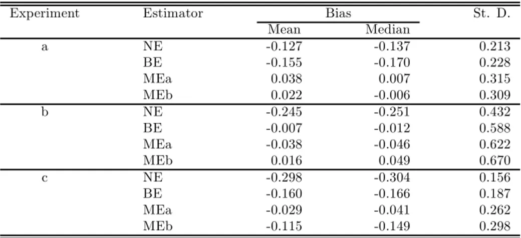
In this setting, CME is the only sampling problem that has to be taken into account in inference. In addition to the three estimators for RS previously considered in subsection 5.1.1 for the logit model, NE, MEa, and MEb, we also employ Buonaccorsi’s (1996) estimator for CME, denoted as BE. The estimation procedures for obtaining NE are the same as described in that subsection. Concerning the two MGMM estimators, MEa and MEb, now the nonparametric estimates of l_X1 are used directly in the moment indicators (59)-(61); see the directions for estimation with RS in subsection 3.4. Finally, BE was implemented by using the moment indicators (59) and (60) with l_X1 replaced by, respectively, 1 and _X1∗. Experiments were conducted in S-Plus, involving samples sizes of 300 and 1000 repetitions for each setting.

The statistics exhibited in Table 5, as well as the graphs in Figure 3, concerning estimates of θ1, show that the behaviour of the naive estimators is again unacceptable in terms of bias. As for the estimators accounting for measurement error, BE show a smaller variability across replications, probably due to not requiring the nonparametric estimation of l_X1. Comparing the results for the mean and median bias of the two estimators where σ is assumed known, BE and MEa, the former does better only in experiment b, showing larger mean and median biases in the other two cases, where the variance of the error-free covariate is larger. Moreover, BE has the disadvantage that in scheme a all statistics are slightly worse than those of NE, which creates serious doubts about its usefulness. Thus, in this example, the global behaviour of MEa is better, even with the larger σ of design c, which is encouraging, as we employ approximations based on small σ.

Table 5 about here Figure 3 about here

On the other hand, the results for MEb, which involve the estimation of σ, are also promising and very similar to those of MEa in designs a and b. However, its performance decays substantially in design c, due to the increase in σ. Even so, relative to NE, mean and median biases are reduced by more than 50% in all cases.

6

Conclusion

In this paper we have proposed a general framework to deal with the presence of CME in ES samples. First, a regression model to describe the observed data was specified by using Chesher’s (1991) asymptotic approximations for a small error variance. Then, we considered Imbens and Lan-caster’s (1996) efficient GMM estimators originally proposed for ES samples properly measured. After identifying the sources of bias of these estimators in the presence of CME, we suggested a modification to them in order to obtain approximately consistent estimators and outlined a score test sensitive to CME.

We found that the inconsistency of Imbens and Lancaster’s (1996) estimators when the co-variates’ contamination is not acknowledged, obtained by a Kiefer and Skoog-type (1984) measure adapted for the GMM framework, is a function of the approximate expectation of the moment indicators proposed by the former authors, taken with respect to the contaminated sampling joint distribution of the variable of interest, the error-prone covariates, and the stratum indicator. This approximation may be interpreted as the approximate bias induced by CME in the original mo-ment indicators. Using Chesher’s (2000) method, by subtracting this approximate bias function from the original moment indicators, we obtained modified moment indicators for which the ex-pectation taken under the approximate distribution of the observed data is approximately zero. Thus, we suggest the use of the traditional GMM techniques based on them to obtain approx-imately consistent estimators for the parameters of interest. A component of the approximate bias function is also employed in the efficient version of the score test to detect the presence of contamination.

All the major contributions of this paper require the calculation of the referred to approximate bias function. Though these calculations are often complicated, as they involve derivatives of the structural model and the nonparametric estimation of features of the error-free distribution of the covariates, once these functions are obtained, the score test for the presence of measurement error is easily implemented and, when the null hypothesis of absence of contamination is rejected, the employment of the MGMM estimators proposed here is straightforward.

The flexibility of this approach is especially visible in two levels. On the one hand, relative to the model specified for ES samples, it merely employs one additional mild assumption on the measurement error model, which requires that the measurement error is independently distributed from the latent covariates. On the other hand, neither the population marginal probability of each stratum nor the variance of the measurement error need to be known, although when this kind of information is available, it may be easily incorporated in the estimation procedure, allowing more efficient estimators to be obtained.