The dynamics between economic growth and living standards in EU Countries: A STATICO approach for the period 2006-2014

ES T U D I O S D E EC O N O M Í A AP L I C A D A VO L. 35-3 2017 PÁ G S. 629–652

The Dynamics between Economic Growth and

Living Standards in EU Countries: A

STATICO Approach for the Period 2006-2014

a _{Autonoma University of Lisbon, Rua de Santa Marta, n.º 47, 1150-293 Lisbon, Portugal. E-mail:} ajsantos@autonoma.pt, sribeiro@autonoma.pt

b

CIEO -Research Center for Spatial and Organizational Dynamics- University of Algarve, Campus de Gambelas-Building 9 - 8005-139, Faro, Portugal. E-mail: gcastela@ualg.pt,

info@ntavaresdasilva.com

ABSTRACT

The rate of economic growth is dissimilar between areas or regions, and these divergences generate potential impact on quality of life. The occurrence of the financial and economic crisis of 2008, can strengthen these gaps. Economic growth in this analysis includes six levels of gross domestic product growth rates (GDPgr) and seven variables with direct implications on the quality of life of families. The observations are fifteen EU countries, organized into three groups: northern, central and southern. The STATICO method (Simier et al., 1999) used in this research is a three-way multivariate analysis supported on a partial triadic analysis (PTA, Thioulose and Chessel, 1987) to find the stable part of the structure of a series of tables from 2006 to 2014, over a common structure resulting from the co-inertia analysis (Dolédec and Chessel, 1994) applied to each pair of an economic growth tables and a life standard tables. With this method, it was possible to extract the stable part of economic growth-life standard common relationships and to analyze the influences of the financial crisis of 2008

Keywords: Economic Growth, Life Standard, STATICO.

La dinámica entre el crecimiento económico y la calidad de

vida en los países de la UE: Un enfoque STATICO para el

período 2006-2014

RESUMEN

La tasa de crecimiento económico es diferente entre áreas o regiones, y estas divergencias generan un impacto potencial en la calidad de vida. La ocurrencia de la crisis financiera y económica de 2008, puede fortalecer estas brechas. El crecimiento económico en este análisis incluye seis niveles de tasas de crecimiento del producto interno bruto (PIBgr) y siete variables con implicaciones directas en la calidad de vida de las familias. Las observaciones son quince países de la UE, organizados en tres grupos: el norte, el centro y el sur. El método STATICO (Simier et al., 1999) utilizado en esta investigación es un análisis multivariante de tres vías apoyado en un análisis triádico parcial (PTA, Thioulose y Chessel, 1987) para encontrar la parte estable de la estructura de una serie de tablas del 2006 al 2014, sobre una estructura común resultante del análisis de co-inercia (Dolédec y Chessel, 1994) aplicado a cada par de tablas de crecimiento económico y tablas de calidad de vida. Con este método se pudo extraer la parte estable de las relaciones comunes de crecimiento económico-calidad de vida y analizar las influencias de la crisis financiera de 2008.

Palabras clave: Crecimiento económico, calidad de vida, STATICO.

JEL Classification: C0, E0 ____________

Artículo recibido en mayo de 2017 y aceptado en agosto de 2017

1. INTRODUCTION AND OBJECTIVES

Identifying the factors that evaluate the behavior of the economies, through the life standards of the populations, proves to be fundamental in the study of the economic dynamics. For historical and social reasons, the quality of life is also associated with the diversity observed in the levels of final consumption of the families and is distributed heterogeneously by economic spaces. Within the European Union (EU) this heterogeneity encompasses a space-time dimension that directly or indirectly influences the growth of economies, both in periods of stability and in periods of change. In this sense, the occurrence of crisis, as the financial, economic and sovereign debt crisis, can affect the performance of countries regarding economic growth and quality of life. In this context, a simultaneous analysis of economic growth and life standard data, which share, for the 2006-2014 period, encompassing three zones of the European economic space is pertinent. With the STATICO method (Simier et al., 1999; Thioulouse et al., 2004), it is possible to extract the stable part of the two data series common relationships and to analyze the influences of the financial crisis of 2008. This methodological approach can assess the structure of economic growth, in particular on stable and unstable consumer-based relationships in the EU, and help to investigate the effects of change in the economic dynamics. Investigating these dynamics and its distribution in EU, is, therefore, an essential step to understanding the differences in levels of economic growth, according to household consumption levels, which describe the quality of life in these regions.Therefore, the objectives of this study were to:

• Identify common structures between Economic Growth and Quality of Life descriptors;

• Identify the co-inertia and stability relations of the northern, central and southern countries and characterize the specificities of their behavioral evolution in the different phases of the crisis period;

• Evaluate the stability between the common structures of Economic Growth/Quality of Life relations for the period under analysis;

• To show STATICO as a useful methdology for the simultaneous analysis of economic growth and life standard data, which share, for the 2006-2014 period, the same sampling for the three zones of the European economic space.

This paper is structured in six chapters: 1) Introduction and Objective which contextualizes the research and its main goals, 2) Literature Review that synthetizes previous frameworks on heterogeneity of economic growth and life standards within EU countries and the occurrence of crisis, 3) Methodology which describes the methodological approach, the variables and observations, 4)

Results presents the main outputs and finally 5) Conclusions where the main findings are presented.

2. LITERATURE REVIEW

European countries continue to differ considerably from one another economically, not only in economic growth and development, in GDP growth rates and household consumption habits (EUROSTAT, 2017), but also to cultural identity is concerned (Kraus, 2003; Rosenberger, 2004).

According to Sepos (2016), historical, structural political and socio-economic problems in the peripheral countries further undermined their ability to cope with the institutional asymmetry of the European Monetary Union (EMU) and the global proliferation of financialization. On the other hand, the EU, with its politics, promoted increasing mobility, education of consumers, the proliferation of distance-spanning technologies and the pro-European media have contributed to the idea that distance has become irrelevant within Europe (Mahajan and Muller, 1994; Tellis et al., 2003; ter Hofstede, Steenkamp, and Wedel, 1999).

Nonetheless, the financial turmoil in 2007 and 2008, triggered by the collapse of the US subprime loan market (Shiller, 2008) followed by a global credit crunch and a banking crisis after Lehman Brothers bankruptcy had its toll on the European nations. This crisis swamped European banks and exposed significant shortcomings in EU financial market regulation and supervision (Quaglia et al., 2009). The EU member states agreed to set up measures to stabilize European banks in the short term, but credit shortages and a sharp contraction in world trade resulted in a severe recession.

Nevertheless, in the starting year of this study, the financialisation before the 2008 crisis created a new paradigm in the structure based on the asset prices and sovereign debt (Stockhammer et al., 2016) in 2009, visible since 2010.

By the beginning of 2010, budget deficits in Greece, Portugal, Ireland, and Spain were close to or above 10 percent (Wallace et al., 2015). The global financial crisis paved the way for a euro area sovereign debt crisis as financial markets lost confidence in the ability of governments in these countries to honor their national debts. It became evident that euro area member states would require financial assistance to surpass this cycle. This financial assistance, by way of loans were co-financed by EU member states and the International Monetary Fund (IMF) with the disbursal of loan instalments contingent on compliance with an economic adjustment programme overseen by officials from the ‘troika’ of the Commission, the ECB, and the IMF encompassing both member states that had not adopted the single currency and Eurozone members. No member state was immune from this sudden slowdown, but those that entered the financial crisis with serious macroeconomic imbalances were, the most hit. No member state

that sought external financial assistance during the sovereign debt crisis escaped the harsh effects of imposed austerity (Wallace et al., 2015). The financial and sovereign debt crisis subjected European nations to different levels hardship, suffering and misery, and contributed to the growing divide and inequality between the EU nations from the centre and periphery (Sepos, 2016).

3. METHODOLOGY

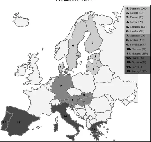
The study was conducted in fifteen EU countries, belonging to 3 areas of the northern, central and southern, using annual data for the period 2006-2014 (Figure 1).

Figure 1

15 countries of the EU

3.2. Variables

The GDP growth rate as a measure of economic growth/development is widely used to measure the economic performance of a country between periods. The evolution of GDP growth supports the evaluation of economic policies and determines if an economy is in recession. Economic growth is the increase in the market value of the goods and services produced by an economy, conventionally per year. It is usually measured as the percent rate of growth in real GDP. An increase in growth can be caused by the more efficient use of inputs or by increases in inputs such as capital, population, and even territory. Regarding the GDP components and related indicators of economic output, imports and exports, domestic private and public consumption and investments, as well as data on the distribution of income and savings can give valuable insights into the driving forces in an economy and thus be the basis for the design, monitoring and evaluation of specific EU policies (EUROSTAT, 2017). In previous work, it has been shown that there are differences in economic growth across European regions can be reasonably well explained by an approach that focuses on innovation activities in the region, the potential for exploiting technologies developed elsewhere and complementary factors affecting the exploitation of this potential (Fagerberg and Verspagen, 1996; Fagerberg et al., 1997; Cappelen et al., 1999). There are other enhancing (or growth-retarding) factors at the regional level. Household consumption habits vary substantially among the EU Member States (EUROSTAT, 2017). Factors such as culture, income, weather, household composition, economic structure and degree of urbanisation can all have an impact on habits in each country. National accounts data also reveal that a little over a fifth of total household consumption expenditure is devoted to housing, water, electricity, gas and other housing fuels (EUROSTAT, 2017b). Expenditure on transport and food and non-alcoholic beverages constitute the next two most important categories in the EU, at about the same level and together accounting for a little more than a quarter of total household consumption expenditure. The household expenditure is possible proxy to measure life standards as “consumption is a key indicator of citizens’ wellbeing, with housing, energy, transport and food accounting for about half of total household expenditure” (EUROSTAT, 2017b). “The population consumption expenditures were taken into consideration, because they measure the objective economic dimension of the standard of living” (Florea et al., 2016).

To analyze the spatiotemporal variability in the co-structure formed by economic growth and life standards, it was considered, for the period between 2006 and 2014 (Table 1): a) 6 Levels of real GDP growth rates; and b) 7 Types of household expenditure on essential goods and services.

Table 1

Economic growth and life standards descriptors

200 6 -20 14 E CO NO M IC GR OW T H

GDP growth rate between -15% and -10% EG1

GDP growth rate between -10% and -5% EG2

GDP growth rate between -5% and 0% EG3

GDP growth rate between 0% and 5% EG4

GDP growth rate between 5% and 10% EG5

GDP growth rate between 10% and 15% EG6

L IF E S T AN DARDS

Household expenditure with Food and non-Alcoholic Beverages LS1 Household expenditure with Clothing and Footwear LS2 Household expenditure with Housing, Water, Electricity, Gas and other Fuels LS3

Household expenditure with Transport LS4

Household expenditure with Leisure, Recreation and Culture LS5

Household expenditure with Education LS6

Household expenditure with Restaurants and Hotels LS7

Source: Own elaboration.

3.3. Design

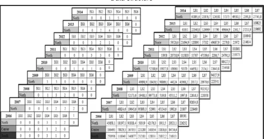
STATICO was used for the simultaneous analysis of two series of data, which share, for the 2006-2014 period, the same sampling for the three zones of the European economic space. The first series, descriptive of economic growth, is composed of nine parameterized matrices with 6 levels of real GDP growth rates, accounting for the occurrence of each level by aggregates of countries from the north (6 countries), the center (5 countries) and south (4 countries) of the EU. The second series consists of 9 matrices with 7 parameters describing life standards (Figure 2).

Figure 2

Data structure

3.4. The STATICO

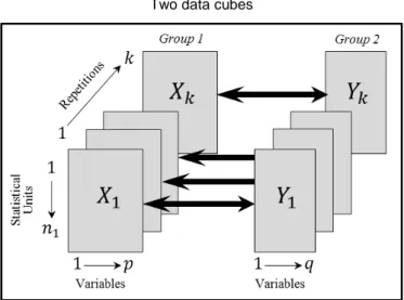
The STATICO method (Simier et al., 1999; Thioulouse et al., 2004) is used to analyze two data cubes (Figure 3), to evaluate a common structure between pairs of tables (one of each data cube) and the stability of that structure, during the sampling period. The STATICO is executed in three steps: (1) the first step consists in analyzing each table by a basic method, traditionally a PCA, properly normalized or centered; (2) then each pair of tables is linked by a co-inertia analysis (Dolédec and Chessel, 1994) which provides a mean image of the existing co-structure; (3) Finally, a Partial Triadic Analysis (Thioulouse and Chessel, 1987) is used to analyze this sequence.

Figure 3

Two data cubes

Source: Adapted from Simier et al. (1999).

In order to better understand the STATICO, consider a 𝐾𝐾 study consisting of a 𝑋𝑋𝑘𝑘 matrix with 𝑝𝑝 variables for the first group described by 𝑛𝑛𝑘𝑘 statistical units, and

a 𝑌𝑌_𝑘𝑘 matrix with 𝑞𝑞 variables, for the second group with the same statistical units. This double study is repeated 𝐾𝐾 times and, from one repetition to another, the list of variables is constant, while the list of the statistical units may vary.

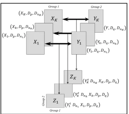
If we consider 𝑋𝑋𝑡𝑡(𝑋𝑋₁𝑡𝑡, … , 𝑋𝑋_𝐾𝐾𝑡𝑡) and 𝑌𝑌𝑡𝑡(𝑌𝑌₁𝑡𝑡, … , 𝑌𝑌_𝐾𝐾𝑡𝑡), for a complete sampling of all statistical units, for all repetitions one obtains a pair of data cubes. Each of these matrices is part of a duality diagram (Escoufier, 1987), respectively �𝑋𝑋𝑘𝑘, 𝐷𝐷𝑝𝑝, 𝐷𝐷𝑛𝑛𝑘𝑘� and �𝑌𝑌𝑘𝑘, 𝐷𝐷𝑞𝑞, 𝐷𝐷𝑛𝑛𝑘𝑘� (Figure 4).

The diagonal metrics 𝐷𝐷_𝑝𝑝 and 𝐷𝐷_𝑞𝑞 are fixed and independent of repetition. The metric of the unit’s weights 𝐷𝐷_{𝑛𝑛𝑘𝑘} is common to both schemes, allowing a

co-inertia analysis of the two matrices. Thus, the 𝐾𝐾 co-inertia schemes share both the same dimension of the matrices and the same metric. In the 𝑘𝑘 repetition, the 𝑋𝑋_𝑘𝑘 matrix, inserted into the �𝑋𝑋_𝑘𝑘, 𝐷𝐷_𝑝𝑝, 𝐷𝐷_{𝑛𝑛𝑘𝑘}� schema, and the 𝑌𝑌_𝑘𝑘matrix inserted into the �𝑌𝑌𝑘𝑘, 𝐷𝐷𝑞𝑞, 𝐷𝐷𝑛𝑛𝑘𝑘� scheme gave rise to the co-inertia scheme �𝑌𝑌𝑘𝑘𝑡𝑡 𝐷𝐷𝑛𝑛𝑘𝑘 𝑋𝑋𝑘𝑘, 𝐷𝐷𝑝𝑝, 𝐷𝐷𝑞𝑞�,

commonly denoted by 𝑍𝑍 = 𝑌𝑌_𝑘𝑘𝑡𝑡 𝐷𝐷_{𝑛𝑛𝑘𝑘} 𝑋𝑋_𝑘𝑘.

According to the definition of the Partial Triadic Analysis (PTA), finding a co-inertia compromise requires re-focusing on the 𝛼𝛼_𝑘𝑘values, such that �∑𝐾𝐾𝑘𝑘=1𝛼𝛼𝑘𝑘 𝑍𝑍𝑘𝑘, 𝐷𝐷𝑝𝑝, 𝐷𝐷𝑞𝑞� has a maximum inertia, under the constraint ∑𝐾𝐾𝑘𝑘=1𝛼𝛼𝑘𝑘2= 1.

Figure 4

STATICO layout

Source: Adapted from Simier et al. (1999).

In practice, the compromise of PTA is a fictitious co-inertia analysis in which the cross-table, 𝑍𝑍 = 𝑌𝑌_𝑘𝑘𝑡𝑡 𝐷𝐷_{𝑛𝑛𝑘𝑘} 𝑋𝑋_𝑘𝑘, represents a weighted average of the 𝐾𝐾 cross-tables. Its columns are 𝑋𝑋 columns and their rows are 𝑌𝑌 columns. Their analysis provides their own values, a column ordering (hence the 𝑝𝑝 variables of 𝑋𝑋), and a row ordering (hence the 𝑞𝑞 variables of 𝑌𝑌) . Any PTA can be projected on the basis of supplementary points, the elements of the 𝐾𝐾 separate analyzes of co-inertia on the axes, and the components of the compromise: columns, the axes and the principal components of 𝑍𝑍_𝑘𝑘(1 ≤ 𝑘𝑘 ≤ 𝐾𝐾).

Due to co-inertia, a new dimension is involved here: that of statistical units. In fact, all lines of 𝑋𝑋 (statistical units) and the components of the commitment, all lines of 𝑌𝑌 (also statistical units), can be preserved in additional lines on the axes of inertia of the commitment. In general, to normalize their coordinates to retain in the co-inertia the part of the "correlation", the projections of the statistical units, respectively, of the spaces and lines of the 𝐾𝐾 matrices of 𝑋𝑋 and 𝑌𝑌 can be combined. The representation of this double dispersion of multiple points, per table, allows to judge on the evolution of all the tables in the implementation of the common co-structure. It is also possible to standardize, by table, the coordinates of the supplementary lines to express the instantaneous correlation.

4. RESULTS

The method was performed in three phases: (1) the first consisted of analysing each data matrix through a standard PCA of the life standards descriptors and a centralized PCA of the economic growth descriptors; (2) - then, per year, each pair of matrices was linked by a co-inertia analysis which provided a mean image of the existing co-structure (cross-covariance table); (3) - finally, a PTA was used to analyse the sequence of co-structures using a three-step procedure: a) - analysis of the interstructure; B) - analysis of the compromise and, c) - analysis of the intra-structure (or trajectories).

In this way, it was possible not only to understand the economic dynamics of the EU, but also to discuss the relationship between levels of economic growth and patterns of consumption. Since the descriptor structures under analysis are often inter-correlated, complex behavioural patterns were found that are not possible to directly analyse from the original sources. And while there are a variety of multivariate techniques that can potentially address this problem, tools that take into account the temporal variation of the descriptor parameters and the influence of one over the other are rare.

The present contribution proved to be particularly suitable to detect that matrices, among several, constitute a common typological basis, which is not directly visible in the particularities of each data matrix, and which group, between two, of descriptors constitutes a common typology of objects described in each of the matrices. In this way, it was possible to study the stability of the relationship between economic growth and life standards, when both vary over time, on the influence of the analogies detected in consumption patterns. Both the calculations and the graphs presented in this work were performed using the ADE-4 software of the R program (Thioulouse et al., 1997) which is available at http://pbil.univ-lyon1.fr/ADE-4.

As already mentioned above, the STATICO method is a PTA on the sequence of cross product tables, so the compromise is also a cross product

table, with the 6 types of economic growth rates in rows and 7 types of household expenditure on essential goods and services in columns. The euro zones have disappeared from this table, but they can be projected as supplementary elements to help interpret the results of the analysis.

4.1. The interstructure

It was observed from the RV matrix (vectorial correlations of Escoufier (1987)) that the inter-matrix correlations are not all positive, which means that there is an inversion in the structure of one sample for another sample and that the distribution patterns of co-inertia by the euro-zones were not common to all sampling years.

Through Figure 5 and for the time horizon under analysis, 3 distinct realities in the interstructure are visible: a post-crisis period (2010, 2011, 2012, 2013 and 2014) signalled in black, under the axis of greater inertia, and a pre-crisis period (2006, 2007, 2008 and 2009), marked in red under the axis of lower inertia.

Figure 5

Interstructure

Source: Adapted from ADE4 outputs.

The pre-crisis period, for the years 2006, 2007 and 2008, reflects a lower inertia and weight. The "turnaround" year (2009) also shows a reduced inertia, although with a greater weight, and is uncorrelated or negatively correlated either with the pre-crisis years or with the post-crisis years. The post-crisis period (2010, 2011, 2012, 2013 and 2014) presents each year with positive and high correlations between them.

a) Greater inertia for the post-crisis period, with years with very similar norms and very positively correlated. This situation reveals, on average, a high stability in the data structure, which makes it possible to assess in an identical way the way in which these years reflected a common co-structure between economic growth and quality of life;

b) Less inertia for the pre-crisis period, with years with very different norms and little correlation between them. This situation reveals, on average, an instability in the data structure, which makes it difficult to assess identically how these years have manifested a common co-structure between economic growth and quality of life.

4.2. The compromise

The analysis of the compromise on the descriptors of growth (Figure 6) generally shows, on the axis of greatest inertia, an increase, on average, in growth rates, from left to right. Nevertheless, it is observed that the EG1, EG2 and EG6 growth rates, with lower variability, showed a negative correlation with the first axis, contrary to the higher variability rates EG3, EG4 and EG5, which presented positive correlations.

Figure 6

Compromise for the descriptors of economic growth

Source: Adapted from ADE4 outputs.

Similarly, for the consumption descriptors of life standards (Figure 7), on the axis of greatest inertia, there is a rise in the same direction (from left to right), which increases from household expenses with Restaurants and Hotels to expenses with Leisure, Recreation and Culture. All these expenses present high variability and are positively correlated with the first axis.

Figure 7

Compromise for the descriptors of life standards

Source: Adapted from ADE4 outputs.

In summary, Figures 6 and 7 describe, on average, for the period 2006-2014: a) A relationship between growth rates ranging from -5% to 10% (1st and

4th quadrants) with the increase of household expenses in all types of goods and services. This typology (TYPOLOGY 1) makes it possible to evaluate the temporal variation of the common co-structure between economic growth and life standards and the influence of one over the other;

b) A relation between the lowest growth rates (from -15% to -5% in the 2nd and 3rd quadrants) and the reduction of household expenditures on all types of goods and services. This typology (TYPOLOGY 2) also makes it possible to evaluate the temporal variation of the common co-structure between economic growth and life standards and the influence of one over the other;

The two typologies detected, which are not directly visible in the original data, allow us to study the common co-structure between economic growth and life standards, when both vary over time, either in periods of stability (post-crisis) or in periods of instability (pre-(post-crisis) and on the influence of consumption patterns.

4.3. The intrastructure

This phase of the PTA also consists in analysing the existing correlations between the descriptors of each original data matrix in the compromise space.

By projecting them as supplementary elements, it is possible to study the evolution of trajectories throughout the study period.

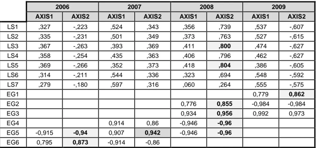
Table 2 points out, for the pre-crisis period, the highest correlations of the life standards and economic growth descriptors with the secondary axis of the compromise, which is the axis associated to the instable years of 2006, 2007, 2008 and 2009 in the interstructure.

Table 2

Correlations of the original variables with the axis of the compromise space for the pre-crisis period

2006 2007 2008 2009

AXIS1 AXIS2 AXIS1 AXIS2 AXIS1 AXIS2 AXIS1 AXIS2

LS1 ,327 -,223 ,524 ,343 ,356 ,739 ,537 -,607 LS2 ,335 -,231 ,501 ,349 ,373 ,763 ,527 -,615 LS3 ,367 -,263 ,393 ,369 ,411 ,800 ,474 -,627 LS4 ,358 -,254 ,435 ,363 ,406 ,796 ,462 -,627 LS5 ,369 -,266 ,352 ,373 ,418 ,804 ,386 -,605 LS6 ,314 -,211 ,544 ,336 ,323 ,694 ,548 -,592 LS7 ,279 -,180 ,597 ,316 ,060 ,264 ,555 -,575 EG1 0,779 0,862 EG2 0,776 0,855 -0,984 -0,984 EG3 0,934 0,956 0,992 0,973 EG4 0,914 0,86 -0,946 -0,96 EG5 -0,915 -0,94 0,907 0,942 -0,946 -0,96 EG6 0,795 0,873 -0,914 -0,86

Source: Adapted from ADE4 outputs.

Figure 8 shows the projections in the compromise space of the most relevant correlations of the original variables for the pre-crisis period.

Figure 8

Projections of the most relevant correlations of the original variables for the pre-crisis period

Figure 8 (Continue)

Projections of the most relevant correlations of the original variables for the pre-crisis period

2008 2009

Source: Adapted from ADE4 outputs.

Of note is the year 2008, where growth rates vary from -10% to 0%, associated with an increase in household expenditures with Housing, Water, Electricity, Gas and other Fuels and with Leisure, Recreation and Culture.

The Table 3 highlights in grey, for the post-crisis period, the highest correlations of the life standards and economic growth descriptors with the principal axis of the compromise, which is the axis associated to the stable years of 2010, 2011, 2012, 2013 and 2014 in the interstructure.

Table 3

Correlations of the original variables with the axis of the compromise space for the post-crisis period

2010 2011 2012 2013 2014

AXIS1 AXIS2 AXIS1 AXIS2 AXIS1 AXIS2 AXIS1 AXIS2 AXIS1 AXIS2

LS1 -0,887 ,214 -,696 ,288 -0,939 -,341 -,549 -0,831 -,763 -,552 LS2 -0,87 ,263 -,652 ,332 -0,933 -,085 -,595 -,797 -,802 -,379 LS3 -,790 ,415 -,588 ,388 -0,874 ,120 -,624 -,772 -,806 -,272 LS4 -,785 ,421 -,548 ,419 -,654 ,474 -,703 -,676 -,769 -,012 LS5 -,629 ,587 -,484 ,464 -,177 0,821 -,684 ,218 -,397 ,616 LS6 -0,898 ,172 -,717 ,265 -0,93 -,397 -,538 -0,838 -,742 -,603 LS7 -0,909 ,113 -,758 ,216 -0,905 -,485 -,521 -0,848 -,717 -,652 EG1 EG2 0,99 0,978 0,996 0,989 0,997 0,993 EG3 0,789 0,87 0,755 0,846 0,975 0,998 0,993 0,998 0,974 0,998 EG4 -0,99 -0,978 -0,996 -0,989 -0,993 -0,998 -0,997 -0,992 -0,996 -0,991 EG5 -0,99 -0,978 0,756 0,847 ,628 ,743 EG6

Figure 9 shows the projections in the commitment space of the most relevant correlations of the original variables for the post-crisis period.

Figure 9

Projections of the most relevant correlations of the original variables for the post-crisis period

2010 2011

2012 2013

2014

Source: Adapted from ADE4 outputs.

The years 2010 and 2014 stand out. 2010 shows a decrease in the expenses of families with Food and Non-Alcoholic Beverages, Clothing and Footwear,

Education and Restaurants and Hotels associated with economic growth rates ranging from 0% to 10%. And, 2014 shows a decrease in the expenses of households with Clothing and Footwear and Housing, Water, Electricity, Gas and other Fuels associated with economic growth rates varying between 0% and 5%.

The reproduction of the trajectories in the Euclidean image of the compromise is based on the representation in this image of the clouds of the economic growth and life standards descriptors. In this context, the trajectory of each descriptor will be represented in the plan that includes the dimension with greater inertia. In this way it's possible point out the years in which a consistent structure is revealed. Thus the evolution of the common co-structure between economic growth and life standards, when both vary over time, either in periods of stability (post-crisis) or in periods of instability (pre-crisis) is therefore observed.

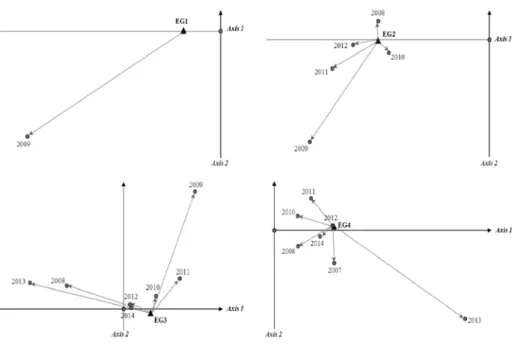
Figure 10 describes, through the distances to the average, the evolution of economic growth rates observed during the period between 2006 and 2014.

Figure 10

Figure 10 (Continue)

Distances to the average for the six descriptors of economic growth

Source: Adapted from ADE4 outputs.

2007 was the year that most contributed to the highest rate of economic growth (EG6, from 10% to 15%). 2009 was the year that most contributed to the stability of three economic growth rates (EG1, EG2 and EG3). That is, it was the most relevant year in the stability of negative economic growth rates (from -15% to 0%). 2011 was the year that most contributed to the second highest rates of economic growth (EG5, from 0% to 10%). 2013 was the year that most contributed to economic growth rates ranging from 0% to 5% (EG4).

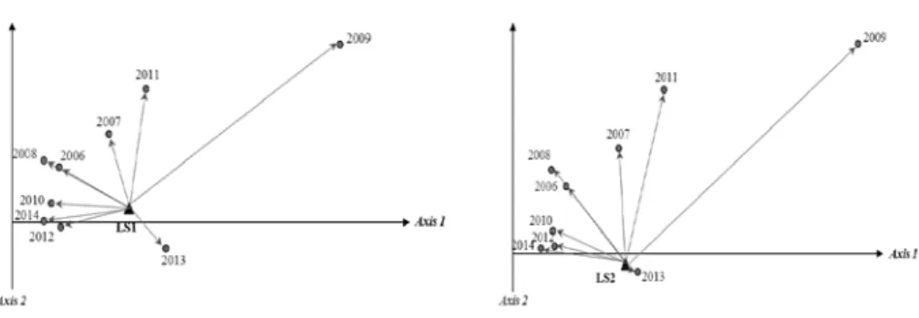
Figure 11 describes, through the distances to the average, the evolution of life standards indicators observed during the period between 2006 and 2014.

2009 was also the year that most contributed to the stability of all life standards indicators observed during the period between 2006 and 2014. That is, it was the most relevant year in the stability of household expenses in all types of goods and services.

Figure 11

Figure 11 (Continue)

Distances to the average for the seven descriptors of life standards

Source: Adapted from ADE4 outputs.

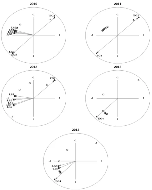
Lastly, Figure 12 describes, through the trajectories, the evolution of economic growth rates and the life standards indicators observed during the period between 2006 and 2014.

In the countries of the northern zone of the EU, and regarding economic growth, it is clear that there is a wider trajectory during the pre-crisis period, which is associated with greater variability, within the lowest growth rates, creating some instability. Starting from 2009, and during the post-crisis period, with higher growth rates, is visible a tighter evolutionary path (less variability) which is compatible with stability on economic growth.

Figure 12

Trajectories for the economic growth and for the life standards

EU North

EU Central

EU South

Source: Adapted from ADE4 outputs.

On the other hand, about the trajectories of living standards indicators, there is some cohesion in the evolution of household expenditure. However, in 2009 there was a small reduction in household expenses, from which there were small and homogenous increases in all types of expenditure on essential goods and services.

In the countries of the central zone of the EU, and regarding economic growth, it is observed a tighter trajectory over almost the whole period under review, except the year 2009 which showed a clear reversal of the GDP rates.

During the pre-crisis period, there were higher growth rates, which declined sharply in 2009, to stabilize again in the post-crisis period, at similar levels to those in the pre-crisis period. However, it can be said that there was a tighter evolutionary path of GDP rates in the post-crisis period (less variability) which is compatible with stability on economic growth. The pre-crisis period, because of 2009, is associated with greater variability, within the higher growth rates, creating in this way some instability on economic growth.

On the other hand, about the trajectories of living standards indicators, there is also some cohesion in the evolution of household expenditure. However, in 2009 there was a small reduction in household expenses, from which there were substantial increases in all types of expenditure on essential goods and services, until 2014.

Lastly, in the countries of the southern zone of the EU with regard to economic growth, it is also observed a tighter trajectory over the whole period under review. However, higher rates of economic growth are observed in the pre-crisis period, which visibly decreases from 2009 until 2012 to grow back up to 2014. This means that there was greater variability in terms of GDP rates and, therefore, less stability on economic growth.

About the trajectories of living standards indicators, from 2009 there is no cohesion in the evolution of household expenditure. While up to 2009 were observed substantial increases in all types of expenditure on essential goods and services, in the post-crisis reductions were visible.

5. CONCLUSION

I. The pre-crisis period reveals, on average, instability in the data structure, which makes it difficult to assess a common co-structure between economic growth and living standards. The post-crisis period reveals, on average, high stability in the data structure, which makes it possible to assess a common co-structure between economic growth and living standards.

II. Two typologies were detected: a) - Growth rates ranging from -5% to 10% are associated with the increase of household expenses; b) - Growth rates from -15% to -5% are associated with the reduction of household expenditures.

III. For the pre-crisis period, the highest correlations of the life standards and economic growth descriptors highlight 2008, where growth rates vary from -10% to 0%, associated with an increase in expenditures with Housing, Water, Electricity, Gas and other Fuels and with Leisure, Recreation and Culture. For the post-crisis period, the years 2010 and 2014 stand out. 2010 shows a decrease in expenditures with Food and

Non-Alcoholic Beverages, Clothing and Footwear, Education and Restaurants and Hotels associated with economic growth rates ranging from 0% to 10%. And, 2014 shows a decrease in expenditures with Clothing and Footwear and Housing, Water, Electricity, Gas and other Fuels associated with economic growth rates varying between 0% and 5%.

IV. 2007 was the year that most contributed to the highest rate of economic growth (from 10% to 15%). 2009 was the year that most contributed to the stability of three economic growth rates (from 15% to 10%; from -10% to -5%; from -5% to 0%). 2011 was the year that most contributed to the second highest rates of economic growth (from 0% to 10%). 2013 was the year that most contributed to economic growth rates ranging from 0% to 5%.

V. 2009 was also the year that most contributed to the stability of all life standards indicators observed during all the period in analysis. That is, it was the most relevant year in the stability of household expenditures. VI. In the countries of the northern zone of the EU and regarding economic

growth, it is clear that is observed a wider trajectory during the pre-crisis period, which is associated with greater variability, within the lowest growth rates, creating some instability. From 2009, and during the post-crisis period, with higher growth rates, is visible a tighter evolutionary path which is compatible with stability. About the trajectories of living standards indicators, there is some cohesion in the evolution of household expenditure. However, in 2009 there was a small reduction in household expenses, from which there were small and homogenous increases in all types of expenditure.

VII. In the countries of the central zone of the EU, and in terms of economic growth, it is observed a tighter trajectory over almost the whole period under review, except the year 2009 which showed a clear reversal of the GDP rates. During the pre-crisis period there were higher growth rates, which declined sharply in 2009, to stabilize again in the post-crisis period, at similar levels to those in the pre-crisis period. However, it can be said that there existed a tighter evolutionary path of GDP rates in the post-crisis period which is compatible with stability. The pre-crisis period, because of 2009, is associated with greater variability, within the higher growth rates, creating some instability. With regard to the trajectories of living standards indicators, there is also some cohesion in the evolution of household expenditure. However, in 2009 there was a small reduction in household expenses, from which there were substantial increases in all types of expenditure until 2014.

VIII. Lastly, in the countries of the southern zone of the EU about economic growth, it is also observed a tighter trajectory over the whole period under review. However, higher rates of economic growth are observed in the pre-crisis period, which visibly decreases from 2009 until 2012 to grow back up to 2014. This means that there was greater variability regarding GDP rates and, therefore, less stability on economic growth. About the trajectories of living standards indicators, from 2009 there is no cohesion in the evolution of household expenditure. Up to 2009 were observed substantial increases in all types of expenditure and in the post-crisis were visible reductions.

IX. This STATICO approach provided a diagnosis to the academia and policy makers encompassing a behavioural characterization of three zones of the European economic space, which highlights particular responses of each zone to different macroeconomic contexts, namely expansionary versus contractionary policies, and therefore points to the need for specific instead of generalist EU strategies.

BIBLIOGRAPHY REFERENCES

CAPPELEN, A., FAGERBERG, J. and VERSPAGEN, B. (1999). “Lack of Regional Convergence”. In Fagerberg, J., Guerrieri, P. and Verspagen, B. (eds): The Economic

Challenge for Europe. Adapting to Innovation Based Growth (Aldershot: Edward Elgar).

DOLÉDEC, S. and CHESSEL, D. (1994). “Co-inertia analysis: an alternative method for studying species-environment relationships”. Freshwater Biology, 31, pp. 277-294.

ESCOUFIER, Y. (1987). The duality diagram: a means for better practical applications. In Develoments in Numerical Ecology. (pp. 139-156). Springer Berlin Heidelberg. EUROSTAT (2017). GDP and household accounts at regional level. Available from:

http://ec.europa.eu/eurostat/statistics-explained/index.php [Accessed: 11 /05/2017]. EUROSTAT (2017b). Household consumption expenditure - background. Available from:

http://ec.europa.eu/eurostat/statistics-explained/index.php/Household_ consumption_expenditure_-_background [Accessed: 11 /05/2017].

FAGERBERG, J. and VERSPAGEN, B. (1996). ‘Heading for Divergence? Regional Growth in Europe Reconsidered’. Journal of Common Market Studies, Vol. 34, No. 3, pp. 431-48. Fagerberg, J.,

FLOREA, N. M., MEGHISAN, G. M., and NISTOR, C. (2016). “Multiple Linear Regression Equation for Economic Dimension of Standard of Living”. Finante-provocarile viitorului

(Finance-Challenges of the Future), 1(18), pp. 103-108.

GERSTBERGER, C., and YANEVA, D. (2013). “Analysis of EU-27 household final consumption expenditure-Baltic countries and Greece still suffering most from the economic and financial crisis”. Eurostat Statistics in focus ,2/2013, p. 1.

KRAUS, P.A. (2003). “Cultural pluralism and European policy-building”. Journal of

MAGONE, J. M., LAFFAN, B., and SCHWEIGER, C. (Eds.). (2016). Core-Periphery

Relations in the European Union: power and conflict in a dualist political economy.

Routledge.

MAHAJAN, V., and MULLER, E. (1994). “Innovation diffusion in a borderless global market: Will the 1992 unification of the European Community accelerate diffusion of new ideas, products, and technologies?”. Technological forecasting and Social

Change, 45(3), pp. 221-235.

QUAGLIA, L., EASTWOOD, R., and HOLMES, P. (2009). “The Financial Turmoil and EU

Policy Co‐operation in 2008”. JCMS: Journal of Common Market Studies, 47(s1), pp.

63-87.

ROSENBERGER, S. (2004). “The other side of the coin”. Harvard International Review, 26(1), pp. 22-25.

SEPOS, A. (2016). “The centre-periphery divide in the Eurocrisis”. Core-periphery

Relations in the European Union: Power and Conflict in a Dualist Political Economy,

35.

SHILLER, R., and QUINN, B. (2008). “The Subprime Solution: How Today's Financial Crisis Happened, and What To Do About it”. Financial Regulator, 13(2), pp. 75.

SIMIER, M., BLANC L., PELLEGRIN F., and NANDRIS D. (1999). “Approche simultanée de K couples de tableaux : Application a l'étude des relations pathologie végétale- environnement”. Revue de Statistique Appliquée, 47, pp. 31-46.

STEENKAMP, J.-B.E.M., TER HOFSTEDE, F., and WEDEL, M. (1999). “A cross-national investigation into the individual and national cultural antecedents of consumer innovativeness”. Journal of Marketing, 63 (2), pp. 55-69.

STOCKHAMMER, E., and WILDAUER, R. (2016). “Debt-driven growth? Wealth, distribution and demand in OECD countries”. Cambridge Journal of Economics, 40(6), pp. 1609-1634.

TELLIS, G.J., STREMERSCH, S., and YIN, E. (2003). “The international takeoff of new products: The role of Economics, culture, and country innovativeness”. Marketing

Science, 22(2), pp. 188-208.

THIOULOUSE, J., and D. CHESSEL (1987). “Les analyses multi-tableaux en écologie factorielle. I De la typologie d’état à la typologie de fonctionnement par l’analyse triadique”. Acta Oecologica, Oe-cologia Generalis, 8, pp. 463-480.

THIOULOUSE, J., CHESSEL, D., DOLÉDEC, S., and OLIVIER, J. M. (1997). “ADE-4: a multivariate analysis and graphical display software”. Statistics and computing, 7(1), pp. 75-83.

THIOULOUSE, J., SIMIER, M., and CHESSEL, D. (2004). “Simultaneous analysis of a sequence of paired ecological tables”. Ecology, 85(1), pp. 272-283.

VERSPAGEN, B. and CANIËLS, M. (1997). “Technology, Growth and Unemployment across European Regions”. Regional Studies, Vol. 31, No. 5, pp. 457-66.

WALLACE, H., POLLACK, M. A., and YOUNG, A. R. (Eds.). (2015). Policy-making in the

SOFTWARE:

ADE4 Package for r-program

Dray, S. and Dufour, A.B. (2007): The ade4 package: implementing the duality diagram for ecologists. Journal of Statistical Software, 22(4), pp. 1-20.

R-program

R Development Core Team (2008). R: A language and environment for statistical computing. R Foundation for Statistical Computing, Vienna, Austria. ISBN 3-900051-07-0, URL http://www.R-project.org.