Processamento automático de uma rede GPS permanente

P

ROCESSAMENTO

A

UTOMÁTICO DE

UMA

R

EDE

G

PS

P

ERMANENTE

Gonçalo Prates

Licenciado em Engenharia Geográfica

Dissertação submetida para a obtenção do grau de

Mestre em Ciências e Engenharia da Terra

P

ROCESSAMENTO

A

UTOMÁTICO DE

UMA

R

EDE

G

PS

P

ERMANENTE

Gonçalo Prates

Licenciado em Engenharia Geográfica

Orientador: Prof. Doutor Virgílio Mendes

Dissertação submetida para a obtenção do grau de

Mestre em Ciências e Engenharia da Terra

A

UTOMATED

P

ROCESSING OF A

P

ERMANENT

G

PS

N

ETWORK

Gonçalo Prates

Diploma in Engenharia Geográfica

Supervisor: Prof. Doctor Virgílio Mendes

Dissertation submitted in partial fulfillment of the

requirements for the degree of Master of Sciences

in Ciências e Engenharia da Terra

September 2003

Sumário

O principal objectivo do Sistema de Posicionamento Global (GPS) é providenciar navegação e tempo precisos, em qualquer local do globo e sob quaisquer condições atmosféricas, 24 horas por dia. Para além disso, com base no grande número de estações permanentes, os estudos da atmosfera, do campo gravitacional e das modificações da crosta terrestre surgem como algumas das mais interessantes aplicações do GPS.

Estas aplicações são apoiadas em redes de estações GPS, como as redes IGS (International GPS

Service) e EPN (European Reference Frame (EUREF) Permanent Network), que facultam as suas

bases de dados de observações GPS, contribuindo indirectamente para o aumento de redes regionais a nível global. O IGS providencia também órbitas precisas dos satélites GPS, mapas de conteúdo total de electrões na ionosfera e modelos cinemáticos globais para a tectónica. Nos últimos anos, várias estações GPS permanentes foram também instaladas em Portugal, originando grandes bases de dados de observações GPS. São vários os produtos que podem ser potencialmente obtidos usando estas observações GPS, existindo no entanto necessidade de implementar sistemas automáticos que facilitem as morosas operações de processamento de observações GPS.

O principal objectivo deste estudo é implementar um sistema automático de processamento, com base no Bernese GPS Software 4.2, mais especificamente no Bernese Processing Engine, para

processar as observações GPS recolhidas por uma rede de estações permanentes localizadas na região do Atlântico Nordeste, e que inclui estações mantidas pela Faculdade de Ciências da Universidade de Lisboa (FCUL).

A rede é constituída por estações IGS (Madrid, Maspalomas, Ponta Delgada, San Fernando e Villa Franca del Campo), estações EUREF (Cascais, Vila Nova de Gaia e Lagos) e estações da FCUL (Flores, Graciosa, Santa Maria, Instituto de Meteorologia da Madeira, Observatório Astronómico de Lisboa Norte e Observatório Astronómico de Lisboa Sul). Esta rede abrange a Península Ibérica e os Arquipélagos dos Açores, Madeira e Canárias, o que possibilita uma análise geodinâmica da região, onde interagem três placas tectónicas.

O Bernese GPS Software 4.2, desenvolvido na Universidade de Berna, assenta em programas Fortran controlados por shell scripts. As opções de processamento são introduzidas através de

painéis que podem ser preenchidos com o auxílio do sistema de menus do software.

por um conjunto de shell scripts incluídas no Bernese GPS Software 4.2, para além de algumas

variáveis e parâmetros associados às operações definidas.

A construção do PCF é extremamente útil no preenchimento de todos os painéis necessários aos programas requeridos pelas operações de processamento listadas. Deste modo, os vários painéis foram facilmente preenchidos utilizando o Panel Editing Tool incluído no sistema de menus do Bernese GPS Software específico para o Bernese Processing Engine.

O software de processamento necessita ainda que alguma informação respeitante às estações seja definida a priori. Esta informação consta de quatro ficheiros, onde são indicados o nome das várias estações da rede, o conjunto receptor/antena de cada estação, a altura da antena e as coordenadas aproximadas de todas as estações. A referida informação tem de ser obtida e devidamente escrita, já que estes ficheiros têm formatação rígida.

Antes do processamento das observações GPS foi ainda necessário corrigir as informações de identificação incluídas nos ficheiros de observações adquiridas por estações FCUL. Para tal fez-se uso do programa TEQC de conversão/correcção de ficheiros de observações elaborado pela UNAVCO. Como complemento à execução da correcção dos ficheiros, foram preparados programas em Fortran para efectuar operações de simples leitura e escrita em ficheiros e/ou de escrita de sequências de linhas de comando, para facilitar a correcção do grande número de ficheiros diários existentes.

De um modo geral, a informação disponível para a implementação do sistema automático, quer a existente no manual do Bernese Software, quer através dos Bernese Software (BSW) Mails acessíveis no ftp oferecido pela Universidade de Berna, é suficiente. Os BSW Mails foram de

grande utilidade na correcção de alguns erros encontrados no software, como os relacionados com o problema do ano 2000.

Uma das vantagens do Bernese Processing Engine é a sua capacidade de processar a mesma informação diária, usando diferentes estratégias, numa única sequência de processamento. Esta capacidade possibilitou a avaliação de um conjunto de 5 estratégias de processamento com o objectivo de encontrar aquela que proporciona as melhores soluções, tanto ao nível da sua precisão como da sua exactidão.

Para estudar a influência de diferentes métodos de processamento, foram consideradas 5 estratégias diferentes para processar 4 anos de observações GPS. A estratégia-base segue o procedimento padrão dos centros de análise do IGS, fazendo uso de órbitas pós-processadas e corrigindo o efeito da variação do centro de fase das antenas. As soluções finais resultaram do uso da combinação livre de ionosfera e da inclusão de 12 parâmetros troposféricos por sessão, relativos a períodos de 2 horas cada.

As 5 estratégias de processamento originaram 5 soluções distintas para a mesma informação GPS diária, que diferem em (1) ambiguidades não resolvidas, (2) ambiguidades resolvidas, (3) ângulo de máscara diferente, (4) estimação de gradientes troposféricos e (5) modelação da carga oceânica em cada estação.

O tratamento estatístico que se efectuou em todas as bases assentou na análise dos resíduos das soluções diárias em relação à tendência de cada base obtida pela sua regressão linear. As soluções cujos resíduos se encontram fora do intervalo de confiança a 99% foram tidas como soluções aberrantes e retiradas das respectivas séries temporais de soluções. A repetibilidade de cada estratégia foi avaliada pelo erro médio quadrático dos resíduos, antes e depois da eliminação de soluções aberrantes em cada base.

Deste estudo conclui-se que a repetibilidade das soluções diárias é idêntica nas estratégias de processamento estudadas, se não existirem soluções aberrantes, embora algumas estratégias tendam a gerar mais soluções aberrantes que outras. Deste ponto de vista, a estratégia menos vulnerável a soluções aberrantes usa ambiguidades fixas, um ângulo de máscara de 10º e não estima gradientes troposféricos. A modelação da carga oceânica não mostrou implicações na repetibilidade das bases, ainda que possa ter influência na exactidão.

Como subproduto do estudo, são apresentadas e discutidas várias séries temporais de bases. As séries temporais obtidas mostram que séries longas e contínuas registam incertezas nas velocidade estimadas da ordem do 0.1 mm/ano ou melhor, testemunhando o mérito do GPS na estimação de deslocamentos tectónicos.

Para além disso, verificou-se que as velocidades estimadas para as diferentes soluções, dadas pelas 5 diferentes estratégias em cada base, registam um desvio em relação ao valor médio para as várias estratégias da ordem dos 0.05 mm/ano, quando se avaliam séries temporais mais longas, indicando pouca influência da escolha da estratégia nestes casos.

Ressalva-se que as velocidades apresentadas neste estudo devem ser confirmadas por séries mais longas, em especial aquelas envolvendo as estações açoreanas, onde se têm verificado alguns problemas de hardware que têm resultado numa pequena quantidade de observações registadas nestas estações.

Finalmente, pode concluir-se que o sistema automático de processamento implementado se tornou uma ferramenta robusta capaz de alcançar resultados que recompensem os esforços feitos na instalação de estações GPS permanentes, em especial para a detecção de movimento entre placas tectónicas ou no interior de uma mesma placa.

Abstract

The Global Positioning System (GPS) primary goal is to provide precise time and navigation, anywhere in the world and under any atmospheric conditions, 24 hours a day. Nevertheless, based on the raise of permanent GPS stations worldwide the study of the Earth’s atmosphere, gravitational field and crustral changes became some of the most remarkable outcomes. In the last years, many permanent GPS stations were also established in Portugal, originating large databases of GPS observations. Various products can potentially be attained using this large GPS observations databases, although this requires the implementation of automated systems to ease the time-consuming standard GPS data processing tasks.

The main objective of this study is the implementation of an automated processing system based on the Bernese GPS Software 4.2, particularly the Bernese Processing Engine, for the computation of the GPS observations retrieved by a network of permanent stations situated in the Northeast Atlantic region.

To test the implemented automated system, a total of 4 years of GPS data pertaining to 14 stations positioned in the Iberian Peninsula and in the Archipelagos of the Azores, Madeira and Canaries were processed. The automated system was implemented in such a way that 5 processing strategies were considered to study the influence of diverse approaches in GPS data processing. As a by-product of the processing, a geodynamic revision of the Northeast Atlantic region, where three tectonic plates interact, can be made.

The 5 processing strategies give 5 different daily solutions for the same gathered GPS data, which are different in (1) fixing or (2) not fixing the ambiguities, (3) utilizing distinct cut-off angles, (4) estimating tropospheric gradients and (5) modeling the ocean loading effect. It is shown that the repeatability of the daily solutions is similar for the studied processing strategies, if no outliers were present, but some strategies tend to generate more outliers than others. From that viewpoint, the strategy less vulnerable to outliers used fixed ambiguities, a 10º cut-off angle and no tropospheric gradients estimation. The ocean loading modeling can be used without implications in baseline repeatability.

As a by-product, several time series of baselines will be presented and discussed. It is shown that longer time series offer a better degree of certainty about authentic motion. In fact, the attained time series show that longer and continuous series may provide uncertainties for the estimated velocities in the order of 0.1 mm/year or better, testifying to the merit of GPS in estimating tectonic displacements.

Table of Contents

SUMÁRIO...I

ABSTRACT...IV

TABLE OF CONTENTS...V

LIST OF TABLES...VII

LIST OF FIGURES...VIII

LIST OF ACRONYMS...X

ACKNOWLEDGEMENTS...XI

1 INTRODUCTION... 1

2 GLOBAL POSITIONING SYSTEM NETWORK FOR GEODYNAMICS... 5

2.1 Northeast Atlantic Tectonics ... 7

2.2 Network Description... 10

3 GLOBAL POSITIONING SYSTEM... 14

3.1 Observables... 16

2.2 Observables Differences... 17

3.3 Linear Combination of Observations... 19

4 BERNESE SOFTWARE... 20

4.1 Processing Sequence... 21

4.2 Processing Strategies ... 25

5 BERNESE PROCESSING ENGINE... 32

5.1 Implementation... 33

5.2 Constructed Automated System... 38

6 AUTOMATED PROCESSING -RESULTS... 42

6.1 Strategies Evaluation ... 43

6.2 Time Series Analysis... 46

7 CONCLUSIONS AND OUTLOOK... 61

BIBLIOGRAPHIC REFERENCES... 64

ANNEX A–STATIONS DESCRIPTION... 67

Madrid ... 67

Maspalomas ... 68

San Fernando ... 69

Villa Franca del Campo... 70

Lagos ... 73

Vila Nova de Gaia ... 74

Instituto de Meteorologia da Madeira ... 75

Observatório Astronómico de Lisboa (Norte)... 76

Observatório Astronómico de Lisboa (Sul) ... 76

Santa Maria ... 77

Flores... 77

Graciosa ... 78

ANNEX B–TRANSLATION TABLES... 79

ANNEX C–UTEQC AND UMUDNO MANUAL... 84

ANNEX D–BERNESE SOFTWARE MAILS... 88

ANNEX E–DELFIL SCRIPT... 96

ANNEX F–OUTLIERS TIME SERIES... 98

ANNEX G–VELOCITIES COMPUTED PER STRATEGY... 100

List of Tables

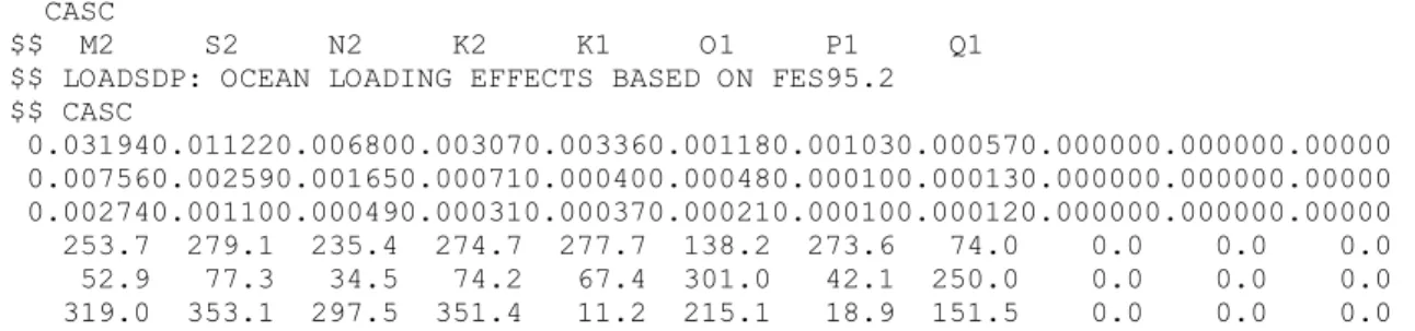
Table 4.1

for Cascais... 30

Table 4.2

Table 6.1

Table 6.2 Velocities computed for each baseline for the strategy E and the standard deviation (agreement) between the 5 implemented strategies in mm/year... 45

Table G.1 Velocities computed for each baseline in mm/year for the strategy A. ... 100

Table G.2 Velocities computed for each baseline in mm/year for the strategy B... 101

Table G.3 Velocities computed for each baseline in mm/year for the strategy C. ... 102

List of Figures

Figure 1.1 Agreement between directions and rates averaged over seven years of GPS

data and those given by the plate kinematic model NNR NUVEL1A... 2

Figure 2.1 Corresponding continent’s coastlines and location of several fossil plants and animals on present-day continents... 5

Figure 2.2 An observed magnetic profile matched by a calculated profile. ... 6

Figure 2.3 The main tectonic accidents in the studied Northeast Atlantic area... 8

Figure 2.4 Distribution of epicenters in the studied area. ... 8

Figure 2.5 Network map. ... 10

Figure 2.6 Maspalomas (left) and Villa Franca (right) stations panoramic views. ... 11

Figure 2.7 Cascais (left) and Lagos (right) stations panoramic views. ... 12

Figure 2.8 Santa Maria (left) and Graciosa (right) stations panoramic views. ... 13

Figure 3.1 Basic GPS positioning. ... 14

Figure 3.2 Geometry of the receiver-satellite double difference. ... 18

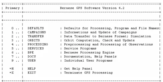
Figure 4.1 Menu system top level: groups of programs. ... 20

Figure 4.2 2002 campaign directory structure... 21

Figure 4.3 Panel 0.3.1 – General Dataset Names... 22

Figure 5.1 Process Control Script flow chart. ... 32

Figure 5.2 Entries in the Process Control File. Parts of the constructed Process Control File. ... 33

Figure 5.3 PANEL 1.5.1 – Filename Parameters for Automatic Processing... 35

Figure 5.4 PANEL 6.1 – BPE: Select PCF file (Panel Editing Tool). ... 36

Figure 5.5 PANEL 6.4.1.1 – BPE normal session processing: input options. ... 37

Figure 5.6 Entries in the constructed Process Control File... 38

Figure 5.7 Flow chart of the implemented automated system. ... 40

Figure 6.1 Time series of the baseline VILL – MADR... 46

Figure 6.2 Time series of the baseline VILL – GAIA. ... 47

Figure 6.3 Time series of the baseline MADR – GAIA... 47

Figure 6.4 Time series of the baseline VILL – CASC. ... 48

Figure 6.5 Time series of the baseline MADR – CASC... 48

Figure 6.6 Time series of the baseline VILL – OALN. ... 49

Figure 6.7 Time series of the baseline MADR – OALN... 49

Figure 6.8 Time series of the baseline VILL – OALS. ... 50

Figure 6.10 Time series of the baseline VILL – LAGO... 51

Figure 6.11 Time series of the baseline MADR – LAGO. ... 51

Figure 6.12 Time series of the baseline VILL – SFER. ... 52

Figure 6.13 Time series of the baseline MADR – SFER... 52

Figure 6.14 Time series of the baseline VILL – IMMA. ... 53

Figure 6.15 Time series of the baseline CASC – IMMA. ... 53

Figure 6.16 Time series of the baseline VILL – MAS1. ... 54

Figure 6.17 Time series of the baseline CASC – MAS1... 54

Figure 6.18 Time series of the baseline VILL – SMAR... 55

Figure 6.19 Time series of the baseline CASC – SMAR. ... 55

Figure 6.20 Time series of the baseline VILL – PDEL... 56

Figure 6.21 Time series of the baseline CASC – PDEL. ... 56

Figure 6.22 Time series of the baseline VILL – GRAC... 57

Figure 6.23 Time series of the baseline VILL – FLOR... 57

Figure 6.24 Time series of the baseline IMMA – SMAR... 58

Figure 6.25 Time series of the baseline MAS1 – SMAR. ... 58

Figure 6.26 Time series of the baseline IMMA – PDEL... 59

Figure 6.27 Time series of the baseline MAS1 – PDEL. ... 59

Figure 6.28 Time series of the baseline IMMA – MAS1. ... 60

Figure 6.29 Time series of the baseline SMAR – PDEL... 60

Figure C.1 Example of an UTEQC input file... 85

Figure C.2 UTEQC output file (batch) for the conversion and compression operations... 86

Figure C.3 UMUDNO input file example... 87

Figure C.4 UMUDNO output file and batch file for the precise orbital files name alteration. ... 87

Figure F.1 Strategy A outliers time series. ... 98

Figure F.2 Strategy B outliers time series... 98

Figure F.3 Strategy C outliers time series. ... 98

Figure F.4 Strategy D outliers time series. ... 99

Figure F.5 Strategy E outliers time series... 99

List of Acronyms

BPE Bernese Processing Engine BSW Bernese Software

EPN EUREF Permanent Network EUREF European Reference Frame

FCUL Faculdade de Ciências da Universidade de Lisboa GPS Global Positioning System

GPST GPS Time

IAG International Association of Geodesy IGP Instituto Geográfico Português IGS International GPS Service

ITRF International Terrestrial Reference Frame NAVSTAR Navigation System Time and Ranging PCF Process Control File

PCS Process Control Script PID Process Identification

RINEX Receiver Independent Exchange

SCIGN South California Integrated GPS Network SLR Satellite Laser Ranging

UNAVCO University NAVSTAR Consortium UTC Universal Time Coordinated VLBI Very Long Baseline Interferometry WGS84 World Geodetic System 1984

Acknowledgements

My gratitude is to the International GPS Service, the European Reference Frame, the Instituto

Geográfico Português and the Faculdade de Ciências da Universidade de Lisboa for the GPS data

made available and without which this study could not be made.

A very particular thanks to Dr. Virgílio Mendes for his patience, support and orientation. His reviews of the draft text significantly improved this dissertation. Certainly this study would be more complicated without his guidance.

Many thanks to Dr. Pierre Fridez for his help solving some initial software problems. Many thanks to Dr. José Madeira for his help and review about geodynamics.

I would like to extend my appreciation to the Examining Board (Dr. Joaquim Pagarete, Dr. Nuno Lima, Dr. João Matos, Dr. José Madeira and Dr. Virgílio Mendes) for their valuable suggestions and comments made on the draft manuscript.

Thanks to my colleagues Eng. Vitor Charneca, Eng. Ana Lopes and Eng. Fernando Martins. Their friendship, interest and support are greatly acknowledged. Through them I extend my thanks to the Escola Superior de Tecnologia da Universidade do Algarve.

I whish to thank my wife Andreia for her love and support.

My endless gratitude is to my parents, Maria Francisca and António Prates, for their love and support. Making them proud is always motivating. Through them I extend my thanks to all my friends and family.

1 Introduction

The present text is a dissertation submitted in partial fulfillment of the requirements for the degree of Master of Sciences in Ciências e Engenharia da Terra at the Faculdade de Ciências da

Universidade de Lisboa and describes the development of an Automated GPS data Processing

System using the Bernese GPS Software 4.2, specifically the Bernese Processing Engine. MOTIVATION

Today’s plate motion is tracked directly by means of ground-based or space-based geodetic measurements. In the 1970’s, the increase of space geodesy or space-based techniques made possible to repeatedly measure the surface of the Earth for changes. By measuring distances between carefully selected locations or stations it is possible to determine if there has been movements between plates and within plates.

Three of the most used space geodesy techniques are the Very Long Baseline Interferometry (VLBI), based on quasi-stellar extragalactic radio sources, the Satellite Laser Ranging (SLR) by laser pulses reflected on satellites, and the Global Positioning System (GPS) that utilizes radio signals emitted by satellites. For the measuring of Earth’s crustal motions, the most popular, convenient and cost effective of these techniques is the GPS [UNAVCO, 2003].

In 1994 the International Association of Geodesy (IAG) sponsored the beginning activities of the International GPS Service for Geodynamics, today simply International GPS Service (IGS), based on a large number of stations internationally distributed and on eight global Analysis Centers with the mission of data processing and analysis.

Space-geodetic data show that plate movements directions and rates averaged over several years compare well with plate kinematic models based on the directions and rates averaged over millions of years, considering magnetic reversals among other data, like for example the NNR NUVEL1A [DeMets et al., 1994], as illustrated in Figure 1.1.

In the last years, the increase in permanent GPS stations located worldwide made clear that the time consuming standard data processing tasks needed to be performed automatically. This kind of approach became a standard strategy for the International GPS Service Analysis Centers and their experience passed to the regional networks processing groups.

In Portugal, several permanent GPS stations were created lately, some maintained by public institutions to support the scientific community and standard surveying applications, others by universities and research laboratories. The resulting GPS data can play an important role in geodynamic studies, motivating the implementation of an automated system.

Such an automated system will be of key importance to ease the processing and analysis of the data collected by a network incorporating the permanent GPS stations maintained by the

Faculdade de Ciências da Universidade de Lisboa (FCUL). The primary goal of such network and

subsequently of the automated system is the GPS data analysis to reach a better geodynamic understanding of the region of the Northeast Atlantic, where three tectonic plates meet.

Figure 1.1 Agreement between directions and rates averaged over seven years of GPS data and those given by the plate kinematic model NNR NUVEL1A (After GFZ Potsdam [2003]).

OVERVIEW

High-precision GPS information is provided by continuously operating GPS tracking stations and data centers, under the auspices of the International GPS Service. The IGS provide crucial tracking data from their affiliated stations dispersed worldwide, high accuracy satellite orbit and clock data, Earth rotation parameters, a unified reference frame of station velocities and coordinates, and ionospheric information [IGS, 2003]. The global distribution of IGS stations is thus vital for regional networks geodynamic studies.

One example of regional networks is the South California Integrated GPS Network (SCIGN), whose major objectives are to provide coverage for estimating earthquake potential, identify active blind thrust faults and evaluate models of compressional tectonics, and measure local variations in strain rate and permanent crustral deformation not detectable by seismographs [Hudnut et al., 2001]. All stations in this particular network are affiliated to the IGS.

In Europe, taking benefit of the increasing number of permanent GPS stations, the European Reference Frame (EUREF) based on GPS measurements was established. The stations form the so-called EUREF Permanent Network (EPN), whose projects include time series screening for geokinematics and data support for other regional networks [EUREF, 2003].

Several other regional networks can be found throughout the globe, some of them using their own stations and thus increasing the number of permanent GPS stations worldwide.

Some GPS networks and different research groups have developed studies in the Northeast Atlantic area targeted by this dissertation. Although it is not intended to thoroughly indicate all scientific projects working in the study area, some will be presented.

One project is the so-called Atlantic and Mediterranean Interdisciplinary GPS Observations (AMIGO) [Elósegui et al., 1999]. Among others, the goal of this research group is to develop a coherent picture of the entire Mediterranean tectonics by combining GPS-geodynamic studies of the western network (including the east Atlantic region between the Azores Islands and the Strait of Gibraltar) with the results from ongoing research in the eastern Mediterranean and neighboring regions (including northern Europe, the Middle East, and East Africa). Several projects do not use permanent GPS stations; hence the sites are occupied in periodic campaigns. The Trans-Atlantic Network for Geodynamics and Oceanography (TANGO) uses this kind of approach in the observation of sites placed in the Azores Archipelago, where just 2 stations are permanent [Fernandes et al., 2002]. The objective of this research group is to establish a coherent description of the velocity field in a group of stations located along the Azores Islands and to define plate boundaries in the Azores region.

Recently, other project was proposed supported on the campaigns approach to evaluate the Tectonic, Volcanic, and Landslide Displacements at Faial, Pico, and S.Jorge (Azores) using GPS (DISPLAZOR) [Mendes et al., 2002]. The objective of this research group is to quantify the surface deformation of tectonic, volcanic and landslide origin.

CONTRIBUTION

As only the AMIGO project includes the FCUL group of stations, in this study an independent analysis of the FCUL stations data is offered. Furthermore, with this study’s results perhaps added information about the kinematic behavior of the involved tectonic plates might be considered in future geodynamic revisions, since as a by-product of the implementation of the automated system some time series of baselines will be presented and analyzed.

In addition, the analysis of the 5 studied processing strategies will confer a perspective of the influence of diverse approaches. This assessment will serve as basis for future developments of the implemented automated system, resulting in a robust GPS data processing tool.

Furthermore, the knowledge acquired with the automated system implementation, using the Bernese Processing Engine, will be made accessible, contributing for the dissemination of this automated solutions and helping other projects to produce results in a straightforward way. OUTLINE

Chapter 1 – Introduction – In this chapter the motivation for this study, a slight overview of the global and regional networks for GPS data analysis for geodynamics, the contribution of this study, and the outline of this dissertation are presented.

Chapter 2 – Global Positioning System Network for Geodynamics – In this chapter a small revision of the Plate Tectonics geodynamic theory will be presented; the Northeast Atlantic tectonics is discussed and a short presentation of the network of permanent GPS stations used for the study of the mentioned region is given.

Chapter 3 – Global Positioning System – In this chapter a slight overview of the GPS is given and a number of particular terms that will be used in the subsequent chapters to explain the processing strategies are introduced.

Chapter 4 – Bernese Software – In this chapter the standard sequence of operations used by the Bernese GPS Software 4.2 to compute the data of a regional network is presented and the 5 studied processing strategies are described.

Chapter 5 – Bernese Processing Engine – In this chapter a description of the implementation of the automated processing system on the Bernese Processing Engine and details about the assembled automated system are given.

Chapter 6 – Automated Processing - Results – In this chapter the results about the processing strategies evaluation are given and an analysis of the most significant time series of baselines computed by the automated system is presented.

Chapter 7 – Conclusions and Outlook – In this last chapter some conclusions and suggestions for future development of the automated system and data analysis are given.

2

Global Positioning System Network for Geodynamics

“This must be left to the geodesists. I have no doubt that in the not too distant future we will be successful in making a precise measurement of the drift of North America relative to Europe.”

Alfred Wegener, 1929 [UNAVCO, 2003]

In 1912, Alfred Wegener introduced the idea that the Earth’s outermost layer is fragmented into several plates moving relative to one another. Wegener’s theory, called Continental Drift, was based on what it seem to him to be the notable fit of the South America and the African continents, noted centuries earlier by Abraham Ortelius, a mapmaker [Lindeberg, 2001]. Wegener considered as well the occurrence of unusual geologic structures and of animal and plant fossils on the matching coastlines (Figure 2.1). According to him, these related fossils and the finding of tropical plant fossils in the Antarctica, showing that this continent drifted from near Equator to Polar Regions, were explained by the Continental Drift theory.

Figure 2.1 Corresponding continent’s coastlines and location of several fossil plants and animals on present-day continents [Lindeberg, 2001].

Nevertheless, Wegener’s theory was weakened by unsatisfactory explanation of what kind of forces could be powerful enough to shift large continental masses over large distances, as he suggested that the continents simply plowed through the ocean floor.

In the 1950’s, the use of magnetic instruments led to the detection of odd magnetic variations across the ocean floor. This discovery was not surprising, as it was known that the magnetite in basaltic rocks may well locally distort compass readings and that when magma cools to form a solid volcanic rock the alignment of the magnetite grains record the Earth’s magnetic orientation at the time of cooling.

As further seafloor was mapped a magnetic pattern became recognizable. Alternating stripes of magnetically different rocks were laid out in rows on either sides of a mid ocean mountain chain known as mid-ocean ridge: one stripe having the present-day magnetic orientation of the Earth (normal magnetic polarity) and the neighboring stripe with the opposite orientation (reversed magnetic polarity). By 1966 the magnetic reversals history for the last 4 million years was reconstructed using a dating technique based on the isotopes of potassium and argon. When assuming that the ocean floor spread away from the mid ocean ridge at a rate of a few centimeters per year, the calculated magnetic reversals showed a notable correlation with the magnetic striping pattern found on the ocean floor (Figure 2.2).

Figure 2.2 An observed magnetic profile matched by a calculated profile [Lindeberg, 2001].

Though, if the Earth’s crust is expanding along the oceanic ridges then it should be shrinking elsewhere. Harry Hess introduced the notion that the seafloor eventually descends into very deep and narrow canyons known as oceanic trenches detected in earthquakes concentration maps, in the same way the spreading ridges can be [Lindeberg, 2001].

The current plate motion is monitored directly by using geodetic measurements, favored by the increase of permanent GPS stations worldwide, since this is the most cost effective of the space-geodetic techniques. In fact, the GPS data has shown that plate motions averaged over several years compare well with plate kinematic models [GFZ Potsdam, 2003].

In this chapter, after a small revision of the evidences supporting the geodynamic theory of

Plate Tectonics, a brief discussion of the Northeast Atlantic tectonics will be given, along with

the description of the GPS network covering the mentioned area and used in this study.

2.1 Northeast

Atlantic

Tectonics

The GPS network used in this study is located in an area of great geological importance, as it occupies three different tectonic plates (the North American, the Eurasian and the African) that form one triple junction within this Northeast Atlantic area (Figure 2.3).

The North American plate is detached from the other two by the mid-Atlantic ridge, whereas the Azores-Gibraltar fault zone, that stretches through the Mediterranean, splits the Eurasian and the African plates. The triple junction is located in the Azores Archipelago region.

The Western group of the Archipelago is separated from the Central and Eastern groups by the mid-Atlantic ridge, meaning that the Corvo and Flores islands are in the North American plate whereas the other Azorean islands are standing in a broad deformation zone between the Eurasian and the African plates [Madeira, 1998].

Recent spreading rate of the mid-Atlantic ridge continues at near 24 mm/year according to the plate kinematic model NUVEL1 [DeMets et al., 1990].

The boundary between Eurasia and Africa in the Azores area remains unclear. According to Miranda et al. [1991], the triple point has moved north along the mid-Atlantic ridge from its intersection with a deactivated fracture south of the Archipelago to its recent position, giving origin to several faults that embrace the region of the central and oriental island groups from a point in the Azores-Gibraltar fault toward the mid-Atlantic ridge.

Figure 2.3 The main tectonic accidents in the studied Northeast Atlantic area.

The instrumental epicenters distribution in the Azores (Figure 2.4) illustrates that the broad deformation zone separating the Eurasian and the African plates has the alignment between S. Miguel and S. Jorge. In this broad deformation zone Madeira and Ribeiro [1990] suggested a fault zone, named S. Jorge Leaky Transform, with the combination of ridge opening of near 4.0 mm/year, and dextral transform of about 1.1 mm/year [Ribeiro, 2002]. This strain regime has been confirmed by geodetic methods [Pagarete et al., 1998].

The Azores-Gibraltar fault zone between the eastern tip of the broad deformation zone and the Gorringe Bank, southwest of Portugal, has the name of Gloria fault. This sector has pure dextral transform motion due to the distinct Eurasian and African ridge spreading rates, and for that reason with modest epicenter distribution [Ribeiro, 2002].

At the Gorringe Bank the Eurasian and African plates collision zone is reached. Towards the Mediterranean the convergence rate increases. Present-day convergence between these two plates continues at the rate of 4.0 mm/year [Ribeiro, 2002], according to the plate kinematic model NUVEL1 [DeMets et al., 1990].

Furthermore, the instrumental seismicity shows epicenter distribution along the west Iberia margin, which is strange for a passive margin. This observation, additionally supported by neotectonic data, leads to the possibility that the west Iberia margin is in a state of transition from passive to active, being a case of oceanic trench formation and subduction initiation. As indicated by Ribeiro [2002], perhaps nucleating at the Gorringe Bank, subduction has already started in the southern sector and is propagating northwards.

From the viewpoint of active tectonics, the Iberian Peninsula is a small, nonetheless massive, continental block surrounded by more mobile belts [Ribeiro, 2002]. In fact, the Iberia tectonic regime suggests progressive independent movement from the stable Eurasia at rates below 1.0 mm/year, as inferred by geodetic data [Elósegui et al., 1999].

According to Ribeiro [2002], the northern boundary of the Iberia microplate is sited along the Cantabrian-Pyrenean range by extending the Pyrenean fault zone westwards.

2.2 Network

Description

The network established for this study includes almost all permanent GPS stations situated in Portuguese territory. Besides those, the network was complemented with some IGS stations, with known coordinates in the International Terrestrial Reference Frame (ITRF).

The stations located in Portuguese territory are either maintained by the Faculdade de Ciências

da Universidade de Lisboa (FCUL) or by the Instituto Geográfico Português (IGP). Several of these stations are IGS and/or EUREF stations.

As shown in Figure 2.5, the stations are disseminated through the Iberian Peninsula and the Azores, Madeira and Canaries Archipelagos. The area covered has great geological meaning, as the stations occupy three diverse tectonic plates (Eurasian, African and North American) and can therefore provide information about their relative movements.

Figure 2.5 Network map.

The considered IGS stations are Madrid (MADR), Maspalomas (MAS1), San Fernando (SFER), Villa Franca del Campo (VILL) and Ponta Delgada (PDEL).

Madrid station is situated in Spain and is maintained by the Jet Propulsion Laboratory. Its activity was initiated in December 1989 and presently has an Ashtech Z-XII3 receiver with a Rogue Tantenna. All data used in this study was acquired by this hardware.

The Maspalomas station (Figure 2.6) was established in April 1994 and is maintained by the European Space Operations Center. This station is sited in the Canaries Archipelago, Spain. It utilizes an Ashtech Z-XII3 receiver since December 2000, but maintains a Rogue T antenna since April 1996.

The San Fernando station, situated in southern Spain, is maintained by the Real Instituto y

Observatório de la Armada. Its activity was initiated in December of 1995. A Trimble 4000SSE

receiver and a Trimble 29659 antenna acquired all data used in this study.

Villa Franca del Campo station (Figure 2.6) was created in November 1994 by the European Space Operations Center. It is located near Madrid, Spain. Presently it uses an Ashtech Z-XII3 receiver and a Rogue T antenna. In this study, this station was chosen as the data processing reference station, since it has lesser data failures than others and stable ITRF coordinates. Ponta Delgada station belongs to the Instituto Geográfico Português. It is located in the Azores Archipelago, Portugal. It began its activity in January 2000 with a Leica AT504 antenna, but the receiver was changed from a Leica CRS1000 to a Leica RS500 in December 2002.

The EUREF stations used in this study are Cascais (CASC), Lagos (LAGO) (see Figure 2.7) and Vila Nova de Gaia (GAIA). Maspalomas, San Fernando, Villa Franca del Campo and Ponta Delgada are EUREF stations as well, which were already described.

The former Instituto Português de Cartografia e Cadastro and now Instituto Geográfico Português, established these three stations. Cascais initiated its activity in March 1997 and the other two in January 2000. Currently all of them use a Leica RS500 receiver and a Leica AT504 antenna. These Portuguese stations are situated in the coastline: one in the center (Cascais), one in the south (Lagos) and one in the north (Vila Nova de Gaia).

Figure 2.7 Cascais (left) and Lagos (right) stations panoramic views.

The stations here named FCUL stations were installed and are maintained by the Faculdade de

Ciências da Universidade de Lisboa. This network includes Flores (FLOR), Graciosa (GRAC) and

Santa Maria (SMAR), sited in the Azores Archipelago, Instituto de Meteorologia da Madeira (IMMA), sited in the Madeira Arquipelago, and Observatório Astronómico de Lisboa Norte (OALN) and Observatório Astronómico de Lisboa Sul (OALS), sited in Portugal mainland. The oldest of FCUL stations is the Instituto de Metereologia da Madeira, established in March 1999. Presently uses a Trimble 4000SSI receiver and a Trimble 29659 antenna.

The Observatório Astronómico de Lisboa Norte station’s activity initiated in May 1999. Since then it uses an Ashtech Z-XII3 receiver and an Ashtech 700936E antenna.

Flores and Santa Maria were installed in 1999 and Graciosa (Figure 2.8) was installed in 2002. All stations use Leica CRS1000 receivers and Leica AT504 antennas. Unfortunately, these sites have software and hardware problems that result in poor data availability.

Figure 2.8 Santa Maria (left) and Graciosa (right) stations panoramic views.

The Observatório Astronómico de Lisboa Sul station began its activity in 2002. It uses a Leica CRS1000 receiver and a Leica AT504 antenna.

In this chapter a short revision of the Plate Tectonics geodynamic theory was presented as a preface to the Northeast Atlantic tectonics discussion and the permanent GPS network slight presentation. In the next chapter, an overview of the Global Positioning System is given and some particular terms are introduced.

3

Global Positioning System

In late 1973, the United States Department of Defense begun the development of one system based on artificial satellites intended to grant precise time and navigation, 24 hours a day, anywhere in the world and under any atmospheric conditions.

This system, named Global Positioning System (GPS), is a one-way radio system emitting in two frequencies that utilizes a nominal constellation of 24 satellites, from which the distances between a receiver and the known positions of satellites can be measured.

The receiver position is given by the intersection of three spheres with a radius equal to three measured distances, each one centered on its own satellite. Actually four are required, since time has to be precisely computed as well (Figure 3.1).

Figure 3.1 Basic GPS positioning [Trimble, 2001].

The two frequencies used by GPS are known as Link 1 (L1) transmitted at 1575.42 MHz and Link 2 (L2) transmitted at 1227.60 MHz. Both frequencies have modulated binary sequences or codes, different for each satellite.

Beyond 2005, a third frequency will be available located at 1176.45 MHz. The new signal will improve the robustness and reliability of GPS, and moreover support many new applications that benefit from measurements on several frequencies.

The L1 frequency has two modulated binary codes, one known as Clear/Acquisition (C/A) consisting of a sequence of 1023 digits at the rate of 1.023 MHz, and a second having a total of _{2.34 ×10}14_{digits emitted at the rate of 10.23 MHz known as Precise (P). From these two,} only the P code is modulated in the L2 carrier. These two codes serve to identify the emitting satellite and provide, through the comparison with a replica generated by the receiver, the signal traveling time from the emitting satellite to the receiver.

Both frequencies have the satellites orbits or ephemerides encoded as well. This navigation message has 1500 binary digits emitted at the rate of 50 Hz. The 24 satellites are divided in 6 orbital planes separated about 60º in longitude and having an inclination of 55º with respect to the Equator. The satellites orbital period is near 12 sidereal hours.

Besides, the system uses its own time scale. It is known as GPS Time (GPST) and is based on the atomic clocks of the system control stations (Colorado Springs, Kwajalein, Diego Garcia, Ascension and Hawaii) and of the satellites. This time scale is analogous to the Coordinated Universal Time (UTC), nevertheless without the leap seconds introduced in the UTC, in order to keep a close relation between the UTC atomic time scale and the Earth’s rotation. With this time scale, the concepts of GPS Week and of GPS Second were introduced. The GPS Week is counted since January-06-1980, and the week day is valued from 0 (Sunday) to 6 (Saturday). The GPS Second is counted from the 0 hours of each week’s Sunday.

Furthermore a coordinate system was established for the satellites positioning. This system is known as the Word Geodetic System 1984 (WGS84). However, the IGS pos-processed satellite ephemerides, commonly used to process GPS data for geodynamic studies, are based on the ITRF coordinate frames established by the IGS stations network. Since the stations move with the crustral motion, the ITRF coordinate system suffers slight adjustments from time to time. The last change in the ITRF system was introduced in 2002 and was named ITRF2000. There is a mathematical relation that makes possible to transform among these coordinate systems. In this chapter after this slight presentation of the Global Positioning System it will follow an introduction of some GPS particular terms and basic processing strategies.

3.1 Observables

The distance between the satellite and the receiver can be given by using the time difference between the emission of the code and its reception. If the receiver and satellite clocks were synchronized and the propagation medium was the vacuum, the speed of light in vacuum (c) and the code travel time (dτ) would give the satellite-receiver range ρ by

τ

ρ=c ⋅d , (3.1)

Yet, both receiver and satellite clocks are often unsynchronized with the GPS Time scale and the propagation medium is the Earth’s atmosphere, resulting a measured travel time (dτ'). If we take into account the effects of the ionized atmosphere (di) and the electrically-neutral atmosphere (dn), and the synchronization errors of receiver clock (dT) and satellite clock (dt), the equation for the so-called pseudorange (p=c⋅dτ') will be written as

(

)

c

p=ρ+ ⋅ − + + . (3.2)

The distance between the satellite and the receiver ρ can also be computed using the number of complete phase cycles from the satellite to the receiver and the phase difference between the emitted and received signals,

(

)

⋅ =λ φ

ρ , (3.3)

where λ is the wavelength, φ is the phase difference in cycles plus a cycle count performed by the receiver until signal lock and N is the unknown total of phase cycles from satellite to receiver less the receiver cycle count that is identified as phase ambiguity, cycle ambiguity or simply ambiguity.

Yet, like the pseudorange observable, the phase difference measured (φ‘) by the comparison of the received signal (satellite clock dependent) with its replica (receiver clock dependent) is time dependent, and suffers from atmospheric refraction. Hence, the equation for the phase observable (Φ=−λ⋅φ') will be written as

(

)

c⋅ − + ⋅ − +

+

=ρ λ

Φ . (3.4)

The ionospheric effect signal modification is due to a characteristic of this layer that increases the velocity of the carrier phase and delays the modulated group signal.

Also note that the theoretical range ρ is given by the satellite and the receiver coordinates,

2 2 2 _{Y Z} X +∆ +∆ ∆ = ρ . (3.5)

3.2 Observables

Differences

The errors that affect the GPS observables measured simultaneously by two receivers not far apart show some correlation. These systematic errors might therefore be either eliminated or minimized by differencing the observables.

Since the phase measurements give more precise ranges than the time (code) measurements, although the unknown ambiguity has to be estimated, the differencing of observables will be presented using phase. Yet, the same can be made using pseudorange measurements.

The difference of observables can be performed between two receivers, p and q, that use the

same satellite, giving the so-called single difference between receivers

p Φ = ρp +c ⋅dt −c ⋅dTp +λ⋅Np −dip +dnp q Φ − = −ρq −c ⋅dt +c ⋅dTq −λ⋅Nq +diq −dnq Φ ∆ = ∆ ρ +c ∆⋅ dT +λ⋅∆N −∆di +∆dn (3.6)

Given that the same satellite is observed, the same satellite clock error affects both equations, so the difference eliminates this bias. The atmospheric effects are similar for short baselines, since identical paths are taken through the atmosphere, so these errors are minimized.

The difference of observables can be performed among two satellites, i and j, observed by the

same receiver, giving the so-called single difference between satellites

i Φ = _ρi _{+c ⋅dt}i _{−c ⋅dT +λ⋅N}i _−dii _+dni j Φ − = _−ρj _{−c ⋅dt}j _{+c ⋅dT −λ⋅N}j _+dij _−dnj Φ ∇ = ∇ ρ +c ∇⋅ dt +λ⋅∇N −∇di +∇dn (3.7)

In this difference the receiver clock error is eliminated, but the atmospheric delays are only minimized if the satellites have similar elevation angles, so that similar path lengths through the atmosphere are taken by both carrier waves.

The difference of observables can be performed between two observation epochs, k and n, of

the same satellite-receiver par, giving the so-called single difference between epochs

k Φ = ρk +c ⋅dtk −c ⋅dTk +λ⋅N −dik +dnk n Φ − = −ρn −c ⋅dtn +c ⋅dTn −λ⋅N +din −dnn Φ δ = δρ +c⋅δdt +c⋅δdT −δdi +δdn (3.8)

The previous single difference only holds if there is no loss of signal between the two epochs, meaning that the phase ambiguity is the same for both epochs, and as a result the difference eliminates this bias. If there is signal loss the ambiguities difference must be computed, as its value is different from zero. In any case, for epochs not far apart the atmospheric delays are minimized, as the atmospheric conditions do not change suddenly.

In fact, the combined results concerning the biases elimination or reduction can be attained if more than one single difference is used. Thus, instead of the differences previously presented double differences can be achieved by combining two single differences.

The double difference receiver-satellite that combines the observations from two receivers to two satellites is the most used (Figure 3.2), since it eliminates all the clock errors and reduces the atmospheric effects, being written as

dn di N ∆ ∆ ∆ ∆ ∆ =∇ + ⋅∇ −∇ +∇ ∇ Φ ρ λ (3.9)

For geodetic applications the phase double differences receiver-satellite are commonly taken as basic observations, nevertheless the ambiguities have to be estimated.

Figure 3.2 Geometry of the receiver-satellite double difference (After Schaer [1999]).

The triple difference given by differencing two epochs of receiver-satellite double differences is less used for positioning purposes, as it significantly reduces the number of observations. Yet, it is of extreme utility to find signal losses or cycle slips. In fact triple difference solutions are biased with the resulting non-zero ambiguities difference; therefore, they are not similar to the solutions determined when no signal loss or cycle slips has occurred, which have an ambiguity difference equal to zero.

3.3

Linear Combination of Observations

The linear combination of observations uses the same measurement type, but from different frequencies, for dual-frequency receivers.

Like in the last section, the linear combination of observations will be presented using phase measurements. Nevertheless, pseudorange measurements can be used as well.

Considering the two phase observables, in L1 and L2, for the same satellite receiver pair, any linear combination is written by

2 L 1 L ab a φ b φ φ = ⋅ + ⋅ , (3.10)

where a and b are coefficients of a specific linear combination.

The number of linear combinations is unlimited; however they are only used if they offer any advantage. The advantages are in general the ease in ambiguity resolution and the reduction of the ionized atmosphere effects.

For ambiguity resolution the most used combination is the wide-lane given by

2 L 1 L 1 1 φ φ φ_∆ = ⋅ − ⋅ . (3.11)

This combination has a larger wavelength than both L1 and L2, though the associated noise is close to 6 times the noise of the original frequencies [Mendes, 1995]. The larger wavelength makes easier to solve the number of complete cycles that affects the phase measurements. It is known that the ionized atmosphere delay is frequency dependent, making possible to eliminate this delay if a combination of both frequencies is used. In fact, the ionosphere-free combination reduces the ionospheric delay to a great extent and is normally used to compute large baselines. For short distances between receivers is not so advantageous given that it has about 3 times the noise of the original waves [Mendes, 1995].

The ionosphere-free linear combination is given by

2 L 2 1 L 2 2 L 1 L LC f f 1 φ φ φ = ⋅ − ⋅ , (3.12)

where f_L1 is the L1 frequency and f_L2 is the L2 frequency.

In this chapter a small presentation of the Global Positioning System was given and some GPS particular terms and basic processing strategies where introduced. In the next chapter the usual sequence of operations of the Bernese GPS Software 4.2 to compute the data from a regional network is presented and the 5 studied processing strategies are described.

4 Bernese

Software

The processing part of Bernese GPS Software 4.2, developed at the University of Bern, consists mainly of Fortran programs that run in batch mode, not requiring any user interaction during their execution time. Nevertheless, a menu system is accessible to help setting the options for programs, preparing data and auxiliary files, and keeping track of the output files.

In order to navigate through the preparatory and processing programs, a sequence of panels guide from the top level groups of programs (see Figure 4.1), through program’s input files preparation and options selection, to program execution and output files management. Three different types of panels are identifiable in the menu system: the program panels for program selection, the data panels for input files and options designation, and the help panels for additional information about programs options.

Figure 4.1 Menu system top level: groups of programs.

Bernese software uses directory structures placed in four main areas: the program area, for the software and general support files, the data area, for the campaign data and auxiliary files, the

user area, for user specific options, and the temporary area, for temporary files. The locations of these areas are defined in the LOADGPS script that starts the Bernese software (the LOADGPS script is created during the software installation – see Hugentobler et al. [2001] for details). This chapter describes the basic sequence of the Bernese programs used to process a regional network, and the processing strategies considered in this study.

4.1 Processing

Sequence

The first procedure is the campaign setting. Basically, the campaign duration and directory structure needed by the Bernese software are established. The campaign has to be created (or identified, if already existent) and, if the necessary subdirectories are inexistent, they need to be created too (see Figure 4.2). Each campaign directory structure, named campaign area, will be created within the data area defined in the LOADGPS script. To achieve both tasks, Panel 1.1 and Panel 1.2 are used, respectively.

Figure 4.2 2002 campaign directory structure.

In addition, session duration must be defined by filing Panel 1.3.2; the wildcard string ???O should be used to represent any session (day of the year), and 24-hour sessions should be set so that all available data may be processed.

To process GPS data, several auxiliary files are needed. The names of some of these files have to be specified in Panel 0.3.1, particularly the name of the Earth’s rotation file (ERP) and the satellite manoeuvers file (CRX) need to be checked (see Figure 4.3).

The second procedure is the data conversion from Receiver Independent Exchange (RINEX) ASCII format to the Bernese binary format. In this process, the Bernese software can modify the RINEX header information, using translation tables for station names (STA), receiver and antenna types (TRN), and antenna heights (HTR). A RINEX file will be discarded if its header information is different from the one expected in the translation tables.

The translation tables for station names and antenna heights require to be located in the STA subdirectory in the campaign area, whereas the receiver and antenna translation table must be located in the GEN directory in the program area.

Figure 4.3 Panel 0.3.1 – General Dataset Names.

The translation tables for the selected stations can be found in Annex B.

Unfortunately, due to receiver software limitations in the conversion to RINEX, FCUL stations header information was often incomplete, so it was necessary to correct this problem.

To alter the header information in those files the TEQC software was applied. This program, developed by UNAVCO (University NAVSTAR Consortium) is able to read binary and RINEX version 2 files from some receiver manufacturer, and convert those files into standard RINEX version 2 format. In the conversion process, the RINEX header information can be corrected. TEQC is executed from a shell command line. Therefore, a batch file can be created to execute several similar command lines and correct many data files. This batch file was written using a Fortran program (UTEQC) developed by the author.

A user manual for the UTEQC program can be found in Annex C.

The UTEQC program requires an input file with the header information of a specific station and the time period of data files to be corrected. In addition, standard file compression tools can be used (for data storage purposes). The input file information is used to write blocks of command lines for every data file into the batch file (see Annex C), to be then executed. The command lines are written for the LINUX operating system.

After FCUL stations data files correction, all RINEX files pertaining to a particular campaign require to be copied to the RAW subdirectory in the campaign area. Bernese data conversion (RINEX to Bernese) program (RXOBV3) is executed from Panel 2.7.1.

In the next procedure, satellite orbital information is converted for Bernese software use. For a regional campaign processing, IGS precise satellite orbits should be used. Two operations must be performed: precise orbits in the terrestrial system are converted in tabular satellite positions in the celestial reference frame, followed by the creation of standard orbits for each satellite using the tabular positions as pseudo-observations.

A standard orbit may be composed of one or more standard arcs, for a specified time interval each, given as particular solutions of the equations of motion that best fit the tabular satellite positions. The reference system conversion accounts for effects on the satellite’s orbit caused by Sun, Planets and Moon, also reflected in the Earth’s polar motion and ocean tides, whose effects can be furthermore considered.

In addition, a low degree polynomial for every satellite is customarily adjusted to the clock information from precise orbits files. Then, this polynomial may be used to compute satellite clock corrections for each observation epoch. A single 24-hours arc was used, as suggested in the Bernese GPS Software manual [Hugentobler et al., 2001], and two quadratic polynomials for 12-hours clock corrections each.

As previously stated, the Bernese GPS Software can consider the effects on the satellite’s orbit caused by Sun, Planets and Moon. In order to attain that, the needed planetary ephemerides in binary version must be retrieved from the Jet Propulsion Laboratory (JPL) anonymous ftp (ftp://nav.jpl.nasa.gov/ephem/export/unix/). The binary files are available in 50 years blocks, each block having the start year and the ephemerides type identified in the file name. If more than one file is required, then a Fortran program is offered to merge contiguous files. In this study, the JPL DE200 ephemerides were used (the corresponding binary file is located in the GEN directory in the program area with the name DE200.EPH).

The IGS precise orbits files must be copied into the ORB subdirectory, in the campaign area. The conversion to tabular satellite positions program (PRETAB) runs from Panel 3.2, whereas the standard orbits creation (ORBGEN) is executed from Panel 3.3.

A Fortran program (UMUDNO) was written to change the name of the IGS precise orbits file to the corresponding name required by the Bernese (see Annex C for details).

The pre-processing part is the next procedure, where the first operation is to attain receiver clock corrections with accuracy better than 1 µs.

It would be possible to determine these clock corrections as unknown parameters in the final least-squares adjustment, but this would increase considerably the number of parameters. Nevertheless, a priori clock corrections can be computed with sufficient accuracy using the ionosphere-free time (code) linear combination. In this study, every reached clock corrections were used in the corresponding epochs, although a low degree polynomial could be adjusted to them in order to resolve a posteriori smoother clock corrections.

The code processing for clock corrections program (CODSPP) runs from Panel 4.2.

Bernese software uses mainly phase double differences as basic observables. Hence, the next task is the creation of single differences (between receivers) and subsequent storage in files, which are used later to compute the double differences.

To attain the set of independent baselines used in single differences computation one criteria must be selected. The available criteria include the shortest baselines, the maximum number of single differences or a star configuration (all independent baselines formed using the most central station of the network as reference). User baseline choice is also available, introducing that information manually or through a definition file. A strategy using all possible baseline combinations (therefore linearly dependent) is also available. In this study, the used strategy was the one giving the maximum number of single differences.

The single differences program (SNGDIF) is executed from Panel 4.3.

Before the final adjustment, cycle-slip screening is performed. Cycle-slip is the name given to a leap in the phase measurement by an integer number of cycles caused by the loss of signal lock. When found, a cycle-slip is repaired if the integer leap number of cycles can be attained, marked as an outlier or a new ambiguity is introduced in the final least-squares adjustment. The methods used to detect cycle-slips consist in checking the observed phase value against the expected phase value estimated with a low degree polynomial and in inspecting triple difference solutions, because one cycle-slip only corrupts one triple difference solution. The cycle-slip screening program (MAUPRP) is executed from Panel 4.4.2.

The final procedure is the least-squares adjustment that leads to the positioning solution. The basic observables are phase double differences that are computed from the single differences created before the adjustment. Different processing strategies are possible and a number of those possibilities are discussed in the next section.

The final least-squares adjustment program (GPSEST) runs from Panel 4.5.

4.2 Processing

Strategies

The Bernese software uses phase measurements to compute the positioning solutions. Phase measurements are biased by systematic errors (satellite orbits, satellite clocks, propagation medium, receiver clocks, antenna phase center variations, etc.) and random errors. In the Bernese software all relevant systematic errors are carefully modeled.

The satellite orbits, satellite clocks and receiver clocks are computed prior to the positioning solution with double differences observations. The processing strategies vary basically in the approaches to determine the ambiguities, the ionospheric delay and the tropospheric delay. THE IONOSPHERIC DELAY

The traditional strategy to minimize the effect of the ionospheric delay consists on using the ionosphere-free combination. Because the ionosphere is a dispersive medium for microwave signals, the ionospheric delay is frequency dependent. An estimate of the ionospheric delay [Mendes, 1995] is given by TEC f 3 40 di= ₂. ⋅ , (4.1)

where f is the frequency of the carrier and TEC is the total electron content in a column with 1 _m2 _{of transversal section, along the satellite-receiver trajectory.}

For each linear combination given by the Equation 3.10, the ionospheric delay will be written as the sum of the original biases scaled by the respective coefficient,

TEC f 3 40 b TEC f 3 40 a di ₂ 2 L 2 1 L ⋅ ⋅ + ⋅ ⋅ = . . . (4.2)

Any linear combination that gives a null ionospheric delay is recognized as ionosphere-free combination. The typical ionosphere-free linear combination is written as

2 L 2 1 L 2 2 L 1 L LC f f 1 φ φ φ = ⋅ − ⋅ . (4.3)

In fact, the ionosphere-free combination only reduces the ionospheric delay, nevertheless the residual bias is lesser than 2 cm [Bassiri and Hajj, 1993]. In this study, the final solutions were attained using the ionosphere-free linear combination.

THE AMBIGUITIES

Every unmeasured integer cycle number or initial phase ambiguity is computed as real value in the least-squares adjustment. Solving the ambiguities means to assign the accurate integer numbers to the real values estimates. Even though the positioning solutions can be attained with the ambiguities as real values, the solutions tend to improve if they are resolved.

To solve for the ambiguities many strategies are known. From those accessible in the Bernese software, the selected ambiguity resolution strategy was the Quasi-Ionosphere-Free (QIF) (see Mervart [1995]). This approach allows solving directly the phase ambiguities of both L1 and L2 on long baselines, without using precise time (code) measurements and able to deal with larger ionospheric delays than the wide-lane method [Schaer, 1999].

Neglecting the troposphere bias, simplified double difference observation equations for the L1 and L2 phase observables (see Equation 3.9) are written as

1 1 1 L L L =ρ−di+λ ⋅N φ (4.4) 2 2 2 2 2 1 2 L L L L L di N f f _{⋅ + ⋅} − =ρ λ φ (4.5)

where di is the ionospheric delay in the L1 phase observable.

The L1 ionospheric bias can be computed slightly constrained, and pre-eliminated epoch by epoch [Schaer, 1999] or established by means of a regional ionosphere model supplied by the IGS [Mervart, 1995]. In this study, the first option was used.

The constraint to the ionospheric bias is imposed by an a priori value that may stem from any basic ionosphere model. The pre-elimination of every epoch-specific ionosphere parameters, epoch by epoch, is essential since after several epochs the number of ionospheric parameters becomes too large to handle the normal equation system.