Introduction
Studies of forest biomass are important for the assessment of net primary productivity and carbon storage, quantification of forest residues for commer-cial purposes (energy and f iber) and ecosystem nutrient recycling. These studies are of great impor-tance for the decision making of forest resource ma-nagement (Páscoa et al., 2004). The use of forest bio-mass for bioenergy is increasingly recognized in European countries as part of an integrated strategy aimed at mitigating climate change, improving safety renewable energy and forest fire prevention (Viana et al., 2012). A United Nations Framework Convention on Climate Change (UNFCCC) and, in particular, the Kyoto Protocol, also recognize the great importance of forest biomass and carbon and the need to monitor,
given its influence on the concentration of the atmos-pheric CO2.
Forest biomass can be accessed through two me-thods: the destructive method, which includes the quantification of weights and/or volumes of individual felled trees, through inventory techniques, and non-destructive methods where the estimation of the bio-mass (or volume) is supported by regression models, or, for large landscapes scales, by remote sensing tech-nology such as the Laser Imaging Sensor (Parresol, 2002, Picard et al., 2012). In most situations, the first method is reserved for the generation of data to ena-ble the development of the regression models, usually using allometric equations. The general expression is Y = a Xb, where Y represents the biomass or volume of the stem (or of other compartment), X usually refers to the diameter at 1.30 m, and a and b are the allome-tric constants. The allomeallome-tric relationship assumes that the biomass growth is proportional to the growth in diameter. When Y refers to stem volume, the value
ob-Biomass conversion and expansion factors are afected by thinning
Teresa Duque Enes
1,2* and Teresa Fidalgo Fonseca
31 Department of Forest Sciences and Landscape Architecture. University of Trás-os-Montes and Alto Douro. 5000-801 Vila Real, Portugal. 2 Centro de Estudos Florestais. Instituto Superior de Agronomia. Universidade
de Lisboa. Tapada da Ajuda. 1349-017 Lisboa, Portugal. 3 Department of Forest Sciences and Landscape Architecture. University of Trás-os-Montes and Alto Douro. 5000-081 Vila Real, Portugal
Abstract
Aim of the study: The objective of this paper is to investigate the use of Biomass Conversion and Expansion Factors
(BCEFs) in maritime pine (Pinus pinaster Ait.) stands subjected to thinning.
Area of the study: The study area refers to different ecosystems of maritime pine stands in Northern Portugal. Material and methods: The study is supported by time data series and cross sectional data collected in permanent
plots established in the North of Portugal. An assessment of BCEF values for the aboveground compartments and for total was completed for each studied stand. Identification of key variables affecting the value of the BCEFs in time and with thinning was conducted using correlation analysis. Predictive models for estimation of the BCEFs values in time and after thinning were developed using nonlinear regression analysis.
Research highlights: For periods of undisturbed growth, the results show an allometric relationship between the BCEFs, the dominant height and the mean diameter. Management practices such as thinning also influence the factors.
Estimates of the ratio change before and after thinning depend on thinning severity and thinning type. The developed models allow estimating the biomass of the stands, for the aboveground compartments and for total, based on information of stand characteristics and of thinning descriptors. These estimates can be used to assess the forest dry wood stocks to be used for pulp, bioenergy or other purposes, as well as the biomass quantification to support the evaluation of the net primary productivity.
Key words: carbon; softwood; thinning; volume; wood energy; maritime pine.
* Corresponding author: [email protected] Received: 10-10-13. Accepted: 11-12-13.
tained can be converted into biomass using an avera-ge value of wood density. Further details about bio-mass estimation based on forest inventories and tree biomass models may be found in the reviews by Pardé (1980), Parresol (1999) and Picard et al. (2012). See also Ketterings et al. (2001) and Longuetaud et al. (2013) for additional relevant information on biomass and volume estimation.
A prompt method for obtaining indirect values of biomass from volume information is based on the Bio-mass Conversion and Expansion Factors (BCEFs). Ge-nerically, the BCEFs are factors for converting the stem volume into biomass, followed by expansion in quan-titative biomass for (an) other compartment (s) of the tree. The factors are calculated as the ratio between the biomass of the compartment under consideration (e.g. aboveground; aboveground and roots) and the stem vo-lume (s) of tree (s). This method, originally mentioned by Johnson and Sharpe (1983), has been used by seve-ral authors (e.g. Brown, 2002; Lehtonen et al., 2004; Somogyi et al., 2006; Faias, 2009; Sanquetta et al., 2011; Castedo Dorado et al., 2012, González-García et al., 2013), for different forest ecosystems.
The use of these factors is extremely useful becau-se most of the forest inventory information relating to the volume of the stand is, in general, easily accessi-ble. The same does not happen with the biomass of the stem and crown, or to individual values of tree varia-bles such as the diameter and height required as input variables for biomass estimation. Due to the simpli-city of application, these factors are an interesting me-thod for recovering information expressed in biomass for monitoring changes in biomass and carbon. The use of BCEFs is recommended by the guidelines of the Intergovernmental Panel on Climate Change (IPCC, 2006 – Vol 4, Chapter 2, p. 2.12 and following) whe-re information on the quantity of biomass is not avai-lable and it is necessary to obtain estimates based on data volume.
In specif ic studies, prediction models for BCEFs have been proposed to better reflect stand characteris-tics comparatively to the use of a constant and unique (average value) for the species (e.g., Faias, 2009; Sanquetta et al., 2011; Castedo Dorado et al., 2012; Soares & Tomé, 2012 and González-García et al., 2013).
Diff iculties with this methodology could arise in managed stands subjected to thinning practices. Both the type and the severity of thinning have influence on forest biomass stocks and on stand characteristics (e.g.
Baldwin et al., 2000; Luis & Fonseca, 2004; Eriksson, 2006; Ruiz-Peinado et al., 2013), hence, some varia-tion in the factors is expected to occur following a thin-ning. As the stand grows, the effect of thinning in the stand characteristics will reduce, becoming incorpo-rated implicitly in the state variables of the stands (Hasenauer et al., 1997; Luis & Guerra, 1999 and Fon-seca, 2004). Surprisingly, no records of studies regar-ding thinning influences on the BCEFs in managed stands were found in the literature review carried out by the authors.
In Portugal the dominant softwood species for tim-ber and for wood energy is maritime pine, (Pinus pi-naster Ait.). The species covers 27% of the forest area (885,000 ha) of mainland and is responsible for a vo-lume of 64.1 million m3. It is also the national softwo-od species with the highest Low Heating Value (16.9 MJ kg–1), and the second with the highest calorific va-lue expressed in Higher Heating Vava-lue (20.2 MJ kg–1), according to Telmo & Lousada (2011). The most common silvicultural model considers rotations of 40 to 50 years with completion of 2-3 thinning with spa-cings of 5 to 10 years or growth of dominant height of around 2 meters (Oliveira et al., 2000). Shorter rota-tion length (12 to 15 years) are under discussion as a complementary management option to increase the availability of biomass residues as a fuel for po-wer plants while reducing the risk of forest fires. The growing interest in biomass assessments, not only from the trunk, but also from the crown and roots, makes it interesting to study the expansion and conversion fac-tors for this species.
The objective of this research is to analyze the va-riation of BCEFs in pure stands of maritime pine in ti-me and to investigate whether or not the BCEFs values are influenced by the practice of thinning. At this point, we hypothesized that (i) the biomass conversion and expansion factor vary with stands characteristics and across time; and (ii) thinning could affect the value of the factors.
Material and methods
Study area characteristics
The most representative continuous area of mariti-me pine in Portugal is located in the North part of the country, namely in the Tâmega Valley (latitude range: 41° 15-41° 52 N; longitude range: 7° 20-8° 00 W).
Ma-ritime pine occurs at an altitude of between 100 and 900 m in hilly terrain, with soils derived from granite and schist. The region presents characteristics that are favourable for the species development. The mean an-nual temperature in the area varies between 13.1°C at the lower altitudinal level (100-400 m) to 9.8°C abo-ve 400 m. Mean annual precipitation ranges between 660 mm and 1,400 mm in the lower sites, and bet-ween 1,000 mm and 2,900 mm in higher locations (Marques, 1991).
Data collection and stands characteristics
This study uses information from the database on maritime pine semi-permanent plots (Data_Pinaster) created and maintained over the last two decades at the Forest Sciences Department of the University of Trás-os-Montes and Alto Douro. Observations encom-pass 87 sampled stands in Tâmega’s Valley in North Portugal, with 41 plots in stands without evidences of thinning practice in, at least, a 5 year period prior to the measurements and 46 plots with recently thinned, with information prior and after the thinning.
In each stand, circular 0.05-ha plots had been esta-blished. Available tree characteristics were diameter outside bark at breast height (d, cm) of all living trees, total height (h, m) and height to live crown (hc, m) for a subset of trees; and mean height of the 100 largest trees per ha for stand dominant height (hd, m) evaluation. Diameters were measured to the nearest mm and heights to the nearest dm. Stand age (t, years) was evaluated in the dominant trees. Values of site in-dex (SI, m), at the inin-dex age of 35 years, were estima-ted using Marques’s (1991) model.
For each living tree, stem volume (with bark) and aboveground and aboveground plus root dry weight
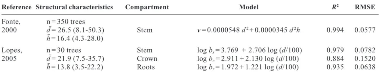
biomasses were calculated using models by Fonte (2000), and the allometric equations, for the stem, crown and roots components by Lopes (2005), respec-tively (see Table 1). Briefly, the volume equation was developed with a supporting dataset of 350 felled tre-es collected along the whole study area in reprtre-esenta- representa-tive stands. The system of allometric equations was ba-sed on data from 30 felled trees, collected in the county of Boticas in Tâmega’s Valley. The density of the sam-pled stands was 1062 trees ha–1with a mean age of 35 years (Lopes, 2005; Nunes et al., 2013). Stand volu-mes with bark (V, m3ha–1) were calculated as the sum of the volumes of the individual trees per plot and ex-panded for the hectare. Aboveground stand biomass (BABVG, Mgha–1) was def ined as the sum of stem and crown biomass of the living trees; total stand biomass (BTotal, Mgha–1) was defined as the sum of aboveground plus root biomass, expanded for the hectare.
Definition and calculation of BCEFs
The general definition of BCEF provided by IPCC (2006) is a multiplier with dimension (Mg m–3) that transform growing stock (m3) directly into above-ground biomass, or above-above-ground biomass growth or biomass removals (Mg):
Bi= BCEFi× V
BCEFs can be calculated for each stand (sampling plot), as the ratio of the biomass to the volume:
In this paper V refers to the stand volume with bark (m3ha–1) and B to the biomass (dry weight, Mg ha–1) of the i compartment: aboveground (stem and crown)
BCEFi= Bi V
Table 1. Equations used in the quantification of tree biomass and tree volume of maritime pine
Reference Structural characteristics Compartment Model R2 RMSE
Fonte, n = 350 trees
2000 d¯= 26.5 (8.1-50.3) Stem v = 0.0000548 d2+ 0.0000345 d2h 0.994 0.0577
h¯ = 16.4 (4.3-28.0)
Lopes, n = 30 trees Stem log bs= 3.769 + 2.706 log (d/100) 0.979 0.0782
2005 d¯= 21.9 (7.5-35.7) Crown log bc= 2.911 + 2.130 log (d/100) 0.884 0.1520
h¯ = 13.8 (3.5-22.2) Roots log br= 1.972 + 1.221 log (d/100) 0.935 0.0638
n: number of observations. d: diameter at breast height (cm). h: total height (m). d¯ and h¯ mean values of diameter and height, res-pectively; range values inside parenthesis. v: stem volume (m3) b: biomass (dry weight, kg) of the i compartment, in this case
and total (stem, crown and roots). Stand volume and biomass were evaluated as described before.
Datasets used in the hypothesis testing
Two distinct datasets were used in this study to pro-perly analyze the factors influencing the biomass con-version and expansion factors.
Time series data without recent thinning
For the time series study, the analysis was restric-ted to stands not subjecrestric-ted to thinning or not thinned at least in the 5 years period before the measurements were made. Available information refers to 41 perma-nent plots of undisturbed growth with a total of 105 observations (23 plots with 3 sets of measurements and 18 plots with 2 measurements).
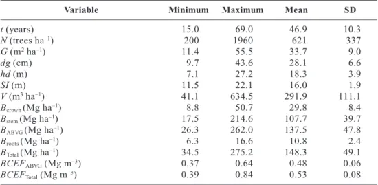
Characterization of the stand variables and of BCEFs is shown in Table 2.
Hereafter, the authors will refer to this data as time series dataset. These data comprise maritime pine stands at different stages of development as stated by the age variation, encompassing a wide range of den-sity, volume (V) and biomass (B). The site index va-lues show stands spans by lower quality (10≤ SI ≤ 14 m) and higher quality (18≤ SI≤ 22 m), with
predominan-ce on the average site-class quality (14≤ SI ≤ 18 m). The representation is according to the overall site qua-lity pattern observed in Tâmega’s Valley.
Cross sectional data in thinned stands
From the Data_Pinaster set, a total of 46 plots we-re selected to study the thinning effect. For this sub-set, information concerning tree and stand level varia-bles was recorded in detail. This allowed characterizing the diameter distribution before and after thinning, and the thinning practices. Characterization of stand variables and of biomass factors before and after thinning is shown in Table 3. The Table 4 summarizes the quantitative description of the thinning interven-tions made in the studied stands.
Model fitting and statistical analysis
Linear and nonlinear regression analyses were used to model the BCEFs against the studied stand bles and the thinning characteristics. Derived varia-bles, as well as interactions between variavaria-bles, were also considered in the data analysis procedures. Mul-ticolinearity was avoided by not allowing, in the same model regressors, variables with linear dependencies. The detection of undesirable dependencies was based
Table 2. Characterization of stand variables of the time series dataset (105 obs.)
Variable Minimum Maximum Mean SD
t (years) 15.0 69.0 46.9 10.3 N (trees ha–1) 200 1960 621 337 G (m2ha–1) 11.4 55.5 33.7 9.0 dg (cm) 9.7 43.6 28.1 6.6 hd (m) 7.1 27.2 18.3 3.9 SI (m) 11.5 22.1 16.0 1.9 V (m3ha–1) 41.1 634.5 291.9 111.1 Bcrown (Mg ha–1) 8.8 50.7 29.8 8.4 Bstem (Mg ha–1) 17.5 214.6 107.7 39.7 BABVG (Mg ha–1) 26.3 262.0 137.5 47.8 Broots (Mg ha–1) 6.3 16.6 10.8 2.4 BTotal (Mg ha–1) 34.5 275.2 148.3 49.1 BCEFABVG(Mg m–3) 0.37 0.64 0.48 0.06 BCEFTotal(Mg m–3) 0.39 0.84 0.53 0.08
t: Stand age. N: number of stems per hectare. G: basal area. dg: quadratic mean diameter. hd: do-minant height. SI: site index at 35 yr reference age. V: stem volume. B: biomass. BCEF: Biomass Conversion and Expansion Factor. AVBG refers to aboveground and Total refers to above and be-lowground biomass. SD refers to standard deviation.
on the coefficient of determination of the regression when Xiis regressed against the other explanatory va-riables (R2
i). The cut-off point of R2iwas set equal to 0.8, which corresponds to maintain the variance infla-tion actors, lower than 5 (Myers, 1990 and Neter et al., 1996). Candidate models were developed and residual analysis was carried out to examine the model appro-priateness for the assumptions of the error term.
The normality of the residuals of the models was analysed through the Shapiro-Wilk (Shapiro and Wilk, 1965) test. Whenever the Shapiro-Wilk test was indi-cative of departure of normality and the visual analy-sis pointed out to an increasing variance pattern of the
residuals, the Goldfeld-Quandt test for homocedasti-city (Goldfeld & Quandt, 1965) was applied. In case of corroboration of heteroscedasticity, weighed regres-sion analysis was performed.
The selection of the f inal model, from candidate models, was based on logical criteria and on the sum-mary statistics of f it criteria, such as the coeff icient of determination (R2) and the root mean square error (RMSE). For the nonlinear models, a statistic R2-like was used as a f it index. A 5% signif icance level was used throughout, unless stated otherwise. Sta-tistical analyses were made with and JMP 9.0® soft-ware.
Table 3. Characterization of the stand variables before and after thinning for the thinning dataset
Minimum Maximum Mean SD
Variable
Before After Before After Before After Before After Thin. Thin. Thin. Thin. Thin. Thin. Thin. Thin.
t (years) 18 18 52 52 38.17 38.17 7.28 7.28 N (trees ha–1) 280 220 4,060 3,260 1,229.13 913.00 838.44 608.81 G (m2 ha–1) 14.51 10.73 58.35 51.59 32.86 27.98 8.90 7.88 dg (cm) 10.34 11.29 33.87 36.64 20.71 21.79 5.26 5.09 hd (m) 10.50 10.50 23.02 23.02 15.27 15.27 2.77 2.77 SI (m) 9.70 9.70 19.49 19.49 14.84 14.84 2.47 2.47 V (m3ha–1) 102.11 74.41 477.28 435.41 236.16 200.82 89.17 75.75 Bcrown (Mg ha–1) 12.64 93.30 49.34 43.92 27.92 23.88 7.6 6.77 Bstem (Mg ha–1) 39.9 30.43 148.36 138.55 84.95 73.91 26.17 23.70 BABVG (Mg ha–1) 54.74 39.73 195.79 178.03 112.86 97.78 33.20 30.06 Broots (Mg ha–1) 4.96 3.76 24.53 21.20 13.56 11.13 4.69 3.83 BTotal (Mg ha-1) 59.70 43.48 220.32 198.35 126.43 108.92 35.59 32.19 BCEFABVG(Mg m–3) 0.39 0.41 0.59 0.60 0.49 0.50 0.05 0.05 BCEFTotal(Mg m–3) 0.43 0.43 0.66 0.68 0.55 0.56 0.06 0.06
For symbol definitions, please see Table 1.
Table 4. Summary statistics of thinning key criteria (46 obs.)
Thinning criteria Minimum Mean Median Maximum SD
Severity Nremoved(tree ha–1) 40 316 160 1,480 366 Gremoved(m2ha–1) 0.103 4.886 3.650 24.789 4.379 PN= Nremoved/ Nbefore 0.063 0.226 0.182 0.649 0.149 PG = Gremoved/Gbefore 0.003 0.145 0.113 0.445 0.107 Kind R = dgremoved/dgbefore 0.216 0.770 0.775 1.103 0.173
N: number of stems per hectare. G: basal area. dg: quadratic mean diameter. The Index removed re-fers to the removed stand and before rere-fers to the stand before thinning. PN: proportion of trees
re-moved. PG: proportion of basal area removed, with P being a fraction of unity. R: ratio between the
quadratic mean diameter of the thinned stand and the quadratic mean diameter of the stand before thinning. SD refers to standard deviation.
Results
Average values of BCEFABVG= 0.48 and BCEFTo-tal= 0.53 were found for the 105 sample plots (Table 2). According to the dispersion measures obtained for the conversion and expansion factors, it is confirmed that it is not appropriate to use an average value of BCEF for maritime pine. This applies to any of the compart-ments in the analysis. A slight increase of the factors following a thinning practice is noticeable, for above-ground component and whole tree (Table 3).
Changes in BCEFs with stands characteristics
and across time and development of prediction
models
A correlation analysis was performed to investiga-te the relationship between the BCEFs and the stand variables using the 105 observations of the time series data. The strongest linear association was found with hd, SI, V and t (|r| > 0.5), all in opposite trend. The va-riable selected as main regressor, for both the above-ground and total BCEFs models, was the dominant height. This variable combines simultaneously two pa-rameters of population: age and site index, hence it is
an interesting variable to describe the variation of the BCEFs while avoiding problems of multicolinearity.
Residual analysis of the fitted models allowed iden-tifying quadratic mean diameter as a supplementary variable to be included in the model.
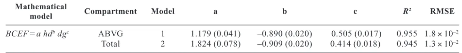
Scatterplots for the BCEFiagainst the explanatory variables hd and dg are shown in Fig. 1. The allome-tric model in the form BCEF = a hdbdgc, where a, b and c are the model parameters, was chosen as an ap-propriate functional form to model the relationships (Table 5). The estimation of the nonlinear models was made by applying the Gauss-Newton method at the nonlinear platform, of the JMP software. Analyses of the models were performed as described. In Table 5, Model 1 refers to the estimation of BCEF for the abo-veground component, whereas Model 2 refers to the estimation of BCEF for the aboveground and roots (to-tal) components.
The analysis of the residuals of the f itted models over the estimates of the BCEFs revealed a pattern of increasing variance. The presence of heteroscedasti-city was corroborated by the Goldfeld-Quandt test at a significance level of 0.05. This type of heteroscedas-ticity was modeled as a power function of dominant height, that is σi2=
σ2Xk, where X is hd. Estimation of k and fitting of the models using the weight functions
0.0 0.1 0.2 0.3 0.4 0.5 0.6 0.7 0.8 0.9 0 5 10 15 20 25 30 35 40 45 50 55 hd (m) 0.0 0.1 0.2 0.3 0.4 0.5 0.6 0.7 0.8 0.9 0 5 10 15 20 25 30 35 40 45 50 55 hd (m) 0.0 0.1 0.2 0.3 0.4 0.5 0.6 0.7 0.8 0.9 0 5 10 15 20 25 30 35 40 45 50 55 dg (cm) 0.0 0.1 0.2 0.3 0.4 0.5 0.6 0.7 0.8 0.9 0 5 10 15 20 25 30 35 40 45 50 55 dg (cm) BCEF ABVG BCEF ABVG BCEF total BCEF total BCEFABVG = 1.390 hd–0.368
BCEFABVG = 0.773 dg–0.142 BCEF
total = 1.394 dg–0.295
BCEFtotal = 2.317 hd–0.516
Figure 1. Measured Biomass Conversion and Expansion Factors (BCEFs) for the aboveground (ABVG) and Total compartments
versus stand dominant height (hd) and quadratic mean diameter (dg). (
•
plot value – time series data set). Line: fitted allometric equation in the model form BCEF = a Xb, where X is hd or dg.were according to the procedure proposed by Parresol (1999). The parameters (and the standard errors) of the nonlinear regression models estimated by the weigh-ted least squares regression method are shown in Ta-ble 5. Analysis of the residuals for the fitted models (done graphically and by the Goldfeld-Quandt test) confirmed the presence of a constant error variance. Also shown in Table 5 are the goodness of fit statistics coeff icient of determination and root mean square error for the proposed models.
According to the Shapiro-Wilk test results, the re-siduals of Model 1 follow a normal distribution (test statistic of 0.970, p-value = 0.137). Regarding Model 2, the test pointed towards a departure from normality (test statistic of 0.854; p-value < 0.0001). Visual analy-sis of the data (Fig. 1) and of the quantil-quantil plot (QQ) for the residuals were used to investigate the de-parture from normality. The QQ plot (graph not shown here) exposed a symmetrical distribution of the resi-duals, but with a heavy tail. The observations respon-sible for the results refer to the younger stands with lowest values of dominant height (hd) and quadratic mean diameter (dg). The observations are clearly vi-sible at the left side of the graphs plotted in Fig. 1. This deviation from normality does not affect the estimates of the parameters, which remain unbiased and consis-tent, thus it has no direct implications in the quality of the estimations. Hence, a further correction was deemed unnecessary.
Thinning practice effects in the BCEFs
and development of prediction models
A stepwise regression analysis and the “all possible models” analysis was performed as exploratory methods to investigate for the influence of stand characteristics and for the thinning variables descriptors on the varia-tion of the BCEFs values. The response variable was de-fined as the ratio between the value of the BCEF after thinning and its counterpart before thinning. The tested regressors for the stand characteristics were: stand age, number of trees per hectare, basal area, quadratic mean diameter, dominant height, site index. The thinning des-criptors tested were the number and basal area of trees removed (Nremovedand Gremoved, respectively), the propor-tion of trees removed (PN), the proporpropor-tion of basal area removed (PG), the ratio between the quadratic mean meter of the thinned stand and the quadratic mean dia-meter of the stand before thinning (dgremoved/dgbefore) and the ratio between the quadratic mean diameter of the stand after thinning and the quadratic mean diameter of the stand before thinning (dgafter/dgbefore).
From the set of the variables tested, the ratio dgafter/dgbefore presented a signif icant association (r > 0.7) with the variation of the BCEFs values for both compartments. For BCEFTotal, a high correlation value was also found with Nremoved(r = 0.772) and PN (r = 0.734). Tentative models were developed for the aboveground compartment and for the total. Table 6
Table 5. Parameters of the allometric models for BCEFs established using the time series data without thinning
Mathematical
Compartment Model a b c R2 RMSE
model
BCEF = a hdbdgc ABVG 1 1.179 (0.041) –0.890 (0.020) 0.505 (0.017) 0.955 1.8× 10⁻²
Total 2 1.824 (0.078) –0.909 (0.020) 0.414 (0.018) 0.945 1.3× 10⁻²
BCEF: Biomass Conversion and Expansion Factor (Mg m–3). hd: dominant height (m). dg: quadratic mean diameter (cm).
ABVG: aboveground. Total: aboveground and roots. The weighting function was 1/hdkwith k = –0.919 for the ABVG and k = –2.807
for total.
Table 6. Parameters of the allometric models for the ratio of BCEFs using the thinning dataset
Mathematical model Compartment Model a b c R2 RMSE BCEFafter/BCEFbefore= ABVG 3 0.948 (0.023) 0.019 (0.009) 0.321 (0.027) 0.765 1.1× 10⁻² a hdb(dg
after/dgbefore)c
BCEFafter/BCEFbefore= Total 4 1.037 (0.005) 0.015 (0.003) — 0.433 1.2× 10⁻² a PNb
BCEF: Biomass Conversion and Expansion Factor. The sub indexes after and before refer to after thinning and before thinning, respectively. hd: dominant height (m). dg: quadratic mean diameter (cm). PN: proportion of trees removed, with P being a fraction
presents the estimation results for the selected models, concerning the estimates of the parameters (standard errors) and the fit statistics. All coefficients are statis-tically significant.
The residual analysis has shown no problems con-cerning heteroscedasticity. According to the Shapiro-Wilk test results, the residuals are normally distributed (test value of 0.956, with p-value = 0.131 for Model 3; test value of 0.948, with p-value = 0.064 for Model 4).
Discussion
Models for estimation of BCEFs
The study showed that it is not appropriate to use average values of BCEF for obtaining biomass estima-tes for maritime pine, hence, neither is any constant value, regardless of the compartment under conside-ration (aboveground or total). Fig. 1 shows a great va-riation in BCEF values with the quadratic mean dia-meter and with the dominant height. BCEFs values also vary with age, quality of the location and stand volume. The decrease in the BCEFs with volume was reported by Brown (1997). The decrease in the BCEFs with tree size and age as the stands develops, tending to a constant value as the stands get older, are also in agreement with the findings reported by other authors (Lehtonen et al., 2004; Somogyi et al., 2006; Tobin & Nieuwenhuis, 2007; Faias, 2009; González-García et al., 2013 ).
Older stands and/or stands located in better sites tend to present lower values of factors. The decreases of BCEFs with respect to increasing values of domi-nant height were reported by other authors (Castedo-Dorado et al., 2012; Sanquetta et al., 2011; Faias, 2009; González-García et al., 2013). Sanquetta et al. (2011) and Faias (2009) also indicated a decreasing re-lationship between the conversion factors and biomass expansion and the tree diameter for stands of pine spe-cies.
The results can be analyzed based on the expecta-tion of achieving lower output biomass values for the same quantity of stem volume in younger stands, comparatively to an opposite trend that is expected to occur in older stands.
Two factors can interact and explain the phenome-non: (1) pattern of biomass allocation in the tree com-ponents (stem, branches, needles and roots), depen-ding on the stage of stand development and (2) the
growth rate. Sanquetta et al. (2011) explain this as-ymptotic decreasing behaviour due to the stabilization of growth rate and tree maturation. The authors provi-de full provi-details for the explanation of this trend. The re-ported pattern is also attributed to the existence of dis-tinct allometric coefficients along the developmental stage of stands with a higher relative allocation of bio-mass to the trunk component, as it progresses towards maturity. Results presented by Porté et al. (2002), re-garding the distribution of the total biomass by com-ponents for maritime pine stands of different ages, con-f irm this trend. According to the authors, the percentage of branches’ biomass relatively to the total biomass decreases significantly with age. In the study, the authors reported values of 49.3% at 5 years, com-pared to values of 13.2 and 11.4%, respectively, for stands of 26 and 32 years. Once the dominant height is a variable that simultaneously combines the age and quality of the station, it is expected that the dominant height indicator is even more relevant with BCEFs than age.
Evaluation of the influence of thinning
on the values of BCEFs
The separation of the maritime pine data in two sub-sets, according to the occurrence or not of thinning du-ring a minimum of a 5-year period, allowed investiga-ting whether or not this management practice produced an evident effect on the BCEFs variation. Results from the regression analysis pointed out that the application of BCEF factors to estimate forest biomass in stands subjected to thinning should explicitly account for the effect of thinning. Although this effect is expected to reduce as stand growths after thinning, during a period of non disturbance, better estimates of biomass can be obtained when thinning is accounted for. In general terms, the BCEF model for the above-ground compartment discloses a tendency to increase with dominant height. As this variable can be interpre-ted as a surrogate of age and site quality, greater va-riations are predicted for better sites and/or along stand development. The effect of the stage of stand develop-ment and the site quality was analyzed. Regarding the ratio of the diameters, characterizing the type of thinning, there is also a positive trend. With regard to the BCEF variable for the above and belowground components (BCEFTotal), there will be an increase of the values with an increasing proportion of trees
re-moved, that is, with the severity of the thinning. Re-sults are in accordance to the expected effects of a low to moderate selective thinning in stand growth after thinning. A short-term positive effect of thinning on tree growth, due to the increase of available space for growth, is well reported for the species (e.g. Luis & Guerra, 1999; Fonseca, 2004).
The proposed models estimate changes in the BCEFs after a thinning, depending on stand characte-ristics and on the thinning severity and type. The mo-dels (3) and (4) should be used in the 1-5 years period after the thinning is performed. After 5-years of non disturbance, models (1) and (2) can be securely applied.
Conclusions
For periods of undisturbed growth, the BCEF va-lues vary with stand age and with the quality of the sta-tion. These effects are accounted for into a surrogate variable, which is the stand dominant height. For a fi-xed value of the dominant height, variations of the BCEFs values are still observed. Results have shown that the differences are partially explained by the me-an size of the trees, described by the quadratic meme-an diameter, which is influenced by stand development and density. For increasing values of dominant height and of quadratic mean diameter, higher values of stand biomass are expected to occur.
The maritime pine stands are subjected to light thin-ning from below to moderate thinthin-ning. When thinthin-ning occurs, the thinning practice has proved to have an ob-vious effect in the variation of the BCEFs. With regard to the aboveground compartment, for a fixed value of dominant height, thinning type and thinning severity influence the variation of BCEF value. The effect is built-in the surrogate variable quadratic mean diame-ter ratio (dgafdiame-ter/dgbefore). The expected BCEF variation increases also with increasing values of the stand do-minant height. The variables which affect the variation of BCEF for the total compartments refer to the seve-rity of thinning, expressed in number of trees (PN).
The proposed BCEFs equations are simple but effective models that allow predicting the biomass of a stand from easier-to obtain stand characteristics such as dominant height and quadratic mean diameter. The-se variables are currently recorded in inventories. If a thinning is performed, the ratio models provide infor-mation of the expected change in the BCEFs,
depen-ding on the severity and type of the thinning. Further-more, the system of equations presented in this work easily conjugate with existing growth and yield mo-dels that solely provide information on stem volume, enlarging their outputs to biomass predictions. These prediction models should produce helpful biomass in-formation to support maritime pine management de-cisions for commercial uses (timber, energy supply and fiber) and environmental goods.
Acknowledgements
The authors would like to thank the commitment of Professor Carlos Pacheco Marques to obtain funding to support the installation and monitoring of perma-nent plots in the Valley Tâmega’s maritime pine (un-der PAMAF Project 4004 and Project Agro 372) which supported the database DataPinaster used in this study.
References
Baldwin VC, Peterson Jr KD, Clark III A, Ferguson RB, Strub MR, Bower DR, 2000. The effects of spacing and thinning on stand and tree characteristics of 38-year-old Loblolly Pine. For Ecol Manage 137: 91-102.
Brown S, 1997. Estimating biomass and biomass change of tropical forests: a Primer. FAO Forestry Paper. No. 134. Brown S, 2002. Measuring carbon in forests: current status
and future challenges. Environmental Pollution 116: 363-372.
Castedo-Dorado F, Gómez-García E, Diéguez-Aranda U, Ba-rrio-Anta M, Crescente-Campo F, 2012. Aboveground stand-level biomass estimation: a comparison of two me-thods for major forest species in northwest Spain. Ann For Sci 69: 735-746.
Eriksson E, 2006. Thinning operations and their impact on biomass production in stands of Norway spruce and Scots pine. Biomass and Bioenergy 30: 848-854.
Faias SMMP, 2009. Analysis of biomass expansion factors for the most important tree species in Portugal. M Sc the-sis. Instituto Superior de Agronomia, Lisboa, Portugal. Fonseca TF, 2004. Modelação do crescimento, mortalidade
e distribuição de diâmetro para povoamentos de pinheiro bravo no Vale do Tâmega. Ph D thesis. Universidade de Trás-os-Montes e Alto Douro,Vila Real, Portugal. Fonte CMM, 2000. Estimação de volume total e mercantil
em Pinus pinaster Ait. no Vale do Tâmega. Engenering Final Report. Universidade de Trás-os-Montes e Alto Dou-ro, Vila Real, Portugal.
Goldfeld SM, Quandt RE, 1965. Some tests for homosce-dasticity. Journal of the American Statistical Association 60: 539-547.
González-García M, Hevia A, Majada J, Barrio-Anta M, 2013. Above-ground biomass estimation at tree and stand level for short rotation plantations of Eucalyptus nitens (Deane & Maiden) Maiden in Northwest Spain. Bio-mass and Bioenergy 54: 147-157.
Hasenauer H, Burkhart HE, Amateis RL, 1997. Basal area development in thinned and unthinned loblolly pine plan-tations. Can J For Res 27: 265-271.
IPPC, 2006. Generic methodologies applicable to multiple land-use categories, Chapter 2. In: Guidelines for natio-nal greenhouse gas inventories. Agriculture, forestry and other land use, Vol 4 pp: 2.1-2.59.
Johnson WC, Sharpe DM, 1983. The ratio of total to mer-chantable forest biomass and its application to the global carbon budget. Can J For Res 13: 372-383.
Ketterings QM, Coe R, Noordwijk M, Ambagau Y, Palm CA, 2001. Reducing uncertainty in the use of allometric mass equations for predicting above-ground tree bio-mass in mixed secondary forests. For Ecol Manage 146: 199-209.
Lehtonen A, Mäkipää R, Muukkonen P, 2004. Biomass ex-pansion factors (BEFs) for Scots pine, Norway spruce and birch according to stand age for boreal forests. For Ecol Manage 188: 211-224.
Longuetaud F, Santenoise P, Mothe F, Kiessé TS, Rivoire M, Saint-André L, Ognouabi N, Deleuze C, 2013. Modeling volume expansion factors for temperate tree species in France. For Ecol Manage 292: 111-121.
Lopes DMM, 2005. Estimating net primary production in
Eucalyptus globulus and Pinus pinaster ecosystems in
Portugal. Ph D thesis. Kingston University, Kingston, UK. Luis JS, Fonseca TF, 2004. The allometric model in the stand density management of Pinus pinaster in Portugal. Ann For Sci 61: 807-814.
Luis JS, Guerra HP, 1999. Influence of alternative thinning regimes on Pinus pinaster Ait. stand dynamics in northern Portugal. Silva Lusitana 7: 11-21.
Marques CP, 1991. Evaluating site quality of even-aged ma-ritime pine stands in northern Portugal using direct and indirect methods. For Ecol Manage 41: 193-204
Myers RH, 1990. Classical and modern regression with applications, 2nded. PWS Publishers, USA. 488 pp.
Neter J, Kutner MH, Nachtsheim CJ, Wasserman W, 1996.
Applied linear regression models, 3rd ed. IRWIN,
USA.720 pp.
Nunes L, Lopes D, Rego FC, Stith TG, 2013. Aboveground biomass and net primary production of pine, oak and mi-xed pine-oak forests on the Vila Real district, Portugal. For Ecol Manage 305: 38-47.
Oliveira AC, Pereira JS, Correia AV, 2000. A silvicultura do pinheiro bravo. Centro Pinus, Porto, Portugal.
Pardé J, 1980. Forest biomass. Forestry Abstracts 41: 343-362.
Parresol BR, 1999. Assessing tree and stand biomass: a re-view with examples and critical comparisons. For Sci 45: 573-593.
Parresol BR, 2002. Biomass. In: Encyclopedia of environ-metrics (El-Shaarawi Abdel H, Piegorsch, Walter W). John Wiley & Sons, Ltd Chichester, UK. pp: 196-198. Páscoa F, Martins F, Salas R, João C, 2004.
Estabelecimen-to simultâneo de equações de biomassa para Pinheiro bra-vo. In: II Simpósio Iberoamericano sobre Gestión y Eco-nomia Forestal, Barcelona, Spain. pp: 18-20.
Picard N, Saint-André L, Henry M, 2012. Manual for buil-ding tree volume and biomass allometric equations: from field measurement to prediction. Food and Agricultural Organization of the United Nations, Rome, and Centre de Coopération Internationale en Recherche Agronomique pour le Développement, Montpellier. France. 215 pp. Porté A, Trichet P, Bert D, Loustau D, 2002. Allometric
re-lationship for branch and tree woody biomass of Mar-itime pine (Pinus pinaster Ait.). For Ecol Manage 158: 71-83.
Ruiz-Peinado R, Bravo-Oviedo A, López-Senespleda E, Montero G, Río M, 2013. Do thinnings influence biomass and soil carbon stocks in Mediterranean maritime pine-woods? Eur J For Res 132: 253-262.
Sanquetta CR, Corte APD, Silva F, 2011. Biomass expan-sion factor and root-to-shoot ratio for Pinus in Brazil. Car-bon Balance Manag 6: 6.
Shapiro SS, Wilk MB, 1965. An analysis of variance test for normality (complete samples). Biometrika 52: 591-611. Soares P, Tomé M, 2012. Biomass expansion factors
for Eucalyptus globulus stands in Portugal. For Syst 21: 141-152.
Somogyi Z, Cienciala E, Mäkipää R, Muukkonen P, Lehto-nen A, Weiss P, 2006. Indirect methods of large-scale fo-rest biomass estimation. Eur J For Res 126: 197-207. Telmo C, Lousada J, 2011. Heating values of wood pellets
from different species. Biomass and Bioenergy 35: 2634-2639.
Tobin J, Nieuwenhuis M, 2007. Biomass expansion factors for Sitka spruce (picea sitchensis (Bong.) (Carr.) in Irland. Eur J For Res 126: 189-196.
Viana H, Vega-Nieva DJ, Ortiz-Torres L, Lousada J, Aran-ha J, 2012. Fuel cAran-haracterization and biomass combus-tion properties of selected native woody shrub species from central Portugal and NW Spain. Fuel 102: 737-745.