Hargreaves and other reduced-set methods for calculating evapotranspiration

Hargreaves and Other Reduced-Set Methods

for Calculating Evapotranspiration

Shakib Shahidian

_{, Ricardo Serralheiro}

_{, João Serrano}

_,

José Teixeira

_{, Naim Haie}

_{and Francisco Santos}

1

_{University of Évora/ICAAM}

_{Instituto Superior de Agronomia}

_{Universidade do Minho}

Portugal

1. Introduction

Globally, irrigation is the main user of fresh water, and with the growing scarcity of this essential natural resource, it is becoming increasingly important to maximize efficiency of water usage. This implies proper management of irrigation and control of application depths in order to apply water effectively according to crop needs. Daily calculation of the Reference Potential Evapotranspiration (ETo) is an important tool in determining the water needs of different crops. The United Nations Food and Agriculture Organization (FAO) has adopted the Penman-Monteith method as a global standard for estimating ETo from four meteorological data (temperature, wind speed, radiation and relative humidity), with details presented in the Irrigation and Drainage Paper no. 56 (Allen et al., 1998), referred to hereafter as PM:













Rn – net radiation at crop surface [MJ m-2 day-1],

G – soil heat flux density [MJ m-2 _day-1_],

T – air temperature at 2 m height [ºC], u2 – wind speed at 2 m height [m s-1],

es – saturation vapor pressure [kPa],

ea – actual vapor pressure [kPa],

es-ea – saturation vapor pressure deficit [kPa],

∆ – slope vapor pressure curve [kPa ºC-1_],

γ – psychrometric constant [kPa ºC-1_],

The PM model uses a hypothetical green grass reference surface that is actively growing and is adequately watered with an assumed height of 0.12m, with a surface resistance of 70s m-1

and an albedo of 0.23 (Allen et al., 1998) which closely resemble evapotranspiration from an extensive surface of green grass cover of uniform height, completely shading the ground

and with no water shortage. This methodology is generally considered as the most reliable, in a wide range of climates and locations, because it is based on physical principles and considers the main climatic factors, which affect evapotranspiration.

Need for reduced-set methods

The main limitation to generalized application of this methodology in irrigation practice is the time and cost involved in daily acquisition and processing of the necessary meteorological data. Additionally, the number of meteorological stations where all these parameters are observed is limited, in many areas of the globe. The number of stations where reliable data for these parameters exist is an even smaller subset.

There are also concerns about the accuracy of the observed meteorological parameters (Droogers and Allen, 2002), since the actual instruments, specifically pyranometers (solar radiation) and hygrometers (relative humidity), are often subject to stability errors. It is common to see a drift, of as much as 10 percent, in pyranometers (Samani, 2000, 1998). Henggeler et al. (1996) have observed that hygrometers loose about 1 percent in accuracy per installed month. There are also issues related to the proper irrigation and maintenance of the reference grass, at the weather stations. Jensen et al. (1997) observed that many weather stations are often not irrigated or inadequately irrigated, during the summer months, and thus the use of relative humidity and air temperature from these stations could introduce a bias in the computed values for ETo. Additionally, they observed that the measured values of solar radiation, Rs, are not always reliable or available and that wind data are quite site specific, unavailable, or of questionable reliability. Thus, they recommend the use of ETo equations that require fewer variables. These authors compared various methods, including FAO Penman Monteith, PM, and Hargreaves and Samani, HS, with lysimeter data and noted r2 _{values of 0.94-0.97, with monthly SEE values of 0.30-0.34mm.}

Based on these data they concluded that the differences in ETo values, calculated by the different methods, are minor when compared with the uncertainties in estimating actual crop evapotranspiration from ETo. Additionally, these equations can be more easily used in adaptive or smart irrigation controllers that adjust the application depth according to the daily ETo demand (Shahidian et al., 2009).

This has created interest and has encouraged development of practical methods, based on a single or a reduced number of weather parameters for computing ETo. These models are usually classified according to the weather parameters that play the dominant role in the model. Generally these classifications include the temperature-based models such as Thornthwaite (1948); Blaney-Criddle (1950) and Hargreaves and Samani (1982); The radiation models which are based on solar radiation, such as Priestly-Taylor (1972) and Makkink (1957); and the combination models which are based on the energy balance and mass transfer principles and include the Penman (1948), modified Penman (Doorenbos and Pruitt, 1977) and FAO PM (Allen et al., 1998).

Objectives and methods

The objective of this chapter is to review the underlying principles and the genesis of these methodologies and provide some insight into their applicability in various climates and regions. To obtain a global view of the applicability of the reduced-set equations, each equation is presented together with a review of the published studies on its regional calibration as well as its application under different climates.

The main approach for evaluation and calibration of the reduced-set equations has been to use the PM methodology or lysimeter measurements as the benchmark for assessing their performance. Usually a linear regression equation, established with PM ETo values or lysimeter readings plotted as the dependent variable and values from the reduced-set equation plotted as the independent variable. The intercept, a, and calibration slope, b, of the best fit regression line, are then used as regional calibration coefficients:

( )

o o

ET PM a b ET Equation  (2)

The quality of the fit between the two methodologies is usually presented in terms of the coefficient of determination, r2_{, which is the ratio of the explained variance to the total}

variance or through the Root Mean Square Error, RMSE:





1

1 n

yi PM

i

RMSE ETo ETo

n _





and the mean Bias error:





1

1 n

yi PM

i

MBE ETo ETo

n _





where n is the number of estimates and ETo yi is the estimated values from the reduced-set

equation.

2. Temperature based equations

Temperature is probably the easiest, most widely available and most reliable climate parameter. The assumption that temperature is an indicator of the evaporative power of the atmosphere is the basis for temperature-based methods, such as the Hargreaves-Samani. These methods are useful when there are no data on the other meteorological parameters. However, some authors (McKenny and Rosenberg, 1993, Jabloun and Sahli, 2007) consider that the obtained estimates are generally less reliable than those which also take into account other climatic factors.

Mohan and Araumugam (1995) and Nandagiri and Kovoor (2006) carried out a multivariate analysis of the importance of various meteorological parameters in evapotranspiration. They concluded that temperature related variables are the most crucial required inputs for obtaining ETo estimates, comparable to those from the PM method across all types of climates. However, while wind speed is considered to be an important variable in arid climate, the number of sunshine hours is considered to be the more dominant variable in sub-humid and humid climates.

2.1 The Hargreaves- Samani methodology

Hargreaves, using grass evapotranspiration data from a precision lysimeter and weather data from Davis, California, over a period of eight years, observed, through regressions, that for five-day time steps, 94% of the variance in measured ET can be explained through average temperature and global solar radiation, Rs. As a result, in 1975, he published an equation for predicting ETo based only on these two parameters:

0.0135 ( 17.8)

o s

ET  R T (5)

where Rs is in units of water evaporation, in mm day-1_{, and T in ºC. Subsequent attempts to}

use wind velocity, U2, and relative humidity, RH, to improve the results were not

encouraging so these parameters have been left out (Hargreaves and Allen, 2003).

The clearness index, or the fraction of the extraterrestrial radiation that actually passes through the clouds and reaches the earth’s surface, is the main energy source for evapotranspiration, and later studies by Hargreaves and Samani (1982) show that it can be estimated by the difference between the maximum, Tmax, and the minimum, Tmin daily

temperatures. Under clear skies the atmosphere is transparent to incoming solar radiation so the Tmax is high, while night temperatures are low due to the outgoing longwave radiation

(Allen et al., 1998). On the other hand, under cloudy conditions, Tmax is lower, since part of

the incoming solar radiation never reaches the earth, while night temperatures are relatively higher, as the clouds limit heat loss by outgoing longwave radiation. Based on this principle, Hargreaves and Samani (1982) recommended a simple equation to estimate solar radiation using the temperature difference, T:

0.5 max min ( ) s T a R _{K T T} R   (6)

where Ra is the extraterrestial radiation in mm day-1_{, and can be obtained from tables}

(Samani, 2000) or calculated (Allen et al., 1998). The empirical coefficient, KT was initially

fixed at 0.17 for Salt Lake City and other semi-arid regions, and later Hargreaves (1994) recommended the use of 0.162 for interior regions where land mass dominates, and 0.190 for coastal regions, where air masses are influenced by a nearby water body. It can be assumed that this equation accounts for the effect of cloudiness and humidity on the solar radiation at a location (Samani, 2000). The clearness index (Rs/Ra) ranges from 0.75 on a clear day to 0.25 on a day with dense clouds.

Based on equations (5) and (6), Hargreaves and Samani (1985) developed a simplified equation requiring only temperature, day of year and latitude for calculating ETo:

0.5 min

0.0135 ( 17.78)( )

o T mzx a

ET  K T T T R (7)

Since KT usually assumes the value of 0.17, sometimes the 0.0135 KT coefficient is replaced

by 0.0023. The equation can also be used with Ra in MJ m-2 _day-1_{, by multiplying the right}

hand side by 0.408.

This method (designated as HS in this chapter) has produced good results, because at least 80 percent of ETo can be explained by temperature and solar radiation (Jensen, 1985) and T is related to humidity and cloudiness (Samani and Pessarakli, 1986). Thus, although this equation only needs a daily measurement of maximum and minimum temperatures, and is presented here as a temperature-based method, it effectively incorporates measurement of radiation, albeit indirectly. As will be seen later, the ability of the methodology to account for both temperature and radiation provides it with great resilience in diverse climates around the world.

Sepashkhah and Razzaghi (2009) used lysimeters to compare the Thornthwaithe and the HS in semi-arid regions of Iran and concluded that a calibrated HS method was the most accurate method. Jensen et al.(1997) compared this and other ETo calculation methods and concluded that the differences in ETo values computed by the different methods are not larger than those introduced as a result of measuring and recording weather variables or the uncertainties

associated with estimating crop evapotranspiration from ETo. López-Urrea et al. (2006) compared seven ETo equations in arid southern Spain with Lysimeter data, and observed daily RMSE values between 0.67 for FAO PM and 2.39 for FAO Blaney-Criddle. They also observed that the Hargreaves equation was the second best after PM, with an RMSE of only 0.88.

Since the HS method was originally calibrated for the semi-arid conditions of California, and does not explicitly account for relative humidity, it has been observed that it can overestimate ETo in humid regions such as Southeastern US (Lu et al. 2005), North Carolina (Amatya et al. 1995), or Serbia (Trajkovic, 2007).

In Brasil, Reis et al. (2007) studied three regions of the Espírito Santo State: The north with a moderately humid climate, the south with a sub-humid climate, and the mountains with a humid climate (Table 1). The HS equation overestimated ETo in all three regions by as much as 32%, but the performance of the HS equation improved progressively as the climate became drier. Only further south, at a latitude of 24º S, and in a warm temperate climate did HS provide good agreement with PM, though still with a small overestimation. Borges and Mendiondo (2007) obtained an r2 _{of 0.997 for HS when compared to PM, when using a}

calibrated  of 0.0022 (Sept-April) and 0.0020 for the rest of the year.

On the other hand, in dry regions such as Mahshad, Iran and Jodhpur, India, the HS equation tends to underestimate ETo by as much as 24% (Rahimkoob, 2008; Nandagiri and Kovoor, 2006). Rahimkoob (2008) studied the ETo estimates obtained from the HS equation in the very dry south of Iran. His data indicate that the HS equation fails to calculate ETo values above 9 mm day-1_{, even when the PM reaches values of more than 13 mm day}-1 _{(Fig. 1).}

Wind removes saturated air from the boundary layer and thus increases evapotranspiration (Brutsaert, 1991). Since most of the reduced-set equations do not explicitly account for wind speed, it is natural for the calibration slope to be influenced by this parameter. Itensifu et al. (2003) carried out a major study using weather data from 49 diverse sites in the United States. They obtained ratios ranging from 0.805 to 1.242 between HS and PM and concluded that the HS equation has difficulty in accounting for the effects of high winds and high vapor pressure deficits, typical of the Great Plains region. They also observed that the HS equation tends to overestimate ETo when mean daily ETo is relatively low, as in most sites in the eastern region of the US, and to underestimate when ETo is relatively high, as in the lower Midwest of the US. As will be seen later, this seems to be a common issue with most of the reduced set evapotranspiration equations (see section 4.3, Fig. 7).

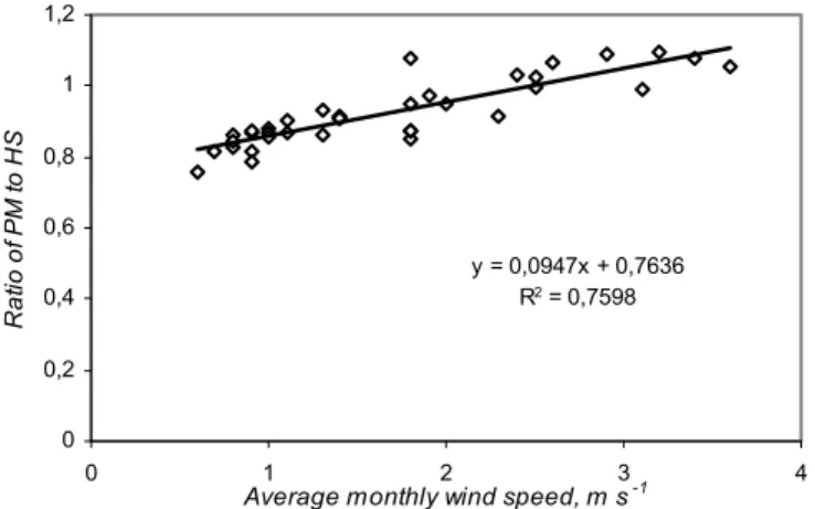
For the Mkoji sub-catchment of the Great Ruaha River in Tanzania, Igbadun et al. (2006) calculated the monthly ETo values of three very distinct areas of the catchment: the humid Upper Mkoji with an altitude of 1700m, the middle Mkoji with an average altitude of 1100 m, and the semi-arid lower Mkoji with an altitude of 900m. Their data indicate a strong relation between the monthly average wind speed and the performance of the HS equation as measured by the slope of the calibration equation (PM/HS ratio). Although the three areas have distinct climates, the HS equation clearly underestimated ETo for wind speed values below 2-2.3 ms-1_{, and overestimated it for higher wind speed values (Fig. 2).}

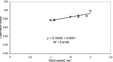
Trajkovic, et al. (2005) studied the HS equation in seven locations in continental Europe with different altitudes (42-433m) with RH ranging from 55 to 71%, representative of the distinct climates of Serbia. Their data show that despite the different altitudes and climatic conditions, wind speed was the major determinant for the calibration of the HS equation (Fig. 3). The results from these works indicate that wind is the main factor affecting the calibration of the HS equation and that the equation should be calibrated in areas with very high or low wind speeds.

0 2 4 6 8 10 12 14 0 2 4 6 8 10 12 14

Hargreaves Samani ETo, mm day-1

F A O P e n m an M o nt eit h , E T o, m m day -1

Fig. 1. Relation between ETo calculated with the HS equation and the PM for the dry conditions of Abadan, Iran. The Hargreaves Samani equation fails to calculate ETo values above 9 mm day-1 _{(data kindly provided by Rahimkoob)}

y = 0,0947x + 0,7636 R2 _{= 0,7598} 0 0,2 0,4 0,6 0,8 1 1,2 0 1 2 3 4

Average monthly wind speed, m s-1

R a tio o f P M to H S

Fig. 2. Correlation between average wind speed and the calibration slope in distinct climates of the Great Ruana River in Tanzania (based on the original data from Igbadun et al. 2006). Jabloun and Sahli (2008) studied eight stations in the semi-arid Tunisia and concluded that in inland stations, HS tends to overestimate ETo due to high T values. In the coastal station of Tunis, HS underestimated ETo values, which they attributed to an underestimation of Rs. Various attempts have been made to improve the accuracy of the HS equation through incorporation of additional measured parameters, such as rainfall (Droogers and Allen, 2002) and altitude (Allen, 1995). These methodologies have had limited global application, probably because ETo is influenced by a combination of different parameters, and although in a certain region there appears to be a good correlation between the calibration slope and a certain parameter, this might not be so in a different climate.

The alternative is to use regional calibration, in which, based on the climatic characteristics of the region, the ETo calculated by the HS equation is adjusted to account for the combined

effect of the dominant climate parameters, and thus accuracy of the equations is improved (Teixeira et al., 2008). Table 1 presents a compilation of most of the published studies on the regional calibration of the HS equation. This compilation contains 33 published works covering 21 countries with all types of climatic conditions according to the Koppen classification. Whenever various stations from a similar climate were studied, only parameters from one representative station are presented. In some studies, HS and PM were calibrated against a third methodology (such as Pan A) and thus no direct calibration parameters for the PM/HS regression were provided. In these cases, a linear regression was obtained by plotting the PM calibration equation as the dependent variable and the HS calibration equation as the independent variable. The parameters of the resulting regression equation are then presented as the PM-HS calibration parameters.

In order to contextualize the information and allow for extension of the results to other regions with a similar climate, the locations are grouped according to Koppen climate classification. These calibration coefficients can be used in the area where they were obtained or can be extrapolated for areas with similar conditions where no actual calibration has been carried out yet.

y = 0.1649x + 0.6001 R2 _{= 0.8195} 0.00 0.20 0.40 0.60 0.80 1.00 1.20 0 0.5 1 1.5 2 2.5 Wind speed, ms-1 C al ibr at ion s lope

Fig. 3. Correlation between wind speed and the calibration slope for seven different locations in Serbia, representing the diverse local climates (original data from Trajkovic, 2005).

2.2 The Thornthwaite method

Thornthwaite (1948) devised a methodology to estimate ETo for short vegetation with an adequate water supply in certain parts of the USA. The procedure uses the mean air temperature and number of hours of daylight, and is thus classified as a temperature based method. Monthly ETo can be estimated according to Thornthwaite (1948) by the following equation:

 



0 0 N₁₂ dm₃₀

C oun tr y S tat io n lat itud e A lti tu de K op pe n R ai nf al l R H U 2 R 2 R MS E S ou rc e m m cl assi ficat ion m m % ms -1 in te rc ep t slo pe ab Ar id De se rt Ch in a, N W Sh an da n He ih e R . 38 º9 0' N 148 3 B W k 250 40 1. 98 0. 54 31 1. 14 8 Z ha o e t a l. 2005 Ch in a, N W Mi nl e 38º8 0' N 227 1 B W k 100 -0 .3 2 1. 06 5 Zh ao e t a l. 2 005 US Aq ui la 33 º5 6' N 655 B W h 195 35. 3 3. 2 0. 03 78 1. 3155 A le xa nd ris , 20 06 St ep pe Indi a Jo dhp ur 26 º1 8' N 224 BS h 402 38. 9 2. 1 -0 .3 82 7 1. 1924 N an da gi ri a nd K ov oor , 20 06 Indi a H ey da raba d 17º3 2' N 545 BS h 820 65. 6 2. 8 -1 .9 7 1. 48 N an da gi ri a nd K ov oor , 20 06 S yr ia T el Ha dy a 36º0 1' N 293 BS h 231 57. 4 2. 82 1. 04 0. 91 S tock le, 2 00 4 Ir an Sh ira z 30º 07 'N 16 50 BS h 306 36. 4 2. 49 0. 41 0. 82 R az za gh i an d S ep ahsk ah, 20 09 Ir an Sh ira z 30 º0 7' N 165 0 B S h 30 5. 6 36 .4 2.4 9 1. 13 S epa sh ka h an d Ra zz aghi , 20 09 Méxi co Prog re so (Y ucat án ) 21º1 7' N 2 BS h 511 -0 .2 6 1. 01 2 0. 78 B aut is ta e t a l 2 009 D ry summ er S pa in D ar oca (NE S pa in) 41 º0 7' N 779 B sk 364 66. 5 1. 08 -0. 20 3 0. 93 M ár tine z-C ob a ndTejero-J us te, 20 04 S pa in Z arago za ( N E S pai n) 41 º4 3' N 225 B sk 353 73. 7 2. 43 -0. 01 2 0. 99 M ár tine z-C ob a ndTejero-J us te, 20 04 S pa in Co rd ob a, in la nd 37 º5 2' N 117 B sk 696 63. 3 1. 6 1. 06 G av ilá n et a l, 20 08 B ol iv ia Pa ta cam ay a a nd O ru ro 17º 15'S 374 9 B sk 375 57. 4 1. 2 0. 86 22 0. 6422 G arc ia e t a l 2 004 S pa in A lb acet e 39º1 4' N 695 B sk 283 68. 7 1. 08 0. 34 * 1.1 4* Lo pé z-U rra et al 20 05 S pa in C or do ba , i nl and 37 º5 1' N 110 B sk 696 63. 3 1. 6 -1 .4 9 1.3 B er enge na a nd G av ila n, 20 05 T anz an ia Lo w er M koj i 7º 80 ' 90 0 B sh 52 0 -0 .0 02 7 0.90 92 Ig ba du n et al Mesoth ermal M ed ite rr an ean S pa in M al ag a ( A nd al uci a) C oa st 36º4 0' N 7 C sa 531 68. 1 1. 9 0. 96 2 V anderl in de n et al ., 200 4 Sp ain S evilla ( A nd al uc ia) in te rio r 37 º1 25 ' N 31 C sa 473 67. 8 0. 93 1. 16 5 V anderl in de n et al ., 200 4 S pa in La Mo jone ra , coa st 37º4 5' N 142 C sa 272 62. 3 1. 9 1. 27 G av ilá n et a l, 20 08 Po rt ug al, S E vor a 38 º5 5' N 24 6 Cs a 627 63. 3 4. 3 0. 86 6 S an to s and Mai a, 20 07 US Da vi s 38º3 2' N 18 .3 C sa 458 63. 3 2. 62 -0. 84 4 1. 24 5 A le xa nd ris , 20 06 Po rt ug al E lvas 38 º60 ' N 20 2 Cs a 508 58. 2 1. 97 -0 .0 8 1.0 4 T eix eir a et al. 2 00 8 S pa in N ie bl a (An da luci a) 37º2 1' N 52 C sa 702 65. 3 1. 3 1. 03 5 0. 93 G av ilá n et a l., 20 08 S pa in V ej er Fron te ra (A nd al uci a) 36 º 17 ' N 24 C sa 571 69. 4 2. 9 1. 40 4 G av ilá n e t a l., 20 08 G reece A th ens 38 º2 3' N 100 C sa 371 61. 8 1. 87 0. 264 0. 78 1 A le xa nd ris, 20 06 US A P rosser , W A 46 º1 5' N 380 C sb 994 69 .7 1.6 2 1.0 2 0.9 8 S to ck le , 20 04 Sp ain Lle ida 41 º42 ' N 22 1 Cs b 601 68. 8 0. 97 1. 1 0.9 5 S to ck le , 20 04 Dry w int er T an zani a M iddl e Mk oj i 8º3 0' 10 70 Cw a 800 -0 .4 0. 95 5 Igb ad un e t a l, 20 06 B ra si l Do ur ad as , Mat o G . S ul 22º 16'S 452 Cw a 16 03 73. 8 1. 74 1.7 3 0. 67 0. 7 Fi et z, 20 04 B ra si l S. Man tique ira , MG 15 00 Cw b 21 50 0. 153 1. 16 P er ei ra et al . 20 09 fu lly hu mid N eth er la nd s H aa rw eg 51 º5 8' N 9 C fb 778 87. 3 2. 41 1. 02 0. 91 S tock le, 2 00 4 US Lou is ia na , i nl and 31 º N low land Cfa 15 00 92 0. 82 -0 .28 1. 05 Fo nt en ot , 2 00 4 US Lou si san a, c oast al 29º N low land Cfa 15 00 88. 7 0. 6 -0 .1 7 0. 87 F on te no t, 20 04 US No rt h Ca ro lin a, P ly m ou th 35 º52 ' 6 C fa 12 99 80. 2 4. 9 0. 03 0.8 3 1. 23 Am at ya et al. 1 99 5 Br as il P alo tin a, Par aná 24 º1 8' S 31 0 C fa 170 0 73. 8 1. 74 -1 08 1 S yp er re ck , 2 00 6 B ra si l Ja cu pi ra ng a r iv er, S P 24 º29'S 52 C fa 18 79 91. 5 0. 97 -0. 36 5 1. 04 2 B or ge s a nd Me nd iond o, 20 07 V al ues in g re y ar e a nnu al av er ag es obt ai ne d from Cl im w at da ta b ase. W hen cal ib ra tio n pa ra m ete rs of th e HS v sFA O P M w ere no t di rect ly p rov id ed , lin ea r r egr es si on eq uat io ns w ere est ab lis hed w ith F A O -5 6 P M da ily E T 0 e st im at es as th e de pen de nt va riab le an d da ily E T 0 va lu es e st im at ed by H S as an i nd ep en den t v ari ab le . T he pa ra m et ers of th e r egress io n eq ua tio n w er e th en p resen ted a s t he cal ib ra tio n p ara m ete rs . Re gr es si on ad ju stm ent

Table 1. Regional calibration for the Hargreaves Samani equation compiled from published works C ou n try S ta tio n lat itu d e A ltit u d e C lass ific at ion R ain fall R H U 2 R 2 R MS E S ou rce m m Ko ppe n m m % m s -1 in te rc ep t slop e ab M ic rothe rm al F u lly h u m id Se rb ia K ra guj ev ac 4 4 º0 0 ' N 1 90 D fa 7 5 % 1 0 .7 8 0 .4 51 T ra jk ov ic , 20 05 Se rb ia B el g ra d e 4 4 º4 5 ' N 1 32 D fa 684 69 % 1 .7 0 .99 T ra jk ov ic , 20 05 C ro ., Se r. Bo s. Z agr eb , S ar aj ev o, e tc . 42 .6 - 46 .1 42 -6 30 D fb 6 8-76 1. 0-1. 9 0 .4 24 (3 ) T ra jko vi c, 2 0 0 7 C ana da So u th er n On ta rio , D ru m bo 43 º1 6' N 3 1 0 D fb 7 9% 1 .5 0 .7 4 0 .7 0. 70 4 S en te lh as e t al . 2 0 1 0 C an ad a S out he rn O n ta rio , H ar ro w 4 2º 12 ' N 1 90 D fb 7 3 % 2. 2 0 .9 4 0 .6 4 0 .7 04 S ent el h as e t al . 20 10 Dr y wi n te r C h in a T ib et e pl at ea Y u shu 3 3 º0 6 ' N 3 6 8 1 D w b 2 0 0 4 5 .4 0. 83 0. 34 7 0 .8 83 0 .91 0. 62 2 Y e e t a l. 20 09 Po la r Bul g ar ia T ra ce p la in, Pl ov di v 4 2º 25' N 1 60 ET 492 1 .11 P opo va e t al , 20 06 Sw itz er la n d C h an g in s 4 6º 24' N 4 16 ET 904 7 3 2. 5 -0. 31 1 .12 0. 9 9 X u a n d Si ng h, 2 0 0 2 T rop ical W inte r dr y M é xi co M é rid a ( Y uc at án ) 2 0º 56 ' N 1 5 A w 1 1 .74 0. 17 54 1. 02 1 0 .7 8 B au tis ta e t a l 20 09 T an za n ia U p p er M ko ji 9 º0 0 ' 17 00 A w 1 0 7 0 7 7 .5 1. 23 0. 00 6 0 .9 87 Ig ba du n et a l In di a K ha ra g p u r Aw -2 .6 4 1 .5 6 1 K as h ya p a n d Pa nd a, 2 0 0 1 In di a B an g al or e 1 3 º0 0 ' N 9 21 Aw 940 6 6 1. 9 -0 .106 3 1 .0 244 N and ag iri a n d Ko vo or , 20 06 N ige ria A be ok u ta 7 º1 0 ' S 6 2 A w 1 5 0 6 9 2 2 .1 2 -1. 41 0. 93 8 A de b oy e, 20 09 N ige ria A be ok u ta 7 º1 0 ' S 6 3 A w 1 5 0 6 9 2 2 .1 2 0 .0 02 5 (1 ) 16 .8 (2 ) A d eb oy e, 2 0 0 9 Br as il G oi âni a, G O 1 6 º2 8 ' S 8 23 Aw 17 85 87 .9 0 .8 2 0. 69 23 0. 3 811 0. 4 7 O liv ei ra e t al . 2 005 B ras il S oore ta m a (S ou th E sp irit o S an to 1 9 º22' S 7 5 A m 7 5 .9 3 .3 4 -2. 62 1. 57 2 R ei s e t a l, 2 0 0 7 Sum m er dr y Br as il C am p in a G ra n d e 7º 14 'S 5 5 0 A s' 700 8 0 1 .3 8 -0 .4 88 0. 89 3 H en riqu e, 200 6 F u lly h u m id Br as il N or th R io de J ane iro 2 1 °19'S 13 A f 1 1 7 2 .9 73 .1 0. 3 -0. 76 1 M en d on ça e t a l 20 03 P h ilip in es L os B an os 1 4 º1 3 ' N 4 1 A f 1 9 8 7 8 3 .3 1 .3 5 0 .9 6 0 .6 5 S to ck le, 2 0 0 4 * co m p ar ed w ith ly si m ete r v alue s V alu es in g re y are a n n u al av erag es o b ta in ed fr om C lim w at d at a b as e. (1 ) ( 2 ) ( 3 ) R espe ct iv el y, t h e K ’T , d a n d e o f r eg io n al ly c al ib ra te d H S e q u at io n , ac co rd in g to Eq u atio n 7 in th e te xt . W h en c al ib ra tio n pa ra m et er s o f t h e H S v sF A O PM w er e no t di re ct ly pr ov id ed , l in ea r r egr es si on e q ua tio n s w er e e sta bl is h ed w ith F A O -56 PM d ai ly ET 0 e sti m ate s a s th e de pe n d en t v ar ia b le a n d da ily E T 0 v al u es es tim at ed b y H S a s an in de p en d en t v ar ia b le . T h e p ar am ete rs o f th e re g re ssi on e q ua tio n w er e t h en pr es en te d as th e ca lib ra tio n pa ram et ers . R eg res si on a d ju st m en t

Where N is the maximum number of sunny hours as a function of the month and latitude and dm is the number of days per month. ETosc is the gross evapotranspiration (without

corrections) and can be calculated as:

0 16 10Ta

Et sc _{ I} _a (9)

where Ta is the mean daily temperature (°C), a is an exponent as a function of the annual

index: a = 0.49239 + 1792 × 10-5 _{I - 771 × 10} -7 _I2 _{+ 675 × 10}-9 _I3_{; and I is the annual heat index}

obtained form the monthly heat indecies:

12 1 1.514 5 m m T I        



Bautista et al. (2009) found that the precision of the Thorntwaite methodology improved during the winter months in Mexico. Garcia et al. (2004) observed that under the dry and arid conditions of the Bolivian highlands the Thornthwaite equation strongly underestimates ETo because the equation does not consider the saturation deficit of the air (Stanhill, 1961; Pruitt, 1964; Pruitt and Doorenbos, 1977). Additionally, at high altitudes, the Thornthwaite equation also underestimates the effect of radiation, because the equation is calibrated for temperate low altitude climates. Studies in Brazil have shown that the underestimation of ETo produced by temperature-based equations under arid conditions, may be reduced by using the daily thermal amplitude instead of the mean temperature (Paes de Camargo, 2000) as in the case of the Hargreaves–Samani equation.

Gonzalez et al. (2009) studied the Thorthwaite method in the Bolivian Amazon. They observed that the Thornthwaite method underestimates evapotranspiration at all the three stations studied. This is expected, considering that normally this method leads to underestimations in humid areas (Jensen et al., 1990).

2.3 Blaney-Criddle method

The FAO Temperature Methodology recommended by Doorenbos and Pruitt (1977) is based on the Blaney-Criddle method (Blaney and Criddle, 1950), introducing a correction factor based on estimates of humidity, sunshine and wind.





o

ET    _p T _{ (11)}

where  and β are calibration parameters and p is the mean annual percentage of daytime hours. Values for  can be calculated using the daily RHmin and n/N as follows:

min 0.043RH n 1.41 N  _ _   (12)





For windy South Nebraska, Irmak et al. (2008) compared 12 different ET methodologies and found that the Blaney–Criddle method was the best temperature method and it had an RMSE value (0.64 mm d−1_{) which was similar to some of the combination methods. The}

obtained estimates were good and were within 3% of the ASCE-PM ETo with a high r2 _of

0.94. The estimates were consistent with no large under or over estimations for the majority of the dataset. They attributed this to the fact that, unlike most of the other temperature methods, this method takes into account humidity and wind speed in addition to air temperature.

Lee et al. (2004) compared various ETo calculation methods in the West Coast of Malaysia and concluded that the Blaney-Criddle method was the best, among the reduced-set equations, for estimating ET in the region. They also observed that HS gave the highest estimates followed by the Priestly-Taylor equation. Similarly, in the humid Goiânia region of Brazil, Oliveira et al. (2005) observed that the Blaney-Criddle method produced the best results, next to the full PM equation.

Various studies indicate that the Blaney-Criddle equation might show some bias under arid conditions. For semi-arid conditions of Iran, Dehghani Sanij et al. (2004) found the Blaney-Criddle and the Makkink method to overestimate ETo during the growing season. Lopéz-Urrea et al. (2006) compared seven different methods for calculating ETo in the semiarid regions of Spain and observed that the Blaney-Criddle method significantly over-estimated average daily ETo.

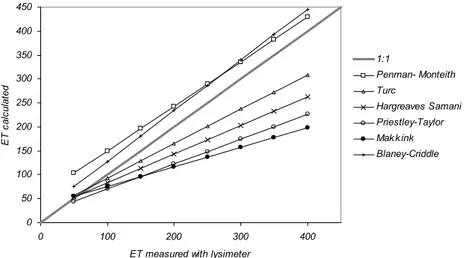
For arid conditions of Iran, Fard et al. (2009) compared nine different methodologies with lysimeter data and observed that the Turc and the Blaney-Criddle methods showed very close agreement with the lysimeter data, while PM showed moderate agreement with the lysimeter data. The other methods showed bias, systematically over estimating the lysimeter data (Fig. 4).

Although recognizing the historical value of the Blaney-Criddle method and its validity, the FAO Expert Commission on Revision of FAO Methodologies for Crop Water Requirements (Smith et al. 1992) did not recommend the method further, in view of difficulties in estimating humidity, sunshine and wind parameters in remote areas. Nevertheless, they emphasized the value of the method for areas having only the mean daily temperature, and where appropriate correction factors can be found.

0 50 100 150 200 250 300 350 400 450 0 100 200 300 400

ET measured with lysimeter

E T c al cul at ed 1:1 Penman- Monteith Turc Hargreaves Samani Priestley-Taylor Mak k ink Blaney-Criddle

Fig. 4. Comparision of six ET methods with lysimeter data for Isfahan (adapted from Fard et al., 2009).

2.4 Reduced-set PM

The PM methodology has provisions for application in data-short situations (Allen et al. 1998), including the use of temperature data alone. The reduced-set PM equation requiring only the measured maximum and minimum temperatures uses estimates of solar radiation, relative humidity, and wind speed. Solar radiation, Rs, MJ m−2 _d−1 _{can be estimated using}

equation 3 (Hargreaves and Samani, 1985) or using averages from nearby stations. For island locations Rs can be estimated as (Allen et al. 1998):

0.7

s a

R  R  (14) b

where b is an empirical constant with a value of 4 MJ m−2 _d-1 _{. Relative humidity can be}

estimated by assuming that the dewpoint temperature is approximately equal to Tmin (Allen

1996; Allen et al. 1998) which is usually experienced at sunrise. In this case, ea can be

calculated as:





where eo_{(Tmin) is the vapour pressure at the minimum temperature, expressed in mbar. For}

wind speed, Allen et al. (1998) recommend using average wind speed data from nearby locations or using a wind speed of 2 m s−1_{, since, they consider, the impact of wind speed on}

the ETo results is relatively small, except in arid and windy areas. The soil heat flux density, G, for monthly periods can be estimated as:

1 1

0.07( )

i i i

G  T T (16)

where Gi is the soil heat flux density in month I in MJ m−2 d−1; and Ti+1 and Ti−1 are the mean

air temperatures in the previous and following months, respectively.

Allen (1995) evaluated the reduced-set PM (using only Tmax and Tmin) and HS using the mean annual monthly data from the 3,000 stations in the FAO CLIMWAT data base, with the full PM serving as the comparative basis. He found little difference in the mean monthly ETo between the two methods. Wright et al. (2000) found similar results in Kimberly, and 75 years of data from California (Hargreaves and Allen, 2003). Other data generally indicate that the reduced-set PM performs better in humid areas (Popova, 2005, Pereira et al., 2003), while HS performs better in dry climates (Temesgen et al. 2005, Jabloun et al. 2008).

Trajkovic (2005) compared the reduced-set PM, Hargreaves, and Thornthwaite temperature-based methods with the full PM in Serbia and found that the reduced-set PM estimates were better than those produced from the Hargreaves and Thornthwaite equations. Popova et al. (2006) found the reduced-set PM to provide more accurate results compared to the Hargreaves equation, which tended to overestimate reference evapotranspiration in the Trace plain in south Bulgaria. Jabloun and Sahli (2008) also found the Hargreaves equation to overestimate reference evapotranspiration in Tunisia and found the reduced-set PM equation to provide better estimates. Nevertheless, the reduced-set PM can produce poor results in areas where wind speed is significantly different from 2 ms-1 _{(Trajkovic, 2005).}

3. Radiation based methods

It is known that water loss from a crop is related to the incident solar energy, and thus it is possible to develop a simple model that relates solar radiation to evapotranspiration.

Various models have been developed, over the years, for relating the measured net global radiation to the estimated reference evapotranspiration; such as the Priestley-Taylor method (1972), the Makkink method (1957), the Turc radiation method (1961), and the Jensen and Haise method (1965).

Irmak et al. (2008) compared 11 ET models and studied the relevance of their complexity for direct prediction of hourly, daily and seasonal scales. They concluded that radiation is the dominant driver of evaporative losses, over seasonal time scales, and that other meteorological variables, such as temperature and wind speed, gained importance in daily and hourly calculations.

3.1 The Priestley-Taylor method

The Priestley-Taylor method (Priestley and Taylor, 1972; De Bruin, 1983) is a simplified form of the Penman equation, that only needs net radiation and temperature to calculate ETo. This simplification is based on the fact that ETo is more dependant on radiation than on relative humidity and wind. The Priestly-Taylor method is basically the radiation driven part of the Penman Equation, multiplied by a coefficient, and can be expressed as:





where  and  are calibration factors, assuming values of 1.26 and 0, respectively. This model was calibrated for Switzerland (Xu and Singh, 1998) and values of 0.98 and 0.94 were obtained for  and , respectively. In the Priestley-Taylor equation, evapotranspiration is proportional to net radiation, while in the Makkink equation (section 3.2), it is proportional to short-wave radiation.

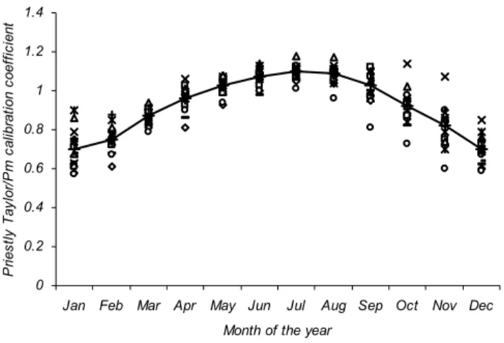
Van Kraalingen and Stol (1997) found that application of the Priestly-Taylor equation during the Dutch winter months was not possible because it is based on net radiation. Since net radiation is often negative in the winter, it predicts dew formation, whereas the actual ET is positive. The situation would be different for a humid climate such as the Philippines, or in a semi-arid climate such as Israel, where the equation should compare well with PM. Irmak et al. (2003) calibrated the Priestly-Taylor method against the FAO PM method using 15 years of climate data (1980–1994) in humid Florida, United States. The monthly values of the calibration coefficient (Fig. 5) show a considerable seasonal variation, aside from the natural difference in annual values. In general, the calibration coefficients are lower in winter months indicating that the Priestley and Taylor method underestimates ETo, and they are higher than 1.0 during the summer months, indicating that the method overestimates during the summer months. The long-term average lowest calibration values were obtained in January and December (0.70) and the highest values in July (1.10). These results indicate the importance of developing monthly calibration coefficients for regional use based on historic records. For the semi-arid conditions of southern Portugal, the authors also observed that the Priestley-Taylor method over-estimates daily ETo during the summer months (Shahidian et al., 2007).

Shuttleworth and Calder (1979) showed that Priestley-Taylor significantly underestimates wet forest evaporation, but also overestimates dry forest transpiration by as much as 20%. Berengena and Gavilán (2005) found that the Priestley–Taylor equation shows a considerable tendency to underestimate ETo, on average 23%, under convective conditions.

They concluded that the Priestly-Taylor equation is very sensitive to advection, and local calibration does not ensure an acceptable level of accuracy.

0 0.2 0.4 0.6 0.8 1 1.2 1.4

Jan Feb Mar Apr May Jun Jul Aug Sep Oct Nov Dec

Month of the year

P rie st ly T ayl or /P m ca lib ra tio n co ef fic ie nt

Fig. 5. Average monthly calibration coefficient for the Priestly-Taylor equation against PM for humid southern United States (based on data from Irmak et al. 2003).

3.2 The Makkink method

The Makkink method can be seen as a simplified form of the Priestley-Taylor method and was developed for grass lands in Holland. The difference is that the Makkink method uses incoming short-wave radiation Rs and temperature, instead of using net radiation, Rn, and temperature. This is possible, because on average, there is a constant ratio of 50% between net radiation and short wave radiation. The equation can be expressed as:

2,45 s o R Et         (18)

where  is usually 0.61, and  is -0.012. Doorenbos and Pruitt (1975) proposed the FAO Radiation method based on the Makkink equation (1957), introducing a correction factor based on estimates for wind and humidity conditions to compensate for advective conditions. This radiation method has been proven valid, in particular under humid conditions, but can differ systematically from the PM reference method under special conditions, such as during dry months (Bruin and Lablands, 1998).

It has also been observed that it is difficult to use this radiation based method during winter months: Van Kraalingen and Stol (1997) found that application of the Makkink equation in Dutch winter months was not possible, though the Makkink equation did not produce negative values for ET, as was the case with the Priestley-Taylor method. Bruin and Lablans (1998) also concluded that there is no relationship between Makkink and PM in the winter months, December and January, since Makkink's method has no physical meaning, in this period.

It is reasonable to expect the Makkink and the Priestley-Taylor equations to compare well with the Penman's method, since in all these approaches the radiation terms are dominant and radiation is the main driving force for evaporation in short vegetation.

ET models tend to perform best in climates in which they were designed. A study by Amayta et al. (1995) showed that while the Makkink model generally performed well in North Carolina, the model underestimated ETo in the peak months of summer. Yet, the Makkink model shows excellent results in Western Europe where it was designed, both in comparison to PM as well as to the measured ETo data (Bruin and Lablans 1998, Xu and Singh 2000, Bruin and Stricker 2000, Barnett et al., 1998).

3.3 The Turc method

Also known as the Turc-Radiation equation, this method was presented by Turc in 1961, using data from the humid climate of Western Europe (France). This method only uses two parameters, average daily radiation and temperature and for RH>50% can be expressed as:









And for RH < 50% as:









Where  is 0.01333 and Rs is expressed in MJ m-2 _day-1_.

Yoder et al. (2005) compared six different ET equations in humid southeast United States, and found the Turc equation to be second best only to the full PM. Jensen et al. (1990) analyzed the properties of twenty different methods against carefully selected lysimeter data from eleven stations, located worldwide in different climates. They observed that the Turc method compared very favorably with combination methods at the humid lysimeter locations. The Turc method was ranked second when only humid locations were considered, with only the Penman-Monteith method performing better. Trajkovic and Stojnic (2007) compared the Turc method with full PM in 52 European sites and found a SEE (Standard Error of Estimate) of between 0.10 and 0.37 mm d-1_{. They also found that the}

reliability of the Turc method depends on the wind speed (Fig. 6). The Turc method overestimated PM ETo in windless locations and generally underestimated ETo in windy locations.

Amatya et al. (1995) compared 5 different ETo methodologies in North Carolina and concluded that the Turc and the Priestley-Taylor methods were generally the best in estimating ETo. They observed that all other radiation methods and the temperature based Thorntwaite method underestimated the annual ET by as much as 16%.

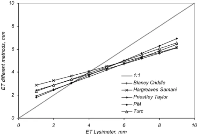
Kashyap and Panda (2001) compared 10 different methods with lysimeter data in the sub humid Kharagupur region of India and observed that the Turc method had a deviation of only 2.72% from lysimeter values, followed by Blaney-Criddle with a 3.16% and Priestly Taylor with a 6.28% deviation (Fig. 7). The Kashyap and Panda data are also important because they show that under sub humid conditions, most of the equations, including the PM, tend to overestimate when evapotranspiration is low, and underestimate when it is high.

y = 0.9838x0.0935 R2 _{= 0.6747} 0.6 0.7 0.8 0.9 1 1.1 1.2 1.3 1.4 0 0.5 1 1.5 2 2.5 3 3.5 Wind speed, m s-1 R at io of F A O -P M / T ur c

Fig. 6. Effect of wind on the ratio of evapotranspiration calculated with the FAO PM and the Turc methods (based on data from Trajkovic and Stojnic (2007), using average annual values). 0 2 4 6 8 10 0 2 4 6 8 10 ET Lysimeter, mm E T di ff er ent m et hods , m m 1:1 Blaney Criddle Hargreaves Samani Priestley Taylor PM Turc

Fig. 7. Comparison of various ETo methods with Lysimeter readings in the sub-humid region of Kharagpur, India (adapted from Kashyap and Panda, 2001).

For Florida, Martinez and Thepadia (2010) compared the reduced-set PM equation with various temperature and radiation based equations and concluded that in the absence of regionally calibrated methods, the Turc equation has the least error and bias when using measured maximum and minimum temperatures. They also observed that the reduced-set PM and Hargreaves equations overestimate ET.

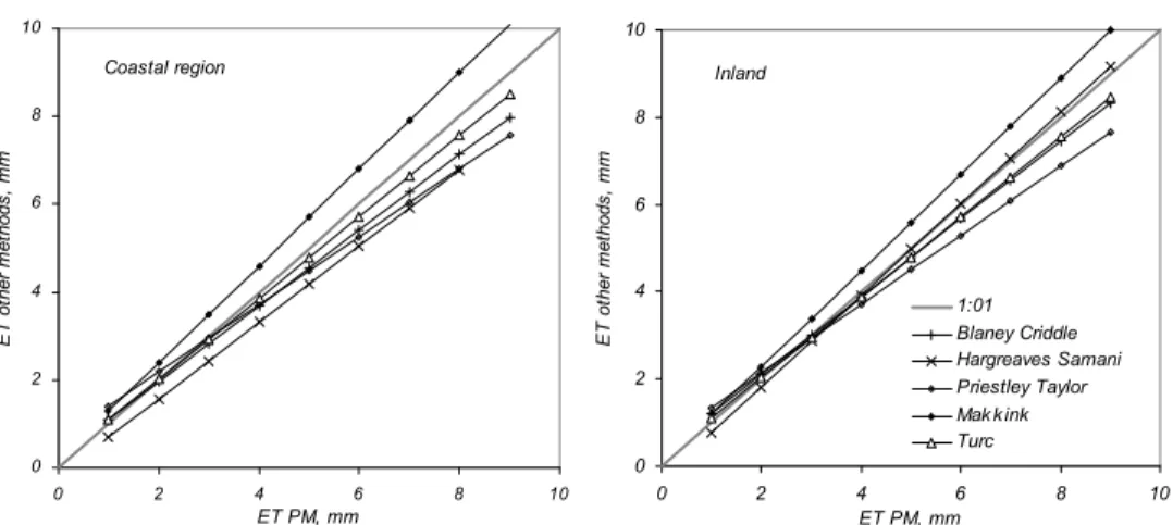
Fontenote (2004) studied the accuracy of seven evapotranspiraiton models for estimating grass reference ET in Louisiana. He observed that, statewide and in the coastal region, the Turc model was the most accurate daily model with a MAE of 0.26mm day-1_{. Inland, the}

Blaney-Criddle performed best with a MAE of 0.31mm day-1 _{(Fig. 8).}

Hence, it can be safely concluded that the Turc model can be expected to perform well in warm, humid climates such as those found in North Carolina (Amatya et al., 1995), India (George et al., 2002), and Florida (Irmak et al., 2003; Martinez and Thepadia, 2010).

0 2 4 6 8 10 0 2 4 6 8 10 ET PM, mm E T ot her m et hods , m m 1:01 Blaney Criddle Hargreaves Samani Priestley Taylor Mak kink Turc Inland 0 2 4 6 8 10 0 2 4 6 8 10 ET PM, mm E T ot her m et hods , m m Coastal region

Fig. 8. Comparison of five ET methods with PM in two different regions of Louisiana (Adapted from Fontenote, 1999).

3.4 The Jensen and Haise method

This method was derived for the drier parts of the United States and is based on 3,000 observations of ET. Jensen and Haise used 35 years of measured evapotranspiration and solar radiation to derive the equation, based on the assumption that net radiation is more closely related to ET than other variables such as air temperature and humidity (Jensen and Haise, 1965). The equation can be expressed as:





t x s

ET C T T R  (21)

The original study of Jensen and Haise provides a calculation procedure to obtain Rs from the cloudiness, Cl, and the solar and sky radiation flux on cloudless days. The temperature Constant, Ct, and the intercept of the temperature exis, Tx, can be calculated as follows:





















where h is the altitude of the location in m, Rs is solar radiation (MJ m-2 _d-1_{); e}o_{Tmax and e}o_Tmin

are vapour pressures of the month with the mean maximum temperature and the month with the mean minimum temperature, respectively, expressed in mbar.

For the humid and rainy Rio Grande watershed in Brazil, Pereira et al. (2009) compared 10 different equations and concluded that the methods based on solar radiation are more accurate than those based only on air temperature, with the Jensen and Haise method presenting the smallest MBE, and thus being the method most recommended for this region.

4. Conclusions

Both temperature and radiation can be used successfully to calculate daily ETo values with relative accuracy. All the equations can be used for areas that have a climate that is similar to the one for which the equations were originally developed; while most of the equations can be used with some confidence for areas with moderate conditions of humidity and wind speed.

Regional calibration, especially if including monthly calibration coefficients, is important in decreasing the bias of the ETo estimates. Wind speed can greatly influence the results obtained with reduced-set equations, since wind removes the boundary layer from the leaf surface and can significantly increase evapotranspiration. Relative Humidity is another important factor that can affect the results.

Globally, it is observed that the Turc equation is highly recommended for humid or semi-humid areas, where it can produce very good results even without calibration, while the Thornthwaite equation tends to underestimate ETo.

The Priestley-Taylor and the Makkinik equations should not be used in the winter months in locations with high latitude, such as northern Europe.

Both the Hargreaves and the reduced-set Panman-Monteith can be effectively used with only temperature measurements, although the results can be improved if wind speed is taken into consideration.

The use of the reduced-set equations can be very important in actual irrigation management, since the error involved in using these equations can be much smaller than that resulting from using data from a weather station located many miles away.

5. References

Allen RG (1993) Evaluation of a temperature difference method for computing grass reference evapotranspiration. Report submitted to the Water Resources Develop. and Man. Serv., Land and Water Develop. Div., FAO, Rome. 49 p.

Allen RG, Pereira LS, Raes D, Smith M (1998) Crop evapotranspiration: Guidelines for computing crop requirements. Irrigation and Drainage Paper No. 56, FAO, Rome, Italy.

Amatya DM, Skaggs RW, Gregory JD(1995) Comparison of Methods for Estimating REF-ET. Journal of Irrigation and Drainage Engineering 121:427-435.

Bautista F, Bautista D, Delgado-Carranza (2009) Calibration of the equations of Hargreaves and Thornthwaite to estimate the potential evapotranspiration in semi-arid and sub-humid tropical climates for regional applications. Atmósfera 22(4): 331-348 Berengena J, Gavilán P (2005) Reference evapotranspiration estimation in a highly advective

semiarid environment. J. Irrig. Drain. Eng. ASCE 131 (2):147–163.

Borges AC, Mendiondo EM (2007) Comparação entre equações empíricas para estimativa da evapotranspiração de referência na Bacia do Rio Jacupiranga. Revista Brasileira de Engenharia Agrícola e Ambiental 11(3): 293–300.

Blaney, HF, Criddle, WD (1950). Determining water requirements in irrigated áreas from climatological and irrigation data. In ISDA Soil Conserv. Serv., SCS-TP-96,

Blaney HF, Criddle WD. (1962). Determining Consumptive Use and Irrigation Water Requirements. USDA Technical Bulletin 1275, US Department of Agriculture, Beltsvill

Bruin, HAR Lablans, WN, (1998) Reference crop evapotranspiration determined with a modified Makkink equation. Hydrological Processes

Brutsaert, W (1991) Evapotration into the atmosphere. D. Reidel Publishing Company. DehghaniSanij H, Yamamoto T, Rasiah V (2004) Assessment of evapotranspiration

estimation models for use in semi-arid environments. Agricultural Water Management 64: 91–106

Hargreaves, G.H. (1994). Simplified coefficients for estimating monthly solar radiation in North America and Europe. Departmental Paper, Dept. of Biol. And Irrig. Engrg., Utah State University, Logan, Utah

Doorenbos J., Pruit WO. (1977) Guidelines for predicting crop water requirements. FAO irrigation and drainagem paper, 24

Droogers P, Allen, RG (2002) Estimating reference evapotranspiration under inaccurate data conditions. Irrig. Drain. Syst. 16(1): 33-45.

Fontenot Rl (2004) An evaluation of reference evapotranspiration models in Louisiana, MSc thesis, Louisiana State University, August.

Garcia M, Raes D, Allen R, Herbas C, (2004) Dynamics of reference evapotranspiration in the Bolivian highlands (Altiplano). Agric. Forest Meteorol. 125: 67–82.

George BA, Reddy BRS, Raghuvanshi NS, Wallender WW (2002) Decision support system for estimating reference evapotranspiration. J. Irrig. Drain. Eng. 128(1): 1–10. Hargreaves GH, Samni ZA. (1982) Estimation of potential evapotranspiration. Journal of

Irrigation and Drainage Division, Proceedings of the American Society of Civil Engineers 108: 223-230

Hargreaves GH, Samani ZA. (1985) Reference crop evapotranspiration from temperature. Appl Engine Agric. 1(2):96–99.

Hargreaves GH, Allen RG (2003) History and Evaluation of Hargreaves Evapotranspiration Equation. Journal of Irrigation and Drainage Engineering129(1): 53-63.

Henggeler J.C., Z. Samani, M.S. Flynn, J.W. Zeitler (1996) Evaluation of various evapotranspiration equations for Texas and New Mexico. Proceeding of Irrigation Association International Conference, San Antonio, Texas

Igbadun H, Mahoo H, Tarimo A, Salim B (2006) Performance of Two Temperature-Based Reference Evapotranspiration Models in the Mkoji Sub-Catchment in Tanzania. Agricultural Engineering International: the CIGR Ejournal. Manuscript LW 05 008. Vol. VIII. March,

Irmak S, Irmak A, Allen RG, Jones JW (2003) Solar and Net Radiation-Based Equations to Estimate Reference Evapotranspiration in Humid Climates. Journal of irrigation and drainage engineering. September/October

Irmak S, Istanbulluoglu, E, Irmak A. (2008) An Evaluation of Evapotranspiration model complexity against performance in comparison with Bowen Ration Energy Balance measurements. Transactions of the ASABE 51(4):1295-1310

Jabloun M, Sahli A (2007) Ajustement de l’e´quation de Hargreaves-Samani aux conditions climatiques de 23 stations climatologiques Tunisiennes. Bulletin Technique no. 2. Laboratoire de Bioclimatologie, Institut National Agronomique de Tunisie, 21 p. Jabloun M, Sahli A (2008) Evaluation of FAO-56 methodology for estimating reference

evapotranspiration using limited climatic data. Application to Tunisia. Agricultural Water Management 95: 707-715.

Jensen ME, Haise HR (1963) Estimating evapotranspiration from solar radiation. Journal of Irrigation and Drainage Division, Proc. Amer. Soc. Civil Eng. 89:15–41.

Jensen DT, Hargreaves GH, Temesgen B, Allen RG (1997) Computation of ETo under non ideal conditions. J. Irrig. Drain. Eng. ASCE 123 (5): 394–400.

Kashyap PS, Panda RK (2001) Evaluation of evapotranspiration estimation methods and development of crop-coefficients for potato crop in a sub-humid region. Agricultural Water Management 50: 9-25

López-Urrea R, Martín de Santa Olalla F, Fabeiro C, Moratalla A (2006) Testing evapotranspiration equations using lysimeter observations in a semiarid climate. Agricultural Water Management 85: 15–26.

Lu, J, Sun G, McNulty S, Amatya DM (2005) A Comparison of Six Potential Evapotranspiration Methods for Regional Use in the Southeastern United States. Journal of the American Water Resources Association (JAWRA) 41(3):621-633. Makkink GF. (1957) Testing the Penman formula by means of lysimeters. Journal of the

Institution of Water Engineers 11: 277-28

Martinez, A.M., Thepadia, M. (2010) Estimating Reference Evapotranspiration with Minimum Data in Florida. J. Irrig. Drain. Eng. 136(7): 494-501

McKenney, M. S. and N. J. Rosenberg, (1993) Sensitivity of some potential evapotranspiration estimation methods to climate change. - Agricultural and Forest Meteorology 64, 81-110.

Mohan S, Arumugam N (1996) Relative importance of meteorological variables in evapotranspiration: Factor analysis approach. Water Resour. Manage. 10, 1–20. Nandagiri L, Kovoor GM (2006) Performance Evaluation of Reference Evapotranspiration

Equations across a Range of Indian Climates. Journal of Irrigation and Drainage Engineering 132(3) . DOI: 10.1061/(ASCE)0733-9437(2006)132:3(238)

Oliveira RZ, Oliveira LFC, Wehr TR, Borges LB, Bonomo R (2005) Comparative study of estimative models for reference evapotranspiration for the region of Goiânia, Go. Biosci. J. Uberlândia, 21(3):19-27.

Paes de Camargo, A. and Paes de Camargo, M.(2000) Numa revisão analítica da evapotranspiração potencial Bragantia. Campinas 59 2, pp. 125–137.

Penman, H.L. (1948) Natural evaporation from open water, bare soil, and grass. Proc. Roy. Soc. London A193:120-146.

Pereira DR, Yanagi SNM, Mello CR, Silva AM, Silva LA (2009) Performance of the reference evapotranspiration estimating methods for the Mantiqueira range region, MG, Brazil. Ciência Rural, Santa Maria 39(9):2488-2493.

Priestley CHB, Taylor RJ (1972) On the assessment of the surface heat flux and evaporation using large-scale parameters. Monthly Weather Review 100: 81–92

Popova Z, Kercheva M, Pereira LS (2006) Validation of the FAO methodology for computing ETo with limited data. Application to south Bulgaria. Irrig Drain. 55:201–215. Rahimikhoob AR (2008) Comparative study of Hargreaves’s and artificial neural network’s

methodologies in estimating reference evapotranspiration in a semiarid environment. Irrig Sci 26:253–259.

Reis EF, Bragança R, Garcia GO, Pezzopane JEM, Tagliaferre C (2007) Comparative study of the estimate of evaporate transpiration regarding the three locality state of Espirito Santo during the dry period. IDESIA (Chile) 25(3) 75-84

Samani Z (2000) Estimating solar radiation and evapotranspiration using minimum climatological data. J Irrig Drain Engin. 126(4):265–267.

Samani ZA, Pessarakli M (1986) Estimating potential crop evapotranspiration with minimum data in Arizona. Trans. ASAE (29): 522–524.

Sepaskhah, AR, Razzaghi, FH (2009) Evaluation of the adjusted Thornthwaite and Hargreaves-Samani methods for estimation of daily evapotranspiration in a semi-arid region of Iran. Archives of Agronomy and Soil Science, 55: 1, 51- 6

Sentelhas C, Gillespie TJ, Santos EA (2010) Evaluation of FAO Penman–Monteith and alternative methods for estimating reference evapotranspiration with missing data in Southern Ontario, Canada. Agricultural Water Management 97: 635–644.

Shahidian, S., Serralheiro, R.P., Teixeira, J.L., Santos, F.L., Oliveira, M.R.G., Costa, J.L., Toureiro, C.. Haie, N. (2007) Desenvolvimento dum sistema de rega automático, autónomo e adaptativo. I Congreso Ibérico de Agroingeneria.

Shahidian S. , Serralheiro R. , Teixeira J.L., Santos F.L., Oliveira M.R., Costa J., Toureiro C., Haie N., Machado R. (2009) Drip Irrigation using a PLC based Adaptive Irrigation System WSEAS Transactions on Environment and Development, Vol 2- Feb. Shuttleworth, W.J., and I.R. Calder. (1979) Has the Priestley-Taylor equation any relevance

to the forest evaporation? Journal of Applied Meteorology, 18: 639-646.

Smith, M, R.G. Allen, J.L. Monteith, L.S. Pereira, A. Perrier, and W.O. Pruitt. (1992) Report on the expert consultation on procedures for revision of FAO guidelines for prediction of crop water requirements. Land and Water Development Division, United Nations Food and Agriculture Service, Rome, Italy

Stanhill, G., 1961. A comparison of methods of calculating potential evapotranspiration from climatic data. Isr. J. Agric. Res.: Bet-Dagan (11), 159–171.

Teixeira JL, Shahidian S, Rolim J (2008) Regional analysis and calibration for the South of Portugal of a simple evapotranspiration model for use in an autonomous landscape irrigation controller.

Thornthwaite CW (1948) An approach toward a rational classification of climate. Geograph Rev.38:55–94.

Trajkovic S. (2005) Temperature-based approaches for estimating reference evapotranspiration. J Irrig Drain Engineer. 131(4):316–323

Trajkovic S (2007) Hargreaves versus Penman-Monteith under Humid Conditions Journal of Irrigation and Drainage Engineering, Vol. 133, No. 1, February 1.

Trajkovic, S, Stojnic, V. (2007) Effect of wind speed on accuracy of Turc Method in a humid climate. Facta Universitatis. 5(2):107-113

Xu, CY, Singh, VP (2000) Evaluation and Generalization of Radiation-based Methods for Calculating Evaporation, Hydrolog. Processes 14: 339–349.

Xu CY, Singh VP (2002) Cross Comparison of Empirical Equations for Calculating Potential evapotranspiration with data from Switzerland. Water Resources Management 16: 197-219.