Classification of three-dimensional ocean features using three-dimensional empirical orthogonal functions

N´elson Martins

, Leandro Calado

, Ana C. de Paula

, S´ergio M. Jesus

1_{Institute for Systems and Robotics, University of Algarve, Campus de Gambelas, PT-8005-139 Faro, Portugal, {nmartins, sjesus}@ualg.pt} 2_{Institute of Marine Studies Admiral Paulo Moreira, Rua Kioto, 253, Praia dos Anjos, 28930-000 Arraial do Cabo, RJ, Brazil, {lcalado,}

ana.claudia}@ieapm.mar.mil.br

Acoustic tomography is now a well known method for remote estimation of water column properties. The problem is ill-conditioned and computationally intensive, if each spatial point varies freely in the inversion. Empirical orhogonal functions (EOFs) efficiently regularize the inversion, leading to a few (2, 3) coefficients to be estimated, giving a coherent estimate of the field. At small scales, EOFs are typically depth-dependent basis functions. The extension of the concept to larger-scale anisotropic fields requires horizontal discretization into cells, with corresponding coefficients. This becomes unstable and computationally intensive, having been overcome by two-dimensional depth-range EOFs, in the past. The present work extends the empirical orthogo-nal function concept to three dimensions, assessing the performance of the inversion for an instantaneous sound speed field constructed from dynamical predictions for Cabo Frio, Brazil. The results show that the large-scale features of the field are correctly estimated, though with strong ambiguity, using an acoustic source tens of km from an acoustic hydrophone array. Work is under progress, to remove the ambiguity and estimate finer details of the three-dimensional field, via the addition of multiple acoustic arrays.

1

Introduction

Acoustical oceanography has since the 70’s played an im-portant role in ocean exploration. Taking advantage of the ocean transparency to sound, the latter is used to study ocean physics and biology. Essentially, sound propagation carries information about the phenomenon to study, to an acous-tic system available to the researcher. Acousacous-tical oceanog-raphy has been successful in studying global warming, the sea bottom, suspendend sediments, bubble clouds, plumes, rainfall, sea surface roughness, gas interchange in breaking waves, and tracking whales, remotely measuring the shape and strength of internal waves, ocean eddies and other fea-tures[1]. Special interest has been given to the water co-lumn, from intermediate (tens of m–10 km) to large (>100 km) scales, through ocean acoustic tomography. Tomogra-phy (slice writing) is an imaging technique which inverts propagation measurements (differences in speed, attenua-tion, etc.) through many sections of a volume to determine its characteristics. Its earliest application was three-dimen-sional studies of human tissue density variation by the dif-ferential attenuation of X-rays. In 1979, Munk and Wun-sch suggested to apply this concept to obtain sound speed and infer temperatures in an ocean volume[2]. It appeared as an advantageous complementary means of ocean estima-tion, producing results in minutes–hours (a CTD survey can last 2 weeks), in a continuous manner. Tomography intrin-sically performs a low-pass filtering of the properties to ob-serve (giving integral measures), since it deals with the end points of propagation paths, and is sensitive to the accumu-lated acoustic impact of local properties. This characteristic is even exclusive from this remote sensing method, useful for climate studies, when applied to basin-scales, to mea-sure the variability of temperature and heat content in ocean

basins. The tomographic measurements often work as in-tegral constraints on general circulation models. By other words, tomography measurements are robust Eulerian mea-surements of the water column variability, with no calibra-tion drift. Acoustic tomography is sensitive to variability in ocean depths close to the ocean bottom, attaining depths below those reachable by XBT and floats.

Usually, in 3D (three-dimensional in space) tomography, the problem is divided into vertical-slice problems (borrowing concepts from medical scans), in which many slice-structures are estimated, to compose the final 3D estimate. Each verti-cal slice is designed at a strategic horizontal angle, requiring the deployment of more than one acoustic source or receiver array, to form a sufficiently large number of source-receiver paths, to define an unambiguous estimate. One advantage of tomography over non-acoustic approaches is that the num-ber of data points grows geometrically with the product no. of sources × no. of receivers, as opposed to their sum. A problem regarding the estimation of 3D fields is the large amount of physical parameters to be estimated (leading to underdetermination, if there are no sufficient independent measurements, and to a slow computation). Inverse theory can be used to constrain the solution to the smoothest field, or the unique solution consistent with a priori knowledge of the field covariance. An alternative approach is to reg-ularize the estimation problem, by expanding the field to be estimated into meaningful basis functions. When there are no ocean circulation models, one has to do optimal in-terpolation of sparse measures, with subjective parametriza-tions. Then, the problem consists of estimating the expan-sion coefficients. Typical basis functions are uniform, li-near and cubic splines, wavelets, vertical hydrodynamical modes, Fourier basis and principal components. The latter are called empirical orthogonal functions (EOFs), in the

me-tereology and underwater acoustics literature. EOFs are the most efficient representations, and their application is con-ditioned to statistical stationary fields. EOFs allow to filter out unwanted scales of variability, and to compress ocean-ographic data into a minimum number of patterns. Very of-ten, EOFs are computed to represent the depth-variability of ocean properties like temperature or sound speed.As a con-sequence, the ocean is divided into horizontally-invariant parallelepipeds, and a set of EOF coefficients for each par-allelepiped is estimated. EOFs can be computed from his-torical hydrographies, or, in their absence, from physical oceanography.

The very first 3D tomography experiment (Ocean Tomo-graphy Experiment) had as central goal the production of three-dimensional time-evolving maps of the ocean, using 4 sources and 5 receivers[3]. The ability to produce a 3D map (300 × 300 km) using acoustics alone was demonstra-ted.These ideas have been implemented in a number of suc-cessive tomography experiments, from which we can men-tion: Greenland Sea, in 1988–1989 (using 6 acoustic trans-ceivers in an array approximately 210 km in diameter); AMODE, in 1991 (using 6 acoustic-transceiver moorings within a cir-cle with a radius of 350 km); Heard Island Feasibility Test, in 1991, (a very-long-range transmission test to investigate the heating of the world’s oceans); THETIS I, in 1991, (us-ing 6 transceiver moor(us-ings separated by 100–200 km); Acous-tic Thermometry of Ocean Climate, in 1995 (for basin scale studies); Shelf Break Primer Experiment, in 1996 (using 4 depth-dependent EOFs). In [4], 2D (2-dimensional of depth and range) EOFs were used to study the large-scale varia-bility in the California Current System, employing a sound source ≈ 624 km from the receiver (a number of other ar-rays was also used).In [5], the upper ocean (a 10 by 10 km (in the horizontal) by 20 m (in depth) block) was expanded into distinct basis vectors for the along-shore, seaward and depth dimensions, with independent statistics between them. The upper layer could be represented accurately with only 2 nonzero EOF coefficients, to less than 0.01 m/s maximum error at any point. An (inexpensive) single source-receiver pair was used successfully to estimate the 3D upper layer structure, in simulations, using a 500 Hz source 10 km apart from the receiver.

The work at hand presents a single-acoustic slice tomographic approach for the 3D ocean, in which the EOFs are defined for the 3D space, assuming dependent statistics in all 3 di-mensions, and covering an area of ≈ 40 by 80 km (in the horizontal) by 171 m (in depth). The next section formu-lates the problem, and is followed by the results with simu-lated acoustic data, and the conclusions.

2

Problem statement and background

The present work concerns the estimation of the three-di-mensional spatial (at longitude x, latitude y and depth z) sound speed field (c) evolution with time (t), at M locations of an oceanic volume of interest, by means of acoustic in-version. The field is approximated by an empirical orthog-onal function decomposition, whose time-dependent

coef-ficients —grouped into the vector θT(t)— are to be

esti-mated. The underlying technique assumes that the volume is probed with broadband acoustic signals (at L frequencies), propagating from a source to a set of vertical hydrophone arrays, and then being inverted for the required coefficients. The following sections review the concept of empirical or-thogonal function, and the acoustic inversion technique used in deriving the results.

2.1

Empirical orthogonal functions

Many analyses of climate data sets suffer from high dimen-sions of the variables representing the state of the underlying system at any given time, demanding for a split of the full phase space into two subspaces.

The “signal subspace” is supposed to represent the dynamics of the process, while the “noise subspace” contains all pro-cesses which are supposedly irrelevant in their details for the “signal subspace” (including uncertainties introduced by the measurement or objective analyses). The signal subspace is spanned by few characteristic patterns, and has longer scales in time and space, and fewer degrees of freedom, than the noise subspace.

Let us assume that we have at hand observations of the M -point field evolution, whose representation in terms of “sig-nal” (spanned by sk) and “noise (spanned by n(t)) subspaces”

may be written as x(t) = K X k=1 αk(t) sk+ n(t), (1) with K ≤ M .

It is assumed that any time-dependent vector x(t) is a real-ization of a common zero-mean random variable X, with

co-variance matrix Σ and co-variance var(X) =P

mE[X 2

m], m =

1, . . . , M , i.e., the observations represent field anomalies. Empirical orthogonal functions (EOFs, termed in [6], or prin-cipal vectorsor loadings) are defined as that set of K

ortho-normal vectors which span the same space as sk, and

mini-mize the variance of the residual n(t) in Eq. (1) (thus acting as a ‘misfit’ minimization).

The EOFs are the eigenvectors of Σ associated with the largest

eigenvalues λk. The expansion coefficients αk = xTvk

(sometimes labelled principal components or scores) are uni-variate random variables.

They are uncorrelated:

E[αkαl] = λkδkl, (2)

with δkl the Kronecker delta. We could say that the EOFs

statistically synthesize the joint time variability of physical quantities (some approaches work in the frequency domain instead).

The variance of n(t) can be defined as a dot product in one of different metrics, rendering the definition of EOF metric-dependent.

Regarding the choice of K, for which, a good answer is case-dependent, one usually defines a criterion built on the proportion of X-variance accounted for by the EOFs. This measure can be calculated for individual EOFs, or sets of EOFs, ηk= λk PM m=1λm , or η1,2,...,K= PK k=1λk PM m=1λm , (3)

and is formally similar to the Brier-based score[7]. K is of-ten selected according to one of two criteria: either the per-centage of X-variance explained by the first K EOFs passes a certain threshold, or the last kept EOF accounts for a cer-tain minimum variance:

η1,...,K≤ κ1< η1,...,K+1, or ηK > κ2> ηK+1. (4)

Typical values for κ1 are 80% or 90%, and for κ2, 5% or

1%.

In practical situations, the covariance matrix Σ is unknown, and typically, the EOFs are estimated from a finite sample {x(1), . . . , x(N )}, as the eigenvectors of the data covariance matrix. This is why EOFs are called “empirical” (reflecting the fact that they are estimated from the specific data set being analyzed, whose dynamics is sometimes unknown). The first EOF or few EOFs may represent a meaningful physical summary of relevant processes, the same holding for the remaining EOFs only under very special circum-stances —in most real-world cases, processes are not uncor-related, and may be described by meaningful non-orthogonal patterns.

2.2

Acoustic inversion

Consider the complex acoustic pressures from measures by all the hydrophones of the H-hydrophone A vertical arrays,

grouped into the vector p(f, θT), function of frequency f

and the (true) vector of EOF coefficients θT(t) (t dropped).

Acoustic inversion, in the present work, consists of find-ing the EOF coefficients in θ that maximize the ‘acous-tic correlation function’ given by the broadband frequency-incoherent Bartlett power (a generalization of the plane-wave beamformer) BBart(θ) = 1 K K X k=1 wH(f, θ) ˆK(f, θT) w(f, θ), (5)

whereHis the Hermitian operator, and ˆK(f, θT) is an

esti-mate of the correlation matrix of p(f, θT). For each

candi-date vector θ, the unit-norm vector w = [w1, w2, . . . , wHA]T

of calculated pressure on the A vertical arrays is computed. The search in θ is carried out exhaustively.

3

Results

The results consider the inversion for a synthetic time-evolv-ing three-dimensional sound speed field off Cabo Frio, Bra-zil. The oceanography of Brazil is essentially determined

by the Brazil Current (BC) system. In the 20–28◦S range,

the BC has been reported in the literature as a weak shallow, warm and salty southward flowing western boundary cur-rent, which develops intense mesoscale activity. Evidence of large nearly standing frontal cyclonic meanders, north from Cabo Frio, can be given by satellite images, pointing Cabo de S˜ao Tom´e (22◦S) as a vortex activity birth point, attributed to the sharp change in the coastline[8]. Another feature of interest is the upwelling activity along the zonal coast south from Cabo Frio.

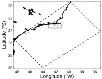
In the present work, an ocean dynamics simulation for the brazilian southeast coast was carried out using the Regional Ocean Modeling System (ROMS), from which the box with corners (23◦28.46’S, 42◦26.48’W) and (23◦07.16’S, 41◦39 .52’W) (an ≈ 55.6 × 204 km box) was selected for analysis

—see fig. 1. ROMS is a free-surface, terrain-following,

48 46 44 42 40 38 36 30 28 26 24 22 20

Longitude (

°

W)

Latitude (

°

S)

Figure 1: Boxes considered for the: Regional Ocean Model-ing System run (dashed line) and acoustic inversion exercise (continuous line), for the Cabo Frio (circle center) simula-tion.

primitive equations ocean circulation model widely used by the scientific community for a diverse range of applications [9]. ROMS includes several coupled models for biogeo-chemical, bio-optical, sediment and sea ice applications, and vertical mixing schemes, multiple levels of nesting and com-posed grids. Prior to tackling the problem at hand, the model was run to issue forecasts for the whole year of 2009, with one-day spaced results, using thermohaline climatologies and real daily winds. For analysis, only the period 1st

De-cember–31stDecember was considered. Noiseless acoustic

data at frequencies 500 and 1000 Hz was synthesized, us-ing the adiabatic approximation in a range-dependent im-plementation of the SNAP code[10]. Then, the matched-field processor in Eq. (5) was applied to the data, in order to recover the field evolution. The search for the physical parameters was carried out using a genetic algorithm.

3.1

Simulation setup

The volumetric empirical orthogonal functions EOFk(x, y,

z), k = 1, . . . , K were computed by the standard technique explained in sec. 2.1, using the daily field evolution derived by ROMS at M spatial locations inside the box in fig. 1, with a resolution of 0.786 km × 2.06 km × 1 m in latitude, longitude and depth, respectively, during the December pe-riod. In order to obtain a detailed representation of the sound speed field, 8 EOFs were used, corresponding to a value of κ1= 80% in the criteria in Eq. (4).

In order to assess the possibility of estimating 3D sound speed fields, using a single acoustic source and receiver, dif-ferent geometries for the acoustic system were tested, to

es-timate the oceanographic feature given for 31st _December.

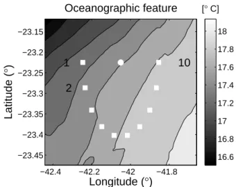
The source was positioned at 20-m depth, and the receiver consists of a 1–46 m depth 10-hydrophone array. The tested positions are shown in fig. 2, superposed to the 1-m depth representation of the feature to estimate, and refer to 1 sam-pled arc representing a source-receiver distance of 20 km, respectively.

Longitude (

°

)

Latitude (

°

)

Oceanographic feature

1

2

10

Figure 2: Horizontal section at 1-m depth of the 3D ocean-ographic feature to be estimated by acoustic inversion. The circle represents the acoustic source, and the squares, each of the tested receiver positions (numbered as suggested by the indicated ones).

In analyzing the acoustic inversion results, it is worth first to separate the possible estimation errors. Two main errors can be identified. The first is systematic and due to the EOF approximation (8 EOFs, as compared to N = 31 snapshots of the sound speed field), with the implicit error as in eq. 1, here associated to a 80% of ‘explained variance’. The second error is more subtle, and due to the random character of the search algorithm (genetic algorithm), which does not guarantee that the global maximum of function (5) will be ‘attained’ during the inversion.

In carrying out the acoustic inversion exercise, only the cor-responding vertical sections of the volumetric EOFs will act as basis functions to generate the sound speed field

sec-tion. This is because the acoustic propagation model as-sumes cylindrical geometry.

In fig. 3, the estimation results for the acoustic transects with indices 1, 3, 5, 7 and 9 (see fig. 2) are shown. We can

True Estimated Error

Transect 1 Depth [m] 0 50 100 150 10 12 14 16 10 12 14 16 0 5 10 15 −0.1 0 0.1 Transect 3 Depth [m] 0 50 100 150 10 12 14 16 10 12 14 16 0 5 10 15 −0.1 0 0.1 Transect 5 Depth [m] 0 50 100 150 10 12 14 16 10 12 14 16 0 5 10 15 −0.1 0 0.1 Transect 7 Depth [m] 0 50 100 150 10 12 14 16 10 12 14 16 0 5 10 15 −0.1 0 0.1 Transect 9 Range (km) Depth [m] 0 5 10 15 0 50 100 150 10 12 14 16 Range (km) 0 5 10 15 10 12 14 16 Range (km) 0 5 10 15 −0.1 0 0.1

Figure 3: True (left column), estimated (middle column) and estimate error (right column) in temperature (deduced from the sound speed estimate) along the transects 1, 3, 5, 7 and 9 (defined as in fig. 2). All temperatures are given in◦C.

see that the sound speed estimate corresponds to a

transect-temperature error always less than 0.2◦C. We can see that

the estimates agree well with the true feature characteristics, over depth. An histogram of the error amplitude at 171-m depth (not shown) was computed, showing a mode inferior to 0.03◦C.

4

Summary

The results show that the acoustic inversion for the three-di-mensional (3D) sound speed field is feasible with a moderate-to-reduced number of acoustic sensors, by expanding the field into 3D spatial empirical orthogonal functions (EOFs).

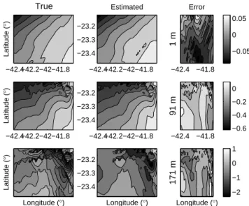
Latitude ( ° ) True −42.4−42.2−42−41.8 Estimated −42.4−42.2−42−41.8 −23.4 −23.3 −23.2 1 m Error −42.4 −41.8 −0.05 0 0.05 Latitude ( ° ) −42.4−42.2−42−41.8 −42.4−42.2−42−41.8 −23.4 −23.3 −23.2 91 m −42.4 −41.8 −0.6 −0.4 −0.2 0 Latitude ( ° ) Longitude (°) Longitude (°) −23.4 −23.3 −23.2 171 m Longitude (°) −2 −1 0 1

Figure 4: Temperature signatures: true (first column), esti-mated (second column) and estimate error (third column), at three depths: 1, 91 and 171 m (first, second and third lines, respectively), as a function of latitude and longitude. The estimates were obtained when the acoustic source and re-ceiver assumed the points of transect no. 3, in fig. 2. The color scales in the first two columns are coincident. At 1-m depth, the true signature is coincident with the one in fig. 2. All temperatures are expressed in◦C.

The definition of 3D EOFs, which synthesize the combined spatial variability of the field, allows for a single-slice alter-native to the traditional multi-slice tomography concept for oceanic volumes, with a relatively low computational cost. For the particular area of Cabo Frio, it was seen that, by using the frequencies 500 and 1000 Hz, propagated to a 10-hydrophone array 20 km away from the acoustic source, an oceanic volume of 40 × 80 km (horizontal dimensions) × 171 m (in depth) could be recovered for its sound speed field (and/or temperature), with a small error in temperature, es-sentially independent from the transect of the acoustic obser-vation. This was confirmed by looking at the results obtai-ned for the acoustic observation in the transect in which the sound speed is only mildly range-dependent, allowing to re-cover the full three-dimensional oceanographic fields, well away from the acoustic source/receiver. The main characte-ristics of the analyzed oceanographic feature were estimated with acceptable quality, with estimate errors very often less than 0.5◦C in temperature. The accuracy of the results can only be judged upon their application, and have to be ap-preciated according to either oceanographic (with varying scales of interest) or acoustic applications.

The present technique is highly dependent on the existence and performance of an ocean dynamical model, which al-lows to derive the cross-statistics of the spatial variability of the field to estimate, allowing for the definition of the 3D empirical orthogonal functions as bases with coefficients to estimate. A priori, the presented results can be improved, by using multi-slice acoustic configurations. These

configura-tions will be tested, and the acoustic signals received in the multiple hydrophone arrays will be processed coherently, in a single step, in order to reduce the estimation uncertainty. According to the presented results, it is expected that, if the EOF basis well represents the instantaneous field to esti-mate, the latter can be recovered with a minimal number of slices, with an increased accuracy with respect to the pre-sented single-slice case. Equivalently, it is expected that the same accuracy as in traditional volumetric tomographic ap-proaches can be attained with a smaller number of slices, compensated by the 3D coherence of 3D EOFs.

Acknowledgements

This work was partially supported by the project WEAM (PTDC/ENR/70452/2006) and the scholarship SFRH/BD/ 9032/2002, from FCT, Portugal, and the EU OAEx Marie Curie FP7 230855 Program.

References

[1] A. Kaneko, G. Yuan, N. Gohda, and I. Nakano.

Op-timum design of the ocean acoustic tomography sys-tem for the Sea of Japan. Journal of Oceanography, 50(3):281–293, May 1994.

[2] W.H. Munk and C. Wunsch. Ocean acoustic

tomogra-phy: a scheme for large scale monitoring. Deep-Sea Research, 26 A:123–161, 1979.

[3] Ocean Tomography Group. A demonstration of ocean

acoustic tomography. Nature, 299:121–125, 1982.

[4] S.-K. Han, C. Collins, C. Miller, C.-S. Chiu, and

P. Worcester. Mapping the regional variability of the California Current acoustically using a waveform in-version method. J. Acoust. Soc. Am., 107(5):2862– 2862, 2000.

[5] Nicholas C. Makris, John S. Perkins, Scott P. Heckel,

and Josko Catipovic. Optimizing environmental

parametrization and experimental design for shallow water sound speed inversion, volume 12 of Modern ap-proaches in geophysics, pages 115–120. Kluwer aca-demic pub., 1995.

[6] E. Lorenz. Empirical orthogonal functions and

statis-tical weather prediction. Scientific report 1, Air Force Cambridge Research Center, Air Research and Devel-opment Command, Cambridge Mass., 1956.

[7] Antonio Navarra Hans von Storch, editor. Analysis of

Climate Variability: Applications of Statistical Techni-ques: Proceedings of an Autumn School Organized by the Commission of the European Community on Elba from October 30 to November 6, 1993. Springer,, 2 edition, 1999.

[8] E.J.D. Campos, J.E. Gonc¸alves, and Y. Ikeda. Water mass characteristics and geostrophic circulation in the South Brazil Bight —summer of 1991. J. Geophys. Res., 100(9):18,537–18,550, 1995.

[9] J.L. Wilkin, H.G. Arango, D.B. Haidvogel, C.S.

Licht-enwalner, S.M. Durski, and K.S. Hedstrom. A regional ocean modeling system for the Long-term Ecosystem Observatory. J. Geophys. Res., 110(C06S91), 2005. [10] F.B. Jensen and M.C. Ferla. SNAP: The

SACLANT-CEN normal-mode acoustic propagation model. Tech-nical Report SM-121, SACLANT Undersea Research Centre, La Spezia, Italy, 1979.