A computationally efficient model for the Greenland ice sheet

(1)

TCD

6, 2751–2788, 2012

A computationally efficient model for the

Greenland ice sheet

J. Haqq-Misra et al.

Title Page

Abstract Introduction

Conclusions References

Tables Figures

◭ ◮

Back Close

Full Screen / Esc

Printer-friendly Version

Interactive Discussion

Discussion

P

a

per

|

Dis

cussion

P

a

per

|

Discussion

P

a

per

|

Discussio

n

P

a

per

|

The Cryosphere Discuss., 6, 2751–2788, 2012 www.the-cryosphere-discuss.net/6/2751/2012/ doi:10.5194/tcd-6-2751-2012

The Cryosphere Discussions

This discussion paper is/has been under review for the journal The Cryosphere (TC). Please refer to the corresponding final paper in TC if available.

A computationally e

_ffi

cient model for the

Greenland ice sheet

J. Haqq-Misra1,*, P. Applegate2,3, B. Tuttle4, R. Nicholas2, and K. Keller2

1

Rock Ethics Institute, Pennsylvania State University, University Park, PA, USA 2

Department of Geosciences, Pennsylvania State University, University Park, PA, USA 3

Department of Physical Geography and Quaternary Geology (INK), Stockholm University, Stockholm, Sweden

4

Graduate Program in Acoustics, Pennsylvania State University, University Park, PA, USA *

now at: Blue Marble Space Institute of Science, Seattle, WA, USA

Received: 8 June 2012 – Accepted: 22 June 2012 – Published: 23 July 2012 Correspondence to: J. Haqq-Misra (jacob@bmsis.org)

Published by Copernicus Publications on behalf of the European Geosciences Union.

(2)

TCD

6, 2751–2788, 2012

Title Page

Tables Figures

◭ ◮

Back Close

Full Screen / Esc

Discussion

P

a

per

|

Dis

cussion

P

a

per

|

Discussion

P

a

per

|

Discussio

n

P

a

per

|

Abstract

We present a one-dimensional model of the Greenland Ice Sheet (GIS) for use in analysis of future sea level rise. Simulations using complex three-dimensional models suggest that the GIS may respond in a nonlinear manner to anthropogenic climate forcing and cause potentially nontrivial sea level rise. These GIS projections are,

how-5

ever, deeply uncertain. Analyzing these uncertainties is complicated by the substantial computational demand of the current generation of complex three-dimensional GIS models. As a result, it is typically computationally infeasible to perform the large num-ber of model evaluations required to carefully explore a multi-dimensional parameter space, to fuse models with observational constraints, or to assess risk-management

10

strategies in Integrated Assessment Models (IAMs) of climate change.

Here we introduce GLISTEN (GreenLand Ice Sheet ENhanced), a computationally efficient, mechanistically based, one-dimensional flow-line model of GIS mass balance capable of reproducing key instrumental and paleo-observations as well as emulating more complex models. GLISTEN is based on a simple model developed by Pattyn

15

(2006). We have updated and extended this original model by improving its compu-tational functionality and representation of physical processes such as precipitation, ablation, and basal sliding. The computational efficiency of GLISTEN enables a sys-tematic and extensive analysis of the GIS behavior across a wide range of relevant pa-rameters and can be used to represent a potential GIS threshold response in IAMs. We

20

demonstrate the utility of GLISTEN by performing a pre-calibration and analysis. We find that the added representation of processes in GLISTEN, along with pre-calibration of the model, considerably improves the hindcast skill of paleo-observations.

1 Introduction

The Greenland Ice Sheet (GIS) is a major feature of the Arctic and exerts a

poten-25

tially important control on future sea level change. The ice sheet covers an area of

(3)

TCD

6, 2751–2788, 2012

Title Page

Tables Figures

◭ ◮

Back Close

Full Screen / Esc

Discussion

P

a

per

|

Dis

cussion

P

a

per

|

Discussion

P

a

per

|

Discussio

n

P

a

per

|

1.7_×106km2 (Bamber et al., 2001), and has a maximum elevation of_∼3.3 km above sea level (Ekholm, 1996). Its reflective surface and height exert an important control over middle to high northern latitude climates (Toniazzo et al., 2004; Lunt et al., 2004). If the GIS were to melt completely, global sea level would rise by an average of approxi-mately seven meters (Bamber et al., 2001). Although Antarctica holds more ice (_∼60 m

5

sea level equivalent; Lythe et al., 2001), Greenland is often considered a more immedi-ate concern because large parts of its surface are already melting (Mote et al., 2007). In contrast, surface melting in Antarctica is largely restricted to the Antarctic Peninsula (Torinesi et al., 2003). Satellite measurements suggest that the GIS mass balance is already negative, and this negative trend may be accelerating (Velicogna, 2009; Alley

10

et al., 2010, and references therein).

Ice sheet model development has been particularly intensive since the Intergovern-mental Panel on Climate Change’s Fourth Assessment (Meehl et al., 2007), and many modeling experiments have analyzed the past and possible future behavior of the ice sheet (e.g. Greve, 1997, 2000; Huybrechts and de Wolde, 1999; Tarasov and Peltier,

15

2003; Lhomme et al., 2005; Stone et al., 2010; Greve et al., 2011; Robinson et al., 2011). Many GIS models are “shallow ice” approximation models, with representations of processes that are considered most significant in the real ice sheet. These models neglect important stress components within the ice body (Kirchner et al., 2011). Devel-opment and testing of models that resolve these additional stress terms is an area of

20

active research (e.g. Larour et al., 2012).

Although much effort today is given to the development of complex models, simplified but mechanistically based models can play an important role. In particular, integrated assessment models (IAMs) that describe the coupling between climate and economic growth require fast modules for the different parts of the Earth system, which includes

25

the GIS (e.g. Hulme et al., 1995). A fast ice sheet model also would be useful for exploring the effects of uncertain model parameters on hindcasts and projections of the ice sheet’s behavior (Robinson et al., 2011; Applegate et al., 2012). Simplified models have proven their usefulness in modeling other aspects of the climate system,

(4)

TCD

6, 2751–2788, 2012

Title Page

Tables Figures

◭ ◮

Back Close

Full Screen / Esc

Discussion

P

a

per

|

Dis

cussion

P

a

per

|

Discussion

P

a

per

|

Discussio

n

P

a

per

|

notably the El Ni ˜no-Southern Oscillation (Cane and Zebiak, 1985) and the meridional overturning circulation (Stommel, 1961; Keller et al., 2007).

To help address these needs, we present the GLISTEN (GreenLand Ice SheeT EN-hanced) model. This model is based on GRANTISM, a one-dimensional ice sheet model model by Pattyn (2006). GLISTEN resolves many processes that are important

5

for the real ice sheet. We update the original GRANTISM model with improved treat-ments of surface ablation and basal temperatures, and we include a parameterization of the Zwally effect (Zwally et al., 2002; Parizek and Alley, 2004). These treatments are highly parameterized, which allows for very quick model evaluation.

In this paper, we first provide a brief overview of the processes that affect GIS

be-10

havior and then provide a complete description of the GLISTEN model. We indicate specifically where GLISTEN is simplified relative to more complex three-dimensional

ice sheet models and where GLISTEN differs from GRANTISM. We then show that

GLISTEN successfully imitates a three-dimensional, shallow-ice model (SICOPOLIS; http://sicopolis.greveweb.net; Greve, 1997; Greve et al., 2011) and can reproduce

15

paleo- and instrumental observations. Finally, we discuss how this model can be ex-tended and implemented in IAMs.

2 A brief overview of ice sheet models

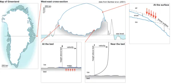
The GLISTEN model presented in this paper represents many processes considered important for the GIS. An illustration of some of these processes is shown in Fig. 1, with

20

glacier motion occuring as a result of internal deformation and basal sliding across the bedrock. Accumulation of ice and snow also primarily occurs at the center of the ice sheet, while ablation mainly occurs at the outer edges. This model is still consider-ably simplified, but it provides a rapid means of exploring GIS behavior that can be compared with more complex ice sheet models.

25

Perhaps the most complex components of an ice sheet model are the routines that calculate ice flow. The deformation of glacial ice is often assumed to follow a power-law

(5)

TCD

6, 2751–2788, 2012

Title Page

Tables Figures

◭ ◮

Back Close

Full Screen / Esc

Discussion

P

a

per

|

Dis

cussion

P

a

per

|

Discussion

P

a

per

|

Discussio

n

P

a

per

|

for fluid flow with an exponent of_∼3 (Glen, 1955; Nye, 1957; Cuffey and Kavanaugh, 2011, and references therein; cf. Goldsby and Kohlstedt, 2001); however, ice sheet ice is softer than the pure ice used in laboratory experiments, so a prefactor is used to match predictions from Glen’s flow law to observed behavior (e.g. Rutt et al., 2009). Many current ice sheet models solve the equations of ice flow using the shallow-ice

5

approximation (Hutter, 1983) and finite-difference solution methods over a grid that has a constant spacing in the horizontal plane but is scaled to ice thickness in the vertical direction. Examples of these shallow-ice models include SICOPOLIS (Greve, 1997; Greve et al., 2011) and Glimmer-CISM (Rutt et al., 2009). Both simpler and more complex solution methods exist. Velocities can be integrated vertically (e.g. Calov and

10

Marsiat, 1998), leading to a simpler problem. A few models use finite elements in-stead of finite differences, allowing refinement of the model mesh in crucial areas (e.g. Larour et al., 2012; Leng et al., 2012). Higher-order models resolve stress components that are neglected by the shallow-ice approximation (Kirchner et al., 2011), but usu-ally have significantly higher computing costs (e.g. Price et al., 2011; cf. Pollard and

15

DeConto, 2009). Examples of these higher-order models include ISSM (Larour et al., 2012), Elmer/Ice (Seddik et al., 2012), and some versions of Glimmer-CISM (Price et al., 2011). One promising approach involves applying full-Stokes solution methods only where they are necessary to maintain accuracy (Seroussi et al., 2010).

The dynamics of ice flow are fundamentally di_fferent in ice streams and ice shelves

20

than in places where the ice moves more slowly (MacAyeal et al., 1989; Kirchner et al., 2011). In slowly-moving grounded ice, deformation is controlled by vertical stresses; in ice streams and ice shelves, longitudinal stresses dominate. Ice margins in contact with water are highly vulnerable to mass loss from calving or basal melting. Removal of ice shelves also can cause tributary glaciers to speed up (e.g. Schmeltz et al., 2002;

25

Scambos et al., 2004; Dupont and Alley, 2005). Shallow-ice models simply neglect the problem of enhanced flow; others use the “shallow shelf approximation” in regions of fast flow (e.g. Bueler and Brown, 2009). Hybrid, higher-order, and full-Stokes models treat these features of the ice sheet “automatically,” rather than requiring a separate

(6)

TCD

6, 2751–2788, 2012

Title Page

Tables Figures

◭ ◮

Back Close

Full Screen / Esc

Discussion

P

a

per

|

Dis

cussion

P

a

per

|

Discussion

P

a

per

|

Discussio

n

P

a

per

|

module for fast-flow regions. Calving and ice shelf basal processes represent areas of active research (e.g. Alley et al., 2008; Walker et al., 2009).

Ice flow is sensitive to local temperature (Paterson and Budd, 1982; Greve and Blat-ter, 2009), and some thermal energy enters ice sheets from the bed (e.g. Dahl-Jensen and Gundestrup, 1987; Greve, 2005). Warmer ice deforms more readily than cold ice,

5

and water-ice mixtures (sometimes known as “temperate ice”) are softer still. Most models treat the advection and diffusion of thermal energy, but only a very few allow formation of water-ice mixtures (e.g. SICOPOLIS; Greve, 1997). Energy is transported between spatially fixed points in an ice sheet model both by diffusion and by advection; for example, a large amount of cold precipitation falling on the upper reaches of an ice

10

sheet will pass through the ice body as a cold wave.

Where grounded ice is not frozen to its bed, it can slide. The effectiveness of this process depends on the areal concentration and size of asperities (e.g. Weertman, 1957), as well as basal water pressure and sediment availability. Many models adopt a Weertman-type sliding law (Weertman, 1957; Hindmarsh and le Meur, 2001; Greve,

15

2005) that accounts for basal temperature and the relative importance of shear and overburden stresses. Sediment production and transport is typically neglected (for an exception, see Pollard and DeConto, 2003). Identifying the best form of the basal sliding law is the subject of active discussion (for a review, see e.g. Alley, 2000).

The great weight of ice sheets presses the crustal surface downward, and removal

20

of this load by ice melting allows the crustal surface to rebound (Peltier, 2004; Greve and Blatter, 2009). This process is usually modeled as an adjustment towards a new equilibrium with some relaxation timescale. Some models use the local lithosphere re-laxation approach (LLRA), which considers only the history of ice thickness in individual grid cells; the more complex elastic lithosphere relaxation approach (ELRA) accounts

25

for ice masses in adjacent cells (Greve and Blatter, 2009).

The surface mass balance of ice sheets is treated simply in many models, but this group of processes is likely more important than ice flow over geological time scales. Precipitation falls everywhere on ice sheets, but more ice melts than falls as snow

(7)

TCD

6, 2751–2788, 2012

Title Page

Tables Figures

◭ ◮

Back Close

Full Screen / Esc

Discussion

P

a

per

|

Dis

cussion

P

a

per

|

Discussion

P

a

per

|

Discussio

n

P

a

per

|

near sea level and at lower latitudes. Both sublimation and melting remove ice from ice sheets, but sublimation requires much more energy per unit ice mass (Rupper and Roe, 2008). Most models handle precipitation by pattern scaling of gridded, modern-day precipitation data or reanalysis output (e.g. Stone et al., 2010). The modeled local temperature (e.g. Fausto et al., 2009) determines how much of this precipitation falls

5

as rain or snow (Marsiat, 1994; Bales, 2009). Ablation is usually taken to be a linear function of the integrated surface temperature above freezing (the positive degree-day method; Reeh, 1991; Braithwaite, 1995; Calov and Greve, 2005), likely neglecting sub-limation. Many models allow refreezing of melted precipitation within the snowpack, often following Reeh (1991). Despite the simplicity of the surface mass balance

spec-10

ifications used by many models, the surface mass balance exerts a strong control on the ice margin position; given the thinness of ice near the margin, ice flow is relatively minor in comparison to mass balance (Letreguilly et al., 1991; Greve, 1997; Alley et al., 2010).

Recent work suggests that ice sheet surface mass balance influences ice

veloc-15

ities through the “Zwally effect” (Zwally et al., 2002; Bartholomew et al., 2010). On the Greenland ice sheet, meltwater collects in ponds. This meltwater exploits existing weaknesses in the ice to drill downwards, sometimes reaching the bed (Alley et al., 2008, 2010). The meltwater transports thermal energy from the ice sheet surface to greater depths, and may lubricate the bed, allowing faster sliding. The importance of

20

this mechanism is still open to question; Parizek and Alley (2004) found in a modeling experiment that its effect was relatively small unless a larger part of the bed became available for meltwater lubrication (see also Greve and Otsu, 2007).

Most ice sheet models are driven by user-specified curves for temperature and back-ground sea level, derived from geological data or from climate model runs (e.g. Greve

25

et al., 2011). Precipitation is tied to temperature through an exponential relationship based on the Clausius-Clapeyron equation and ice core data (Huybrechts and de Wolde, 1999; cf. Cuffey and Clow, 1997; van der Veen, 2002). A few studies have

(8)

TCD

6, 2751–2788, 2012

Title Page

Tables Figures

◭ ◮

Back Close

Full Screen / Esc

Discussion

P

a

per

|

Dis

cussion

P

a

per

|

Discussion

P

a

per

|

Discussio

n

P

a

per

|

incorporated regional climate models into ice sheet models (e.g. Robinson et al., 2010, 2011).

3 Model description

The GLISTEN model is a one-dimensional flow-line dynamic ice sheet model written in Fortran 90 and is based upon the GRANTISM model of Pattyn (2006). This simplified

5

model is based on mass and momentum conservation laws and invokes the shallow-ice approximation so that vertical shearing at the bed of a large shallow-ice mass is balanced by the driving stress within. In this section we provide a description of the GLISTEN model and note the differences with the precursor GRANTISM model accordingly.

3.1 Model equations and numerical solution methods 10

For an ice sheet with thicknessH, we can express the conservation of mass with the continuity equation

∂H

∂t =−∇( ¯uH)+a˙, (1)

where ¯uis the vertical mean horizontal velocity, ˙ais the surface mass balance between ice accumulation and ablation, andtis time. (We consider mass balance at the surface

15

only and neglect melting at the base of the ice sheet.) We separate the horizontal velocity into two components ¯u=u¯d+u(b), where ¯udis the flow that results from internal

deformation andu(b) is basal sliding at the height b of the bedrock topography. We assume a form of ¯udderived by Paterson (1994) as

¯

ud=

2d

n+2A(T)Hτ

n

d, (2)

20

where n is the flow law exponent, τd is the driving stress in the ice sheet, A(T) is

(9)

TCD

6, 2751–2788, 2012

Title Page

Tables Figures

◭ ◮

Back Close

Full Screen / Esc

Discussion

P

a

per

|

Dis

cussion

P

a

per

|

Discussion

P

a

per

|

Discussio

n

P

a

per

|

parameter fixed at d=1. We likewise define the basal velocity u(b) in terms of the driving stress follwing Greve et al. (2011) so that

u(b)=bSbeTb/γ

τ_dp

(ρigH)q

, (3)

wherepandqare sliding exponents,γis a sub-melt sliding parameter,Tbis basal

tem-perature (defined by Eq. 28),ρiis a constant ice density,gis gravitational acceleration,

5

andbis a basal sliding parameter fixed atb=1.

We represent the “Zwally effect” with a sliding coefficientSb that depends on mass

balance ˙a(defined by Eqs. 20 and 27) according to

Sb=

(

Z_fS0 for ˙a <0

S0 for ˙a≥0

, (4)

whereS0is a sliding coefficient constant and the Zwally effect parameterZf is fixed at

10

Zf =1.1.

We invoke the shallow-ice approximation because our model is applicable for large ice masses, which allows us to write the driving stress as

τd=−ρigH∇h, (5)

where h=H+b is surface elevation of the ice sheet. This set of Eqs. (1), (2), (3),

15

and (5) forms the basis of our ice sheet model.

We construct a numerical solution to our set of model equations by first expressing the continuity equation as a diffusive equation by substituting ¯uH=−D∇hin Eq. (1) so that

∂H

∂t =∇(D∇h)+a˙. (6)

20

(10)

TCD

6, 2751–2788, 2012

Title Page

Tables Figures

◭ ◮

Back Close

Full Screen / Esc

Discussion

P

a

per

|

Dis

cussion

P

a

per

|

Discussion

P

a

per

|

Discussio

n

P

a

per

|

We can combine Eqs. (2), (3), (5), and (6) to solve for the diffusivityD:

D=Hn+2|∇h|n−1(ρig)n

2d n+2A(T)

+Hp−q+1|∇h|p−1(ρig)p−q

bSbeTb/γ

. (7)

This diffusive continuity equation (6) is then described using a semi-implicit numerical scheme to express the ice thicknessHtandHt+1at time stepstandt+1 as

H_t₊1=Ht+∇[Dt(ω∇(Ht+1+bt+1)+(1−ω)∇ht)]∆t+a˙∆t, (8)

5

whereωdenotes a weighting between implicit and explicit terms.1(Note that we have also assumedh_t=H_t+b_tin Eq. 8.) In this case, the diffusivity (Eq. 7) has been rewritten asDtto include a time step:

Dt=Htn+2|∇ht|n−1(ρig)n

2d n+2A(T)

+H_tp−q+1|∇ht|p−1(ρig)p−q

bSbeTb/γ

. (9)

If we specifyNgrid points along a flow-line so that the set ofi grid points are numbered

10

asi =1, 2,. . .,N−1,N, then we can express Eq. (8) in terms of a tridiagonal system of equations

αi,tHi₋1,t+1+βi,tHi,t+1+γi,jHi+1,t+1=δi,t, (10)

which can be solved using the tridiagonal matrix algorithm, also known as the Thomas algorithm (Press et al., 2007). We first discretize our length scale as ∆x so that the

15

scaling of Eq. (8) can be expressed as

∇(D_t_∇h)∆t_∼ ∆t

(2∆x)2 ≡∆tx, (11)

1

A value ofω=0 corresponds to an explicit scheme,ω=1 to a semi-implicit scheme, and

ω=12 to a Crank-Nicholson scheme.

(11)

TCD

6, 2751–2788, 2012

Title Page

Tables Figures

◭ ◮

Back Close

Full Screen / Esc

Discussion

P

a

per

|

Dis

cussion

P

a

per

|

Discussion

P

a

per

|

Discussio

n

P

a

per

|

where we have defined the symbol∆tx to represent our discrete element. 2

The com-plete numerical formulation of our system of equations in the form of Eq. (10) is then

α_i_,t=−ω∆tx Di,t+Di−1,t

, (12)

βi,t=1+ω∆tx Di₋1,t+2Di,t+Di+1,t

, (13)

γi,t=−ω∆tx Di,t+Di+1,t

, and (14)

5

δ_i_,t=−∆tx Di,t+Di−1,t ω bi,t+1−bi−1,t+1

+(1₋ω) h_i_,t₋h_i₋_1,t

(15)

+ ∆tx Di,t+Di+1,t ω bi+1,t+1−bi,t+1

+(1₋ω) h_i₊_1,t₋h_i_,t

(16)

+H_i_,t+a˙∆t. (17)

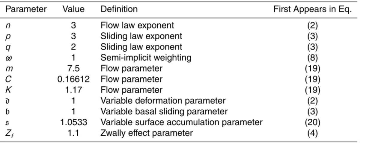
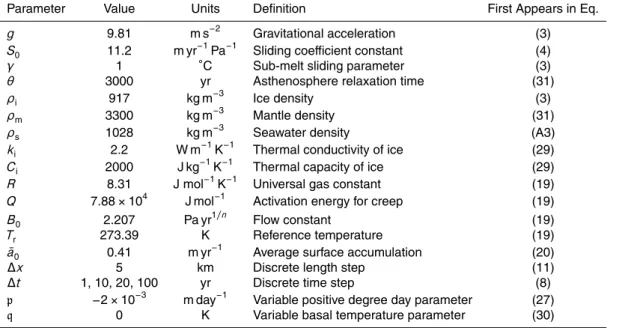
We use a semi-implicit scheme ofω=1, a flow law exponent of n=3, and sliding law

10

exponents ofp=3 and q=2. A list of these non-dimensional parameters and other scaling factors used in the GLISTEN model is given in Table 1, while physical constants and global dimensional parameters are given in Table 2.

3.2 Model parameterizations

In the GLISTEN model, ice flow is thermomechanically coupled to ambient

temper-15

ature, even though temperature is not explicitly calculated within the ice sheet. The background forcing temperatureTf (with units of◦C) describes the anomalous

temper-ature relative to present conditions, and the background sea level forcingHsldescribes

the anomalous sea level rise relative to today. GLISTEN (as well as GRANTISM) de-fines ice temperatureT (with units of K) in terms of the background forcing temperature

20

through an empirical relationship:

T=

(

Tf+263.15 forTf<0

0.5Tf+263.15 forTf≥0

. (18)

2

(12)

TCD

6, 2751–2788, 2012

Title Page

Tables Figures

◭ ◮

Back Close

Full Screen / Esc

Discussion

P

a

per

|

Dis

cussion

P

a

per

|

Discussion

P

a

per

|

Discussio

n

P

a

per

|

This allows us to define the flow parameterA(T) with the empirical expression

A(T)=m

1

B0

n

exp "

3C

(Tr−T)K

−_RTQ

#

, (19)

whereB0is a flow constant,R is the universal gas constant,Qis the activation energy

for creep,Tris a reference temperature, andm,C, andK are flow parameters.

The surface mass balance ˙abetween surface accumulation ˙aaccand surface ablation

5

˙

aablover the ice sheet is defined as ˙a=a˙acc+a˙abl. Surface accumulation in all grid cells

is taken to be the average from regional climate model output (Ettema et al., 2009) along our model flow-line. All precipitation is assumed to fall as snow. This mean value for surface accumulation is constant along the flow-line and represented by ¯a0. Surface

accumulation then can be written as

10

˙

aacc=a¯0×sT ⋆

f_, ₍₂₀₎

wheresis fixed ats=1.0533,T_f⋆=Tf forTf≤0, andTf⋆=0 otherwise.

Mean annual surface temperatures Tma and July mean surface temperatures Tms

are parameterized as functions of altitudeh, latitudeφ, and longitude λaccording to Fausto et al. (2009) so that

15

Tma=41.83−6.309h−0.7189φ+0.0672λ+Tf, and (21)

Tms=14.70−5.426h−0.1585φ+0.0518λ+Tf, (22)

where we specify the latitudeφ=72◦. If we further assume that annual temperature

Tacvaries sinusoidally with timet so that

20

Tac(t)=Tma+(Tms−Tma) cos

2πt

A , (23)

where A=1 yr, then we can calculate the number of positive degree days using the semi-analytic solution developed by Calov and Greve (2005). We first define the

(13)

TCD

6, 2751–2788, 2012

Title Page

Tables Figures

◭ ◮

Back Close

Full Screen / Esc

Discussion

P

a

per

|

Dis

cussion

P

a

per

|

Discussion

P

a

per

|

Discussio

n

P

a

per

|

complementary error function as

erfc(x)=_√2 π

∞ Z

x

exp−x˜2d ˜x (24)

so that the number of positive degree days in one year can be written as

PDD=

A

Z

0

"

σ

√

2πexp −

Tac2

2σ2

!

+Tac

2 erfc

− Tac

σ√2

#

dt, (25)

(Calov and Greve, 2005) whereσis standard deviation of the annual cyclic temperature

5

from the mean annual temperature. We expressσanalytically by applying the definition of standard deviation to Eqs. (21–23) and integrating by parts to result in

σ=

v u u u t 1

A

Z

0

(Tac−Tma)2dt=

Tms−Tma

√

2

, (26)

which accounts for time variation in temperature by noting that∂Tms/∂t=∂Tma/∂t=

dTf/dt (i.e. both Tms and Tma change at the same rate). This parameterization allows

10

us to write surface ablation in terms of PDD and a positive degree day factorpas

˙

a_abl=pPDD, (27)

where the factorpis fixed atp=−2_×10−3m day−1. This simple balance between mass accumulation and loss represents processes such as surface snowfall, surface melting, percolation of meltwater within the ice sheet, and refreezing.

15

Although our simple model cannot explicitly resolve temperature profiles across the entire ice sheet, we can calculate a value for the basal temperatureTb by using Fick’s

(14)

TCD

6, 2751–2788, 2012

Title Page

Tables Figures

◭ ◮

Back Close

Full Screen / Esc

Discussion

P

a

per

|

Dis

cussion

P

a

per

|

Discussion

P

a

per

|

Discussio

n

P

a

per

|

Second Law

∂Tb

∂t =κ ∂2Tb

∂φ2 (28)

to represent thermal di_ffusion in terms of the di_ffusion coe_fficientκ. For ice, we can write

κ= ki ρiCi

, (29)

5

whereki is the thermal conductivity of ice and Ci is the thermal capacity of ice. We

assume that the temperature at the top of the ice sheet is equal to the mean annual temperatureTmain Eq. (21), which allows us to solve for basal temperatureTb(t,φ) as

a function of time and location along the flow-line:

Tb=Tmaerfc

H

2√κt

+q, (30)

10

where the termqrepresents a geothermal energy flux and initially is fixed atq₌0 K. Bedrock deflection follows a relaxation scheme with a time scaleθto determine local isostatic equilibrium:

∂b ∂t =

1

θ

b0−b−

ρi

ρm

H

, (31)

whereρm is the mantle density. Hereb0is the isostatically adjusted bedrock elevation

15

that would result by removing the current load of ice defined as

b0=bobs+

ρi

ρm

Hobs, (32)

wherebobs and Hobs are the bedrock height and ice height used as initial conditions,

respectively. The starting distributions of bedrock topography bobs and ice thickness

(15)

TCD

6, 2751–2788, 2012

Title Page

Tables Figures

◭ ◮

Back Close

Full Screen / Esc

Discussion

P

a

per

|

Dis

cussion

P

a

per

|

Discussion

P

a

per

|

Discussio

n

P

a

per

|

Hobs in these simulations follow a ∆x=36 km resampled grid spacing based on

ob-servations (Letreguilly et al., 1991). We also prevent the ice sheet from expanding into the ocean by specifying an ice thicknessH =0 at the Eastern and Western boundaries whereb < Hslso that the bedrock is beneath sea level.

4 Pre-calibration 5

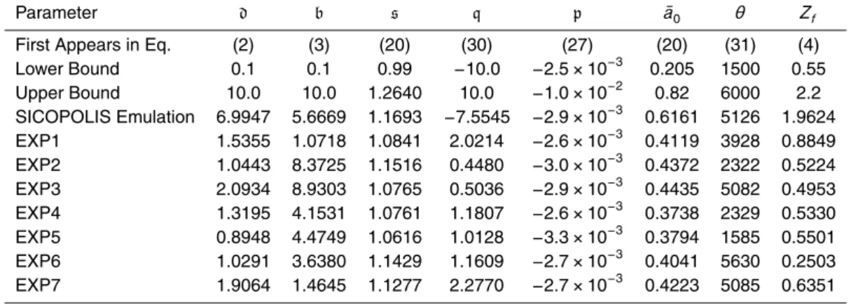
The physical parameterizations described above depend on several uncertain param-eters that can generate substantial variation in model behavior. We perform a pre-calibration of GLISTEN by adjusting the eight variable parameters listed in Table 3 in order to obtain a model that is capable of reproducing geological data and modern ob-servations (Letreguilly et al., 1991; Rignot et al., 2008; Alley et al., 2010). We first use

10

GLISTEN to emulate the behavior of a three-dimensional ice sheet model. We then use this solution as the initial state for a series of seven experiments for pre-calibration according to three possible constraints on GIS behavior (listed in Table 4).

We calculate a score for each model calculation by defining a loss function based on changes in the volume of the GIS∆V (in meters of sea level equivalent) with respect

15

to the present. In general, this loss function is expressed in terms of the mean value

µi and standard deviation σi of theith pre-calibration constraint as a sum over allN

constraints:

L=

N

X

i=0







−log 

 1

σ_i√2πexp



−

∆V_i₋µ_i σ_i√2

!2

 

 





. (33)

The score in Eq. (33) is expressed as a negative logarithm of probability so that model

20

calculations can be compared with one another through minimization and combined as a sum.

We use the differential evolution algorithm (Storn and Price, 1997; Price et al., 2005) to generate a population of model calculations and select an optimal set of parameters.

(16)

TCD

6, 2751–2788, 2012

Title Page

Tables Figures

◭ ◮

Back Close

Full Screen / Esc

Discussion

P

a

per

|

Dis

cussion

P

a

per

|

Discussion

P

a

per

|

Discussio

n

P

a

per

|

Differential evolution (DE) is an iterative genetic algorithm for optimization that takes a parent population of model parameter configurations, forms a mutant population of new configurations, and selects among these candidates for fitness (by minimizing the loss function Eq. 33) to form a new child population. This process is repeated until the DE algorithm reaches a statistically steady state to yield an optimized set of

5

parameters.

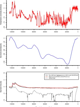
We begin by pre-calibrating GLISTEN so as to emulate the behavior of the SICOPO-LIS three-dimensional ice sheet model. We use the forcing data and volume calcula-tions from run #29 of Applegate et al. (2012), which yields the best match to the esti-mated volume of the modern GIS (Bamber et al., 2001). As constraints, we compare

10

the ice volume of GLISTEN to the SICOPOLIS calculation at three locations along the time series: (1) an average over a warm period in the Eemian (from 118 500 to 115 000 yr ago; the actual timing of the Eemian peak warmth is probably somewhat older, around 125–127 ka, but we use this range here because it is the warmest quasi-Eemian period in the GRIP ice core record); (2) an average during the Last Glacial

15

Maximum (from 20 000 to 19 000 yr ago); and (3) the last time step at present day. All three of these constraints assume a standard deviation of one meter of sea level equivalent volume. We initialize GLISTEN with a present-day GIS profile and force the model using the same temperature forcing Tf, sea level forcing Hsl as the

SICOPO-LIS calculation. The result of this pre-calibration of GSICOPO-LISTEN to SICOPOSICOPO-LIS is shown

20

in Fig. 2, which also shows that the GLISTEN emulation is a significantly better fit to SICOPOLIS than GRANTISM. Although the emulation is not able to precisely replicate the behavior of SICOPOLIS, it follows the major trends and provides a place to begin further pre-calibration experiments.

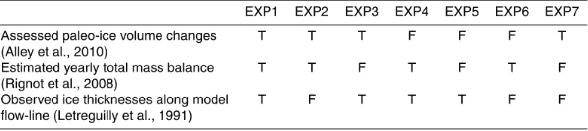
We next define a series of seven pre-calibration experiments that are defined

ac-25

cording to the combinations of three sets of constraints from data. The first constraint is based on expert assessment of GIS volume changes at different times in the past (Alley et al., 2011) and provides a range for sea level rise from Greenland ice during the Eemian, the Last Glacial Maximum, and present day. These paleo-constraints are

(17)

TCD

6, 2751–2788, 2012

Title Page

Tables Figures

◭ ◮

Back Close

Full Screen / Esc

Discussion

P

a

per

|

Dis

cussion

P

a

per

|

Discussion

P

a

per

|

Discussio

n

P

a

per

|

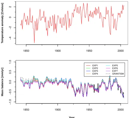
shown as grey boxes in Fig. 3, where the width of the box is the time period consid-ered and the height of the box is the range of sea level rise (see Alley et al., 2010). The second constraint is based on instrumental data (Rignot et al., 2008) from recent decades of the mass balance of the GIS. These five constraints are shown as grey bars in Fig. 4, where the height of the bar is one standard deviation for mass balance.

5

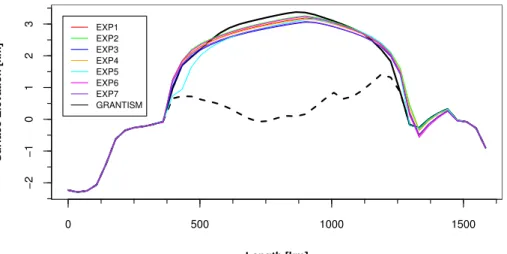
The third constraint is based on the similarity of the calculated ice sheet profile to the observed GIS profile; we use the parameter estimation method described by Olson et al. (2012) as the loss function for this constraint. The constraint on the GIS profile is shown as the solid black line in Fig. 5, which is the present-day geography interpo-lated to a∆x=36 km grid. The combinations of these three constraints yield the seven

10

experiments that are outlined in Table 4.

We initialize the model with a present-day GIS profile and use a temperature forcing

Tf and sea level forcing Hsl from GRIP, the Greenland Ice Core Project (Dansgaard

et al., 1993; Johnsen et al., 1997; shown in the top two panels of Fig. 2), with a timestep

∆t=100 yr. The best fits to the data sets considered in experiments EXP1 through

15

EXP7 are shown in Fig. 3 as sea level rise due to changes in the GIS over the past 125 000 yr. The seven model configurations show varied behavior with time, although they all stay within range of the three paleo-constraints on sea level rise. It is interesting to note that even the experiments that do not consider the paleo-constraints (EXP4, EXP5, and EXP6) still behave similarly to the other configurations. The seven GLISTEN

20

experiments, however, provide geologically consistent trajectories for GIS volume that show a more dynamic response than the original GRANTISM implementation.

We then continue integrating the GLISTEN model using temperature forcingTf from

instrumental records over the past 150 yr (Vinther et al., 2006), a constant sea level

Hsl=0, and a timestep ∆t=1 yr. The optimal parameter configurations for EXP1

25

through EXP7 are shown in Fig. 4 as the GIS mass balance over the past 150 yr. All these experiments show a close agreement to one another and fall within one stan-dard deviation of the instrumental data constraints. Three of these pre-calibration ex-periments (EXP3, EXP5, and EXP7) did not consider the constraints from instrumental

(18)

TCD

6, 2751–2788, 2012

Title Page

Tables Figures

◭ ◮

Back Close

Full Screen / Esc

Discussion

P

a

per

|

Dis

cussion

P

a

per

|

Discussion

P

a

per

|

Discussio

n

P

a

per

|

data, yet even these calculations show agreement with recent records. GLISTEN ap-pears to accurately represent the recent instrumental record using a variety of param-eter configurations.

Upon completing this pre-calibration, the final GIS profile for the seven experiments is shown in Fig. 5. All seven profiles are similar to one another, including the three

5

experiments (EXP2, EXP6, and EXP7) that did not consider the constraint on the final GIS profile. The optimal parameter configurations for EXP1 through EXP7 are given in Table 3, which includes the prior ranges of each parameter and the SICOPOLIS em-ulation. All of these model configurations show a range in parameter values, although almost none of them approach the lower or upper prior ranges. These experiments

10

(EXP1 through EXP7, plus the SICOPOLIS emulation) describe eight potential ways to configure the parameters in GLISTEN.

5 Discussion

The pre-calibration experiments described above provide several potential ways to con-figure the GLISTEN model. These model configurations compare with results from the

15

three-dimensional ice sheet model SICOPOLIS and satisfy constraints based on as-sessed paleo-ice volume changes and instrumental records. For these reasons, GLIS-TEN may be useful as a tool to model the behavior of the GIS during time periods from the Eemian to the present.

GLISTEN’s advantage over three-dimensional models is that it features much shorter

20

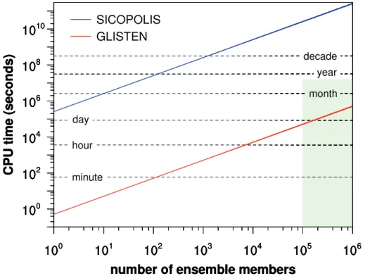
computation time. We illustrate this in Fig. 6, which shows the CPU time required to compute a 125 000 yr paleo-calculation, for which GLISTEN takes about half a second and SICOPOLIS takes a few days. The computational speed of GLISTEN makes it an ideal tool for use in IAMs. Simulations with IAMs often use large numbers of en-semble members (>105) in order to consider a wide range of possibilities for climate

25

change and therefore require a reasonable timescale (<6 months) for computation (e.g. McInerney and Keller, 2008; Goes et al., 2011; McInerney et al., 2011), shown as the

(19)

TCD

6, 2751–2788, 2012

Title Page

Tables Figures

◭ ◮

Back Close

Full Screen / Esc

Discussion

P

a

per

|

Dis

cussion

P

a

per

|

Discussion

P

a

per

|

Discussio

n

P

a

per

|

green shaded area in Fig. 6. For such ensemble sizes, GLISTEN would require weeks to months of CPU time, whereas SICOPOLIS would require decades or more to per-form the same calculations. In this case, one-dimensional flow-line models are a more practical tool than more complex models. The behavior of the GIS is relevant for IAMs because changes in the volume of the GIS contribute to changes in sea level. Although

5

three-dimensional ice sheet models would be far too time consuming, GLISTEN pro-vides a rapid way to simulate GIS behavior for use in IAMs and other applications.

In summary, the full GLISTEN model is able to reproduce historical trends in the GIS from ice core and instrumental data. This model is simplified relative to three-dimensional models, such as SICOPOLIS, but it provides the advantage of rapid

com-10

putational speed.

6 Conclusions

The GLISTEN one-dimensional flow-line model provides a computationally efficient tool for calculating changes in the GIS over the past 125 000 yr and can be configured using several sets of observational constraints and, consequently, several parameter

15

configurations. The GLISTEN model can compute changes in the GIS at several orders of magnitude faster than three-dimensional ice sheet models. This makes GLISTEN an ideal candidate for implementation into IAMs to incorporate the dependence of GIS changes on sea level. In future work we will perform a full calibration of GLISTEN and incorporate it as a module in an IAM.

20

Appendix A

Changes from GRANTISM

GLISTEN is a direct descendent of GRANTISM by Pattyn (2006), and most of the basic equations and numerical methods are identical between the two models. Nearly

(20)

TCD

6, 2751–2788, 2012

Title Page

Tables Figures

◭ ◮

Back Close

Full Screen / Esc

Discussion

P

a

per

|

Dis

cussion

P

a

per

|

Discussion

P

a

per

|

Discussio

n

P

a

per

|

all parameters are identical between GLISTEN and GRANTISM, as well (with the one exception that GRANTISM uses a value ofρi=910 kg m−

3

for the density of ice). We have, however, made several changes to physical parameterizations in the model that differ from those used in GRANTISM. In particular, the representation of mass balance in GLISTEN is analytically defined in terms of the number of positive degree days

5

at a particular location along the GIS flow-line, which is a substantial improvement upon the simplified parameterization used in GRANTISM. GLISTEN also implements an improved representation of basal sliding, which includes the “Zwally effect”, and basal temperature. Below we describe the specific components of GRANTISM that differ from those in GLISTEN.

10

The expression for basal sliding in GRANTISM di_ffers from that in the GLISTEN implementation (c.f. Eq. 3) and can be written as

u(b)=Ab

τ_dp

Z⋆, (A1)

whereAbis related to the flow parameter as

Ab=

1

2A(T)×10

6_. _(A2)

15

HereZ⋆is the height of the ice above surface buoyancyZ⋆, which is defined as

Z⋆=H+ρ_ρs

i

min

(b−Hsl) , 0

, (A3)

whereρs is the density of seawater. The eustatic sea level Hsl is also prescribed in

GRANTISM as a function ofTfand with maximum lower bound so that

Hsl=max{min [15Tf, 0] ,−150}. (A4)

20

(21)

TCD

6, 2751–2788, 2012

Title Page

Tables Figures

◭ ◮

Back Close

Full Screen / Esc

Discussion

P

a

per

|

Dis

cussion

P

a

per

|

Discussion

P

a

per

|

Discussio

n

P

a

per

|

The representation of mass balance in GRANTISM also differs from the mass balance scheme used by GLISTEN. Surface accumulation in GRANTISM follows a second-order polynomial fit by Pattyn (2006) to the data of Ohmura and Reeh (1991) as

˙

aacc=

−2.46257+0.1367λ−0.0016λ2×1.0533Tf⋆_, _(A5)

with units of m yr−1ice equivalent (c.f. Eq. 20). Additionally, the form of the mean

sum-5

mer surface temperature (Eq. 22) di_ffers in GRANTISM and is parameterized as

Tms=−7.2936−0.006277h+Tf. (A6)

(Note that Eq. 15 of Pattyn, 2006, takes a slightly truncated form withTms=−7.29−

0.006277h+T_f, although the full equation above appears in the code for GRANTISM.) Surface ablation in GRANTISM likewise takes a simpler form than Eq. (27) because

10

it is only dependent on Tms and not on an annual cycle. The expression for surface

ablation in GRANTISM follows

˙

aabl=

(

max

−1.4T_ms,₋10

forT_ms_≥0

0 forTms<0

, (A7)

where a minimum ablation limit of₋10 m yr−1is imposed (c.f. Eq. 27).

GRANTISM predicts significantly larger growth of the GIS over the past 125 000 yr in

15

Fig. 3 when compared to any of our pre-calibration experiments or to SICOPOLIS. This suggests that GRANTISM may be limited in its ability to simulate dynamic responses to the GIS over geologic timescales. GRANTISM is more accurate at representing recent perturbations in the GIS, as shown by the similarity between GRANTISM and the seven pre-calibration curves in Fig. 4. This suggests to us that GRANTISM may be a useful

20

tool for modeling recent changes in temperature.

(22)

TCD

6, 2751–2788, 2012

Title Page

Tables Figures

◭ ◮

Back Close

Full Screen / Esc

Discussion

P

a

per

|

Dis

cussion

P

a

per

|

Discussion

P

a

per

|

Discussio

n

P

a

per

|

Acknowledgements. We thank Roman Olson for his assistance with parameter estimation for the ice sheet profile. This research was supported in part by the US Department of Energy, Office of Science, Biological and Environmental Research Program, Integrated Assessment Program, through Grant No. DE-SC0005171, as well as the Penn State Center for Climate Risk Management. All errors and opinions are our own.

5

References

Alley, R. B.: Continuity comes first: recent progress in understanding subglacial deformation, in: Deformation of Glacial Materials, edited by: Maltman, A. J., Hubbard, B., and Hambrey, M. J., Geol. Soc. Spec. Publ., 176, 171–179, 2000.

Alley, R. B., Horgan, H. J., Joughin, I., Cuffey, K. M., Dupont, T. K., Parizek, B. R.,

Anan-10

dakrishnan, S., and Bassis, J.: A simple law for ice-shelf calving, Science, 322, 1344, doi:10.1126/science.1162543, 2008.

Alley, R. B., Andrews, J. T., Brigham-Grette, J., Clarke, G. K. C., Cuffey, K. M., Fitzpatrick, J. J., Funder, S., Marshall, S. J., Miller, G. H., Mitrovica, J. X., Muhs, D. R., Otto-Bliesner, B. L., Polyak, L., and White, J. W. C.: History of the Greenland ice sheet: paleoclimate insights,

15

Quaternary Sci. Rev., 29, 1728–1756, 2010.

Applegate, P. J., Kirchner, N., Stone, E. J., Keller, K., and Greve, R.: An assessment of key model parametric uncertainties in projections of Greenland Ice Sheet behavior, The Cryosphere, 6, 589–606, doi:10.5194/tc-6-589-2012, 2012.

Bales, R. C., Guo, Q., Shen, D., McConnell, J. R., Guoming, D., Burkhart, J. F., Spikes, V. B.,

20

Hanna, E., and Cappelen, J.: Annual accumulation for Greenland updated using ice core data developed during 2000–2006 and analysis of daily coastal meteorological data, J. Geophys. Res., 114, D06116, doi:10.1029/2008JD011208, 2009.

Bamber, J. L., Layberry, R. L., and Gogineni, S. P.: A new ice thickness and bed data set for the Greenland ice sheet, 1. Measurement, data reduction, and errors, J. Geophys. Res., 106,

25

33773–33780, 2001.

Bartholomew, I., Nienow, P., Mair, D., Hubbard, A., King, M. A., and Sole, A.: Seasonal evolution of subglacial drainage and acceleration in a Greenland outlet glacier, Nat. Geosci., 3, 408– 411, 2010.

(23)

TCD

6, 2751–2788, 2012

Title Page

Tables Figures

◭ ◮

Back Close

Full Screen / Esc

Discussion

P

a

per

|

Dis

cussion

P

a

per

|

Discussion

P

a

per

|

Discussio

n

P

a

per

|

Braithwaite, R. J.: Positive degree-day factors for ablation on the Greenland ice sheet studied by energy-balance modelling, J. Glaciol., 41, 153–160, 1995.

Bueler, E. and Brown, J.: Shallow shelf approximation as a “sliding law” in a thermomechanically coupled ice sheet model, J. Geophys. Res., 114, F03008, doi:10.1029/2008JF001179, 2009. Calov, R. and Greve, R.: A semi-analytical solution for the positive degree-day model with

5

stochastic temperature variations, J. Glaciol., 51, 173–175, 2005.

Calov, R. and Marsiat, I.: Simulations of the Northern Hemisphere through the last glacial-interglacial cycle with a vertically integrated and a 3-D thermomechanical ice sheet model coupled to a climate model, Ann. Glaciol., 27, 169–176, 1998.

Cane, M. A. and Zebiak, S. E.: A theory for El Ni ˜no and the southern oscillation, Science, 228,

10

1085–1087, 1985.

Cuffey, K. M. and Clow, G. D.: Temperature, accumulation, and ice sheet elevation in Central Greenland through the last deglacial transition, J. Geophys. Res., 102, 26383–26396, 1997. Cu_ffey, K. M. and Kavanaugh, J. L.: How nonlinear is the creep deformation of polar ice? A new

field assessment, Geology, 39, 1027–1030, 2011.

15

Dahl-Jensen, D. and Gundestrup, N. S.: Constitutive properties of ice at Dye-3, Greenland, in: The Physical Basis of Ice Sheet Modelling, edfited by: Waddington, E. and Walder, J., IAHS-AISH P., 170, 31–43, 1987.

Dansgaard, W., Johnsen, S., Clausen, H., Dahl-Jensen, D., Gundestrup, N., Hammer, C., Hvid-berg, C., Steffensen, J., Sveinbjornsdottir, A., and Jouzel, J.: Evidence for general instability

20

of past climate from a 250-kyr ice-core record, Nature, 364, 218–220, 1993.

Dupont, T. K. and Alley, R. B.: Assessment of the importance of shelf buttressing to ice-sheet flow, Geophys. Res. Lett., 32, L0450, doi:10.1029/2004GL022024, 2005.

Ekholm, S.: A full coverage, high-resolution, topographic model of Greenland computed from a variety of digital elevation data, J. Geophys. Res., 101, 21961–21972, 1996.

25

Fausto, R. S., Ahlstrom, A. P., van As, D., Boggild, C. E., and Johnsen, S. J.: A new present-day temperature parameterization for Greenland, J. Glaciol., 55, 95–105, 2009.

Glen, J. W.: The creep of polycrystalline ice, P. R. Soc. Lond. A, 228, 519–538, doi:10.1098/rspa.1955.0066, 1955.

Goes, M., Keller, K., and Tuana, N.: The economics (or lack thereof) of aerosol geoengineering,

30

Climatic Change, 109, 719–744, 2011.

Goldsby, D. L. and Kohlstedt, D. L.: Superplastic deformation of ice: experimental observa-tions, J. Geophys. Res., 106, 11017–11030, 2001.

(24)

TCD

6, 2751–2788, 2012

Title Page

Tables Figures

◭ ◮

Back Close

Full Screen / Esc

Discussion

P

a

per

|

Dis

cussion

P

a

per

|

Discussion

P

a

per

|

Discussio

n

P

a

per

|

Greve, R.: Application of a polythermal three-dimensional ice sheet model to the Greenland ice sheet: response to steady-state and transient climate scenarios, J. Climate, 10, 901–918, 1997.

Greve, R.: On the response of the Greenland ice sheet to greenhouse climate change, Climatic Change, 46, 289–303, 2000.

5

Greve, R.: Relation of basal measured temperatures and the spatial distribution of the geother-mal heat flux for the Greenland Ice Sheet, Ann. Glaciol., 42, 424–432, 2005.

Greve, R. and Blatter, H.: Dynamics of Ice Sheets and Glaciers, Monograph Series Advances in Geophysical and Environmental Mechanics and Mathematics, 2009.

Greve, R. and Otsu, S.: The effect of the north-east ice stream on the Greenland ice sheet in

10

changing climates, The Cryosphere Discuss., 1, 41–76, doi:10.5194/tcd-1-41-2007, 2007. Greve, R., Saito, F., and Abe-Ouchi, A.: Initial results of the SeaRISE numerical experiments

with the models SICOPOLIS and IcIES for the Greenland ice sheet, Ann. Glaciol., 52, 23–30, 2011.

Hindmarsh, R. C. A. and Le Meur, E.: Dynamical processes involved in the retreat of marine

15

ice sheets, J. Glaciol., 47, 271–279, 2001.

Hulme, M., Raper, S. C. B., and Wigley, T. M. L.: An integrated framework to address climate change (ESCAPE) and further developments of the global and regional climate modules (MAGICC), Energ. Policy, 23, 347–355, 1995.

Hutter, K.: Theoretical Glaciology: Material Science of Ice and the Mechanics of Glaciers and

20

Ice Sheets, D. Reidel, Dordrecht, 1983.

Huybrechts, P. and de Wolde, J.: The dynamic response of the Greenland and Antarctic ice sheets to multiple-century climatic warming, J. Climate, 12, 2169–2188, 1999.

Johnsen, S., Clausen, H., Dansgaard, W., Gundestrup, N., Hammer, C., Andersen, U., An-dersen, K., Hvidberg, C., Dahl-Jensen, D., and Steffensen, J.: Theδ18O record along the

25

Greenland Ice Core Project deep ice core and the problem of possible Eemian climatic in-stability, J. Geophys. Res., 102, 26397–26410, 1997.

Keller, K., Deutsch, C., Hall, M. G., and Bradford, D. F.: Early detection of changes in the North Atlantic meridional overturning circulation: implications for the design of ocean observation systems, J. Climate, 20, 145–157, 2007.

30

Kirchner, N., Hutter, K., Jakobsson, M., and Gyllencreutz, R.: Capabilities and limitations of numerical ice sheet models: a discussion for Earth-scientists and modelers, Quaternary Sci. Rev., 30, 3691–3704, 2011.

(25)

TCD

6, 2751–2788, 2012

Title Page

Tables Figures

◭ ◮

Back Close

Full Screen / Esc

Discussion

P

a

per

|

Dis

cussion

P

a

per

|

Discussion

P

a

per

|

Discussio

n

P

a

per

|

Larour, E., Seroussi, H., Morlighem, M., and Rignot, E.: Continental scale, high order, high spatial resolution ice sheet modeling using the Ice Sheet System Model (ISSM), J. Geophys. Res., 17, F01022, doi:10.1029/2011JF002140, 2012.

Leng, W., Ju, L., Gunzburger, M., Price, S., and Ringler, T.: A parallel high-order accurate finite element nonlinear Stokes ice sheet model and benchmark experiments, J. Geophys. Res.,

5

117, F01001, doi:10.1029/2011JF001962, 2012.

Letreguilly, A., Huybrechts, P., and Reeh, N.: Steady-state characteristics of the Greenland ice sheet under different climates, J. Glaciol., 37, 149–157, 1991.

Lhomme, N., Clarke, G. K. C., and Marshall, S. J.: Tracer transport in the Greenland ice sheet: constraints on ice cores and glacial history, Quaternary Sci. Rev., 24, 173–194, 2005.

10

Lunt, D. J., de Noblet-Ducoudre, N., and Charbit, S.: Effects of a melted Greenland ice sheet on climate, vegetation, and the cryosphere, Clim. Dynam., 23, 679–694, 2004.

Lythe, M. B., Vaughan, D. G., and the Bedmap Consortium: Bedmap: a new ice thickness and subglacial topography model of Antarctica, J. Geophys. Res., 106, 11335–11351, 2001. MacAyeal, D. M.: Large-scale ice flow over a viscous basal sediment: theory and application to

15

Ice Stream B, Antarctica, J. Geophys. Res., 94, 4071–4087, 1989.

Marsiat, I.: Simulation of the Northern Hemisphere continental ice sheets over the last glacial-interglacial cycle: experiments with a latitude-longitude vertically integrated ice sheet model coupled to a zonally averaged climate model, Palaeoclimates, 1, 59–98, 1994.

McInerney, D. and Keller, K.: Economically optimal risk reduction strategies in the face of

un-20

certain climate thresholds, Climatic Change, 91, 29–41, 2008.

McInerney, D., Lempert, R., and Keller, K.: What are robust strategies in the face of uncertain cli-mate threshold responses?, Climatic Change, 112, 547–568, doi:10.1007/s10584-011-0377-1, 2011

Meehl, G. A., Stocker, T. F., Collins, W. D., Friedlingstein, A. T., Gaye, A. T., Gregory, J. M.,

25

Kitoh, A., Knutti, R., Murphy, J. M., and Noda, A.: Global climate projections, in: Climate Change 2007: The Physical Science Basis. Contribution of Working Group I to the Fourth As-sessment Report of the Intergovernmental Panel on Climate Change, edited by: Solomon, S., Qin, D., Manning, M., Chen, Z., Marquis, M., Averyt, K. B., Tignor, M., and Miller, H. L., Cam-bridge University Press, 2007.

30

Mote, T. L.: Greenland surface melt trends 1973–2007: evidence of a large increase in 2007, Geophys. Res. Lett., 34, L22507, doi:10.1029/2007GL031976, 2007.

(26)

TCD

6, 2751–2788, 2012

Title Page

Tables Figures

◭ ◮

Back Close

Full Screen / Esc

Discussion

P

a

per

|

Dis

cussion

P

a

per

|

Discussion

P

a

per

|

Discussio

n

P

a

per

|

Nye, J. F.: The distribution of stress and velocity in glaciers and ice-sheets, P. R. Soc. Lond. A, 239, 113–133, doi:10.1098/rspa.1957.0026, 1957.

Olson, R., Sriver, R., Goes, M., Urban, N. M., Matthews, H. D., Haran, M., and Keller, K.: A climate sensitivity estimate using Bayesian fusion of instrumental observations and an Earth System model, J. Geophys. Res., 117, D04103, doi:10.1029/2011JD016620, 2012.

5

Parizek, B. R. and Alley, R. B.: Implications of increased Greenland surface melt under global-warming scenarios: ice sheet simulations, Quaternary Sci. Rev., 23, 1013–1027, 2004. Paterson, W. S. B. and Budd, W. F.: Flow parameters for ice sheet modeling, Cold Reg. Sci.

Technol., 6, 175–177, 1982.

Pattyn, F.: GRANTISM: an Excel(TM) model for Greenland and Antarctic ice-sheet response to

10

climate changes, Comput. Geosci., 32, 316–325, 2006.

Peltier, W. R.: Global glacial isostasy and the surface of the ice-age Earth: the ICE-5G (VM2) model and GRACE, Annu. Rev. Earth Pl. Sc., 32, 111–149, 2004.

Pollard, D. and DeConto, R. M.: Antarctic ice and sediment flux in the Oligocene simulated by a climate-ice sheet-sediment model, Palaeogeogr. Palaeocl., 198, 53–67, 2003.

15

Pollard, D. and DeConto, R.: Modelling West Antarctic ice sheet growth and collapse through the past five million years, Nature, 458, 329–333, 2009.

Press, W. H., Teukolsky, S. A., Vetterling, W. T., and Flannery, B. P.: Numerical Recipes: The Art of Scientific Computing, 3rd edn., Cambridge University Press, 2007.

Price, K. V., Storn, R. M., and Lampinen, J. A.: Differential evolution: a practical approach to

20

global optimization, Springer-Verlag, New York, 2005.

Price, S. F., Payne, A. J., Howat, I. M., and Smith, B. E.: Committed sea-level rise for the next century from Greenland ice sheet dynamics during the past decade, P. Natl. Acad. Sci. USA, 108, 8978–8983, 2011.

Reeh, N.: Parameterization of melt rate and surface temperature on the Greenland ice sheet,

25

Polarforschung, 59, 113–128, 1898.

Rignot, E., Box, J., Burgess, E., and Hanna, E.: Mass balance of the Greenland ice sheet from 1958 to 2007, Geophys. Res. Lett., 35, L20502, doi:10.1029/2008GL035417, 2008.

Robinson, A., Calov, R., and Ganopolski, A.: An e_fficient regional energy-moisture bal-ance model for simulation of the Greenland Ice Sheet response to climate change, The

30

Cryosphere, 4, 129–144, doi:10.5194/tc-4-129-2010, 2010.