ESTIMATION OF GENETIC PARAMETERS IN THE ANALYSIS OF SQUARE LATTICE EXPERIMENT GROUP

(1)

ESTIMATION OF GENETIC PARAMETERS IN THE ANALYSIS OF SQUARE LATTICE... 195

Bragantia, Campinas, 58(1):195-208, 1999

ESTIMATION OF GENETIC PARAMETERS

IN THE ANALYSIS OF SQUARE LATTICE

EXPERIMENT GROUP

(1)

JOSÉ MARCELO SORIANO VIANA (2)_{& ADAIR JOSÉ REGAZZI}(3)

ABSTRACT

Aiming to demonstrate how to obtain unbiased estimates of genetic parameters of base populations, unaffected by genotype x environment effects, this paper presents the vari-ance and covarivari-ance components of the intra-block analysis of a group of square lattice experiments and the estimators of the components associated to treatment effect. Random model and mixed models with environment effect fixed and other effects random are consid-ered. In the analysis with treatments not corrected for blocks/replications/environments, the estimators of the variance and covariance components due to treatment effect are different from those of the analysis considering the complete block model. Data from two experi-ments of a breeding program of Eucalyptus pyrocarpa were used for genetic analysis. The

analysis of variance of height and diameter indicated absence of interaction between prog-eny and environment. Due to this result, the prediction of the direct and indirect genetic gains was based on the mean of the two environments. The high estimates of narrow sense heritabilities and additive genetic correlation indicate that selection of the superior families will be effective in changing the means of the base population for both traits.

Index terms: quantitative genetics, genetic parameters, variance components, covariance

components, joint analysis, square lattice.

(1)_{Received for publication in April 23, 1997, and approved in December 9, 1998.}

(2)

RESUMO

ESTIMAÇÃO DE PARÂMETROS GENÉTICOS NA ANÁLISE DE GRUPO DE EXPERIMENTOS EM LÁTICE QUADRADO

Neste trabalho, discute-se a estimação de parâmetros genéticos de populações-base, quando as famílias amostradas foram avaliadas em dois ou mais ambientes, no delineamento em látice quadrado. Na parte teórica, são apresentados os componentes de variância e covariância da análise intrablocos de grupo de experimentos em látice quadrado e os estimadores dos componentes associados a efeito de tratamento, considerando estimação pelo método dos quadrados mínimos ordinário. Os estimadores dos componentes da variância e covariância da análise com tratamentos não ajustados diferem dos da análise segundo mode-lo em bmode-locos completos. Além de modemode-lo aleatório, consideram-se também os mistos com efeito de ambiente fixo e demais efeitos aleatórios. Dados de dois experimentos de um pro-grama de melhoramento de Eucalyptus pyrocarpa foram usados para análise genética. Como

em relação às características altura e diâmetro não houve evidência de interação progênie x ambiente, a predição de ganhos diretos e indiretos foi feita com base na média dos dois ambientes. Os valores elevados da herdabilidade em sentido restrito e da correlação genética aditiva evidenciam que a seleção das famílias superiores será eficiente em alterar as médias da população-base, para as duas características.

Termos de indexação: genética quantitativa, parâmetros genéticos, componentes da variância,

componentes da covariância, análise conjunta, látice quadrado.

1. INTRODUCTION

The evaluation of a group of treatments (fami-lies, varieties etc.) in more than one environmental condition is common in breeding programs. This al-lows to study the interaction between treatments and environments (local and/or years, and so on) and, when the treatments are families sampled from a base popu-lation, the estimation of genetic parameters not af-fected by the progeny x environment interaction. Due to its implication on the selective process by decreas-ing the correlation between phenotypic and genotypic values, the genotype x environment interaction is a complex and widely investigated problem, which must be considered in breeding programs. Since a high number of treatments is normally used in these ex-periments, the lattice design has been frequently used (Zuber, 1942; Johnson & Murphy, 1943; Torrie et al., 1943; Wellhausen, 1943; Bancroft & Smith, 1949; Sahagun-Castellanos & Frey, 1990; Beninati & Busch, 1992; Chaves & Miranda Filho, 1992; Singh et al, 1992; Arriel et al., 1993; Lin et al., 1993; Michelini

& Hallauer, 1993; Moncada et al., 1993; Oliveira, 1993; Ferrão et al., 1994, and Rezende & Ramalho, 1994), contributing to increase experimental error control efficiency (Cochran & Cox, 1957, and Federer, 1955).

In many cases, however, the joint analysis of lattice experiments and, particularly, the estimation of the variance and covariance components used to estimate genetic parameters, e.g., genotypic variance between families, additive genetic variance, heritabil-ity on a family mean basis, genotypic correlation and expected genetic gain (Kempthorne, 1957), involve approximate processes. The lattice design sometimes is not taken into account with the complete block model being considered.

An exact estimation of the variance and cova-riance components is possible if the expected mean squares are known or if the program used for the analy-sis makes itself the estimation (for example, the VARCOMP procedure of SAS/STAT®_{(SAS Institute,}

(3)

estimates of the variance and covariance components of the intra-block analysis of a group of square lattice experiments, considering the least squares method.

2. THE INTRA-BLOCK ANALYSIS OF A GROUP OF SQUARE LATTICE

EXPERIMENTS

The complete statistical model is:

Y_il(j)(g) = µ + t_i + (r|a)_j(g) + (b|r|a)_l(j)(g) + a_g + (ta)_ig + e_il(j)(g)

where:

Y_il(j)(g) is the observation of the treatment i (i = 1,..., v = k2_{) in the block l (l = 1,..., k) of the replication j (j =}

1,..., m), in the environment g (g = 1,..., s); µ is a constant common to all observations; t_i is the effect of the treatment i;

(r|a)_j(g) is the effect of the replication j in the environ-ment g;

(b|r|a)_l(j)(g) is the effect of the block l of the replication j, in the environment g;

a_g is the effect of the environment g;

(ta)_ig is the effect of the interaction between the treat-ment i and the environtreat-ment g;

e_il(j)(g) is the error associated to the observation Y_il(j)(g) ; e_il(j)(g) ~ N(0, σ2_{), independent.}

The matricial form of the linear model we con-sider is:

Y = XΘ + e; ε ~ N(Φ, σ2_I)

with:

Q’ = [µ | t₁ ... t_v| (r|a)₁₍₁₎ ... (r|a)_m(s) | (b|r|a)_1(1)(1) ... (b|r|a)_k(m)(s) | a₁ ... a_s | (ta)₁₁ ... (ta)_vs]

= [µ | τ’ | α’ | ß’ | δ’ | τδ’]

In the analyses of variance the orthogonal par-titions of the reduction in the total sum of squares due to fitting the complete model will be as follows: R(µ,τ, α, ß, δ, τδ) = R(µ) + R(δ|µ) + R(α|µ, δ) + R(ß|µ,

where R(.) = Y’X(X’X)G_{X’Y is the reduction in the}

total sum of squares due to fitting a certain model, with rank of X(X’X)G_{X’ = rank of X degrees of}

free-dom, being (X’X)G_{any generalized inverse of X’X,}

and R(.|.) is a difference between two R(.) terms (Searle, 1971, 1992, and Graybill, 1976).

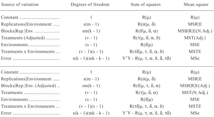
The analyses of variance related to the two par-titions of R(µ, τ, α, ß, δ, τδ) are shown in Table 1.

2.1. The intra-block analysis of random model

The assumptions of the statistical model are: a) t_i ~ N(0, σ2

t), independent;

b) (r|a)_j(g) ~ N(0, σ2

r), independent;

c) (b|r|a)_l(j)(g) ~ N(0, σ2

b), independent;

d) a_g ~ N(0, σ2

a), independent;

e) (ta)_ig ~ N(0, σ2

ta), independent;

f) e_il(j)(g) ~ N(0, σ2_{), independent;}

g) t_i, (r|a)_j(g), (b|r|a)_l(j)(g), a_g, (ta)_ig and e_il(j)(g) are independent.

In the covariance matrix of Y, Cov(Y) = E{[Y -E(Y)][Y - E(Y)]’} = Σ_(n) • σ2_{I, n = smk}2_{, the elements}

are:

V(Y_il(j)(g)) = σ2 t + σ

2 r + σ

2 b +σ

2 a +σ

2 ta +σ

2_{= C} 0

Cov(Y_il(j)(g), Y_i’l(j)(g)) = σ2

r + σ2b + σ2a = C1 (i • i’)

Cov(Y_il(j)(g), Y_{i’l’(j)(g)}) = σ2

r + σ2a = C2 (i • i’ and l • l’)

Cov(Y_il(j)(g),Y_{il’(j’)(g)}) = σ2

t + σ2a + σ2ta = C3 (j • j’)

Cov(Y_il(j)(g), Y_{i’l’(j’)(g)}) = σ2

a = C4 (i • i’ and j • j’)

Cov(Y_il(j)(g), Y_{il’(j’)(g’)}) = σ2

t = C5 (g • g’)

Cov(Y_il(j)(g), Y_{i’l’(j’)(g’)}) = 0 = C₆ (i • i’ and g • g’) Using the property of mathematical expecta-tion of quadratic forms (Searle, 1971, Searle et al. 1992, and Graybill, 1976), the expected values below and those presented in Table 2 can be demonstrated: E(Y’Y) = nµ2_{+ n}_σ2

t+ nσ2r+ nσ2b+ nσ2a+ nσ2ta+ nσ2

E[R(µ)] = nµ2_{+ ms}σ2

t+ vσ2r+ kσ2b+ mvσ2a+ mσ2ta+ σ2

E[R(µ, τ, δ, α, ß)] = nµ2_{+ n}σ2

t+ nσ2r+ nσ2b+ nσ2a +

[mks + mk (k - 1)]σ2

ta + (v + mks - 1)σ2

Considering that the treatments are families sampled from a base population, the two estimators of the vari-ance of the genotypic means of the progenies that can be obtained from the reference population (σ2

(4)

k + 1

k

[

]

(

)

MST (Adj.) - MSTEms

MST(N.Adj.) - MSe - mσ2 ta

k

k + 1

(

)

σ2b(2)

≠

ms

[

]

MST (N. Adj.) - MSTE_CB ms

k + 1

k

(

)

MSTE - MSe_m

σ2 ta =

k(ms - 1) ms

[

MSBR E (Adj.) - MSe -

s - 1

s

(

)

σ2 ta ^ ^

^ ^

σ2 b(2)= ^

(a) t_i = (t_iY + t_iX) ~ (0, σ2

t = σ2tY + σ2tX + 2σtYX), inde-p pendent;

(b) (r|a)_j(g) = [(r|a)_j(g)Y + (r|a)_j(g)X] ~ (0, σ2

r = σ2rY + σ2rX + + 2σrYX), independent;

(c) (b|r|a)_l(j)(g) = [(b|r|a)_l(j)(g)Y + (b|r|a)_l(j)(g)X] ~ (0, σ2 b = = = σ2

bY + σ2bX + 2σbYX), independent;

(d) a_g = (a_gY + a_gX) ~ (0, σ2

a = σ2aY + σ2aX + 2σaYX), i independent;

(e) (ta)_ig = [(ta)_igY + (ta)_igX] ~ (0, σ2

ta = σ2taY + σ2taX +

2σtaYX), independent;

(f) e_il(j)(g) = [e_il(j)(g)Y + e_il(j)(g)X] ~ (0, σ2₌_σ2

Y + σ2X + + + 2σYX), independent;

(g) t_i, (r|a)_j(g), (b|r|a)_l(j)(g), a_g, (ta)_ig and e_il(j)(g) are inde-pendent.

From previous results, the expected mean squares presented in Table 3 are obtained. The two estimators of the covariance between genotypic means of the same family, in relation to Y and X (σ_tYX), are: and MSTE_CB is the treatments x environments

inter-action mean square, considering the complete block model.

Therefore, σ2

t(2) is not the estimator of σ 2

t of

the analysis according to the complete block model. The following statistical models are considered to estimate covariance components:

Y_il(j)(g) = µ_Y + t_iY + (r|a)_j(g)Y + (b|r|a)_l(j)(g)Y + a_gY + (ta)_igY +

+ + e_il(j)(g)Y (1) X_il(j)(g) = µ_X + t_iX + (r|a)_j(g)X + (b|r|a)_l(j)(g)X + a_gX + (ta)_igX +

= µ + t_i + (r|a)_j(g) + (b|r|a)_l(j)(g) + a_g + (ta)_ig + e_il(j)(g) (3), where Y and X are random variables.

Let us consider random models and the follow-ing assumptions:

^

σ2 t(1) =

σ2 t(2) =

where:

)

(

(5)

-ESTIMATION OF GENETIC PARAMETERS IN THE ANALYSIS OF SQUARE LATTICE... 199

Bragantia, Campinas, 58(1):195-208, 1999 2.2. The intra-block analysis of thw mixed

model with environment effect fixed and other effects random

If the number of environments is reduced they cannot be a representative sample of a population. In these cases and when the researcher is interested in inferring about the chosen environments, their effects should be considered fixed.

2.2.1. Unrestricted mixed model

Generally, when one of the main factors (treat-ment or environ(treat-ment) is fixed, the sum of the interac-tion effects in relainterac-tion to the fixed factor is assumed to be zero. In the unrestricted mixed model, the ele-ments of the covariance matrix of Y are:

C₀ = σ2

t + σ2r + σ2b + σ2ta + σ2

C₁ = σ2 r + σ2b

C₂ = σ2 r

C₃ = σ2 t + σ2ta σ_tYX(1) =

k + 1

k

(

)

{

[MST(Adj.)(Y + X) -MST(Adj.)(Y) - MST(Adj.)(X)] - [MSTE(Y + X) - MSTE(Y) -MSTE(X)]

^

_}

2ms

σ_tYX(2) =

^ MST(N.Adj.)(Y+X) - MST(N.Adj.)(Y) - MST(N.Adj.)(X) - 2σYX - 2mσtaYX - 2 σbYX(2) k

k + 1

(

)

^ ^ ^

2ms

where:

MSe (Y + X) - MSe(Y) - MSe(X) 2

^

MSTE(Y + X) - MSTE(Y) - MSTE(X) - 2σYX σ_taYX=

k + 1

k

(

)(

_2m

)

σbYX(2) =

s - 1

s

ms

2k(ms - 1) MSBRE(Adj.)(Y + X) - MSBRE(Adj.)(Y)-MSBRE(Adj.)(X)- 2σYX - 2 σtaYX

[

]

[

(

)

^

]

^ ^

C₄ = 0 C₅ = σ2

t

C₆ = 0

Considering the expectation of quadratic forms, the following expected values and the expected mean squares of the analyses of variance can be demon-strated:

E(Y’Y) = nµ2_{+ n}_σ2

t + nσ2r + nσ2b + mv

Σ

a2g + nσ2ta

+ nσ2_{+ 2mv}µ

Σ

_a g

E[R(µ)] = nµ2_{+ ms}_σ2

t + vσ2r + kσ2b + mv

Σ

ag +

mσ2

ta + σ2 + 2mvµ

Σ

ag

E[R(µ, τ , δ, α, β)] = nµ2_{+ n}σ2

Σ

a2g +

[mks + mk(k - 1)]σ2

ta + (v + mks - 1)σ2 + 2mvµ

Σ

ag s

s

g =1

s

g =1 s

g =1

( )

2

s

g =1 s

g =1 σ_YX=

(6)

Table 2. Expected mean squares of the joint analyses of variance of square lattices, considering the random model

Source of variation E(M.S.)

Replications|Environment ... σ2_{+ k}σ2 b + vσ2b

Blocks|Rep.|Env. ... σ2 ₊_σ2 ta + σ

2 t + kσ

2 b

Treatments (Adjusted) ... σ2 _{+ m}_σ2

ta+ msσ2t

Environments... σ2 _{+ m}_σ2 ta+vσ

2 r+ kσ

2

b + mvσ 2

a

Treatments x Environments ... σ2 _{+ m}σ2 ta

Error ... σ2

Replications|Environment ... σ2_{+ k}σ2 b + vσ2r

Blocks|Rep.|Env. (Adjusted) ... σ2₊_σ2

ta+ kσ2b

Treatments ... σ2_{+ m}σ2

ta + σ2b + msσ2 t

Environments... σ2 _{+ m}_σ2

ta+vσ2r+ kσ2b + mvσ2a

Treatments x Environments ... σ2 _{+ m}_σ2 ta

Error ... σ2

Table 1. Analyses of variance of group of square lattice experiments

Constant ... 1 R(µ) R(µ)

Replications|Environment ... s(m - 1) R(α|µ, δ) MSR|E

Treatments (Adjusted) ... (v - 1) R(τ|µ, δ, α, ß) MST(Adj.)

Environments ... (s - 1) R(δ|µ) MSE

Treatments x Environments ... (v - 1)(s - 1) R(τδ|µ, τ, δ, α, ß) MSTE Error ... s(k - 1)(mk - k - 1) Y’Y - R(µ, τ, α, ß, δ, τδ) MSe

Constant ... 1 R(µ) R(µ)

Replications|Environment ... s(m - 1) R(α|µ, δ) MSR|E

Treatments ... (v - 1) R(τ|µ, δ, α) MST(N.Adj.)

Environments ... (s - 1) R(δ|µ) MSE

Treatments x Environments ... (v - 1)(s - 1) R(τδ|µ, τ, δ, α, ß) MSTE Error ... s(k - 1)(mk - k - 1) Y’Y - R(µ, τ, α, ß, δ, τδ) MSe

Source of variation Degrees of freedom Sum of squares Mean square

k

k + 1

k

k + 1

k

k + 1

k

k + 1

k

k + 1

s - 1

s

ms - 1

ms

(

)

(

)

(

(7)

ESTIMA

TION OF GENETIC P

ARAMETERS IN

THE

A

N

AL

YSIS OF SQ

U

ARE LA

TTICE...

20

1

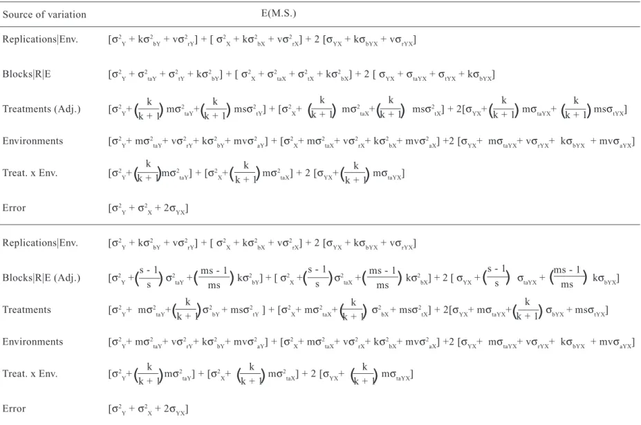
Table 3. Expected mean squares of the joint analyses of variance of square lattices, considering random model, in relation to the variable Y+X

Replications|Env. [σ2

Y + kσ2bY + vσ2rY] + [ σ2X + kσ2bX + vσ2rX] + 2 [σYX + kσbYX + vσrYX]

Blocks|R|E [σ2

Y + σ2taY + σ2tY + kσ2bY] + [ σ2X + σ2taX + σ2tX + kσ2bX] + 2 [ σYX + σtaYX + σtYX + kσbYX]

Treatments (Adj.) [σ2

Y+ mσ2taY+ msσ2tY] + [σ2X+ mσ2taX+ msσ2tX] + 2[σYX+ mσtaYX+ msσtYX]

Environments [σ2

Y+ mσ2taY+ vσ2rY+ kσ2bY+ mvσ2aY] + [σ2X+ mσ2taX+ vσ2rX+ kσ2bX+ mvσ2aX] +2 [σYX+ mσtaYX+ vσrYX+ kσbYX + mvσaYX]

Treat. x Env. [σ2

Y+ mσ2taY] + [σ2X+ mσ2taX] + 2 [σYX+ mσtaYX]

Error [σ2

Y + σ2X + 2σYX]

Blocks|R|E (Adj.) [σ2

Y + σ2taY + kσ2bY] + [ σ2X + σ2taX + kσ2bX] + 2 [ σYX + σtaYX + kσbYX]

Treatments [σ2

Y+ mσ2taY+ σ2bY + msσ2tY ] + [σ2X+ mσ2taX+ σ2bX + msσ2tX] + 2[σYX+ mσtaYX+ σbYX + msσtYX]

Environments [σ2

Y+ mσ2taY+ vσ2rY+ kσ2bY+ mvσ2aY] + [σ2X+ mσ2taX+ vσ2rX+ kσ2bX+ mvσ2aX] +2 [σYX+ mσtaYX+ vσrYX+ kσbYX + mvσaYX]

Treat. x Env. [σ2

Error [σ2

Y + σ2X + 2σYX]

k k + 1

)

(

k k + 1

)

(

kk + 1

)

k k + 1

(

)

(

k_{k + 1}

)

k k + 1

)

(

k k + 1

(

k_{k + 1}

)

(

ms - 1_ms

)

( )

s - 1_s

(

ms - 1_ms

)

(

s - 1_s

)

( )

s - 1_s

k k + 1

)

(

k_{k + 1}

)

(

k_{k + 1}

)

(

k_{k + 1}

)

k k + 1

(

)

(

k_{k + 1}

)

(

ms - 1_ms

)

k k + 1

(8)

The expected mean squares are identical to those presented for the random model, with

φa =

in the place of σ2

a. Therefore, the estimators of the

component σ2

t are identical to those of the random

model.

As seen, the statistical models (1), (2) and (3) are considered to estimate the covariance component due to treatment effect (σ_tYX), with a_gY, a_gX and a_g = a_gY + a_gX as fixed effects. Using previous results and since

the expected mean squares of the analyses of vari-ance of the variable Y + X are demonstrated. The ex-pected mean squares are identical to those presented for the random model, with φ_aY, φ_aX and φ_aYX in the place of σ2

aY, σ2aX and σaYX, respectively. Therefore,

the estimators of σ_tYX are equal to those of the ran-dom model.

2.2.2. Restricted mixed model

In the mixed model with the restriction

Σ

(ta)_ig = 0, to all i,

not all effects of interaction between treatment and environment are independent random variables.

In this model:

assuming that Cov[(ta)_ig , (ta)_ig’] = E[(ta)_ig(ta)_ig’] = σ, to all i, g and g’ (g • g’), we have:

σ = σ2 ta

Therefore, in the matrix Σ, C₀ = σ2

t + σ

2

r + σ

2

b + σ

2

ta + σ

2

C₁ = σ2

r + σ

2

b

C₂ = σ2

r

C₃ = σ2

t + σ

2

ta

C₄ = 0 C₅ = σ2

t σ

2

ta

C₆ = 0

Using the expectation of quadratic forms, the expected values below and those presented in Table 4 can be obtained:

E(Y’Y) = nµ2_{+ n}_σ2 t + nσ

2 r + nσ

2

b + mv

Σ

a 2

g + nσ 2

ta + n nσ2_{+ 2mvµ}

Σ

_a

g

E[R(µ)] = nµ + msσ2

t + vσ2r + kσ2b +

Σ

ag + σ2 + +2mvµ

Σ

a_g

E[R(µ, τ, δ, α, β)] = nµ2_{+ n}_σ2

Σ

a2g

+ mksσ2

ta + (v + mks - 1) σ2 + 2mvµ

Σ

ag

The estimators of σ2 t are:

1 s - 1

)

(

Σ a2

-g

g=1

s Σ g=1ag

)

s

(

2

=

₍

1_{s - 1}

₎

g=1Σ ag

s

Σ g=1

s

a_g- =

s

1 s - 1

)

(

s

= Σ_g=1s (a_g- a.)

2

1 s - 1

)

(

Σ (a_gY+ a_gX)

-g=1 s

)

Σ a_{gY +}a_gX)

g=1 s

(

2 = s

φ_a = 2

1 s - 1

)

(

Σ a2

-gY

g=1

s _g=1Σ agY

)

s

(

2

s

1 s - 1

)

(

Σ a2

-gX

g=1

s Σ _g=1agX

)

s

(

2

s +

1 s - 1

)

(

_Σ_(a

-gYagX )

g=1 s

(

+2 g=1Σ agY

)

s

(

s

)

Σ a_gX

g=1 s

(

2

=

= φ_aY+ φ_aX+ 2φ_aYX

1 s - 1

)

-V

Σ

(ta)_ig

g=1

s s

g=1

= sσ2

ta + 2

Σ Σ

Cov[(ta)ig, (ta)ig’] = 0,

[

]

g=1 s

(9)

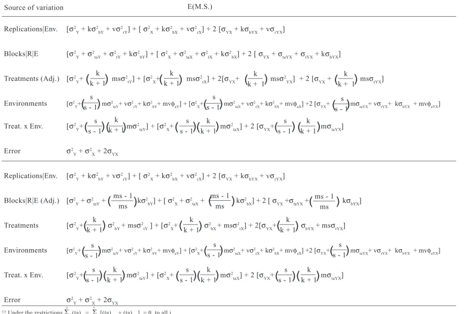
Table 4. Expected mean squares of the joint analyses of variance of square lattices, considering restricted mixed model1_{with environment effect fixed and other effects random}

Replications|Environment ... σ2_{+ k}σ2 b + vσ2b

Blocks|Rep.|Env. ... σ2 ₊ σ2

ta + σ2t + kσ2b

Treatments (Adjusted) ... σ2 _{+ ms}_σ2 t

Environments ... σ2 _{+ m}_σ2 ta+vσ

2 r+ kσ

2 b + mvφ

2 a

Treatments x Environments ... σ2 _{+ m}_σ2 ta

Error ... σ2

Replications|Environment ... σ2_{+ k}_σ2 b + vσ2r

Blocks|Rep.|Env. (Adjusted) ... σ2_{+ k}_σ2 b

Treatments ... σ2₊σ2

b + msσ2t

Environments ... σ2 _{+ m}_σ2

ta+vσ2r+ kσ2b + mvφa

Treatments x Environments ... σ2 _{+ m}σ2 ta

Error ... σ2

s - 1

)

(

k + 1 k

)

(

=

k k + 1

σ2

t(1)

[

]

MST(Adj.) - MSe ms

^_σ2 t(2) =

^

MST(N.Adj.) - MSe - σ2 b(2)

ms

≠

[

]

MST(N.Adj.) - MSe_CB ms

where: ^ ₌ ms

k(ms-1)

[

MSBRE(Adj.) - MSe -

₍

_s

₎

₍

k + 1

₎

₍

MST - MSe

₎

m

]

and MSe_CB is the error mean square, considering the com-plete block model. Therefore, σ2

t(2) is not the estimator of σ2

t of the analysis according to the complete block model.

The statistical models (1), (2) and (3) are ad-justed to estimate the covariance component σ_tYX.

Based on previous results and on the assumptions about the restricted mixed model, and since not all effects (ta)_ig = (ta)_igY + (ta)_igX are independent, the ex-pected mean squares presented in Table 5 are demon-strated. The estimators of σ_tYXare:

^

(1)_{Under the restrictions = 0, to all i.}

k

k + 1

s

s - 1

k

k + 1

k

k + 1

k

k + 1

ms - 1

ms

(

)

(

)

(

s

s - 1

)

(

s

s - 1

)

(

σ2 ta+

s

s - 1

)

(

Σ

(ta)_ig

s

g = 1 σ2

b(2)

^

(10)

3. APPLICATION

The results of the analyses of variance for height and diameter of 49 half-sib families of Euca-lyptus pyrocarpa, from a non inbred population, evalu-ated in a 7 x 7 simple lattice in two different environ-mental conditions, are shown in Table 6. The SAEG (System for Statistical Analyses) program, developed by the Universidade Federal de Viçosa, was used for the analyses.

Considering unrestricted mixed model, the analyses of variance show, at a level of 5% of signifi-cance, absence of interaction between families and environments, for height and diameter. There is no difference between the means of the reference popu-lation in the two environments (two levels of fertil-ization were used). In the base population there is genetic variability for both characters. As there is evidence of absence of progeny x environment inter-action, selection can be done considering the means

σtYX(1) =

where:

σYX =

σ_bYX(2) =

σ_taYX =

k k + 1

)

(

k + 1 k

)

(

{

[MST(Adj.)(Y + X) - MST(Adj.)(Y) - MST(Adj.)(X)] - [ MSe(Y + X) - MSe(Y) - MSe(X)]_2ms

}

^

MST(N.Adj.)(Y + X) - MST(N.Adj.)(Y) - MST(N.Adj.)(X) - 2σYX - 2 σbYX(2)

2ms

^ ^

σtYX(2) =

MSe(Y + X) - MSe(Y) - MSe(X) 2

^ ^

]

[

^ ms

2k(ms - 1) [MSB≠R≠E(Adj.)(Y + X) - MSB≠R≠E(Adj.)(Y) - MSB≠R≠E(Adj.)(X) - 2σYX - 2σtaYX] ^

k + 1 k

)

(

s - 1 s

)

(

^

₍

MSTE(Y + X) - MSTE(Y) - MSTE(X) - 2σtaYX

)

2m

of the families in the two levels of fertilization, fa-voring the choice of those with desired performance in different environments. Estimates of the genotypic variance between progenies, of the covariance between genotypic means of same family, and of some other genetic parameters are presented in Table 7. The equal-ity between the estimates of σ2

t(1)and σ2t(2) and of σt(1)

and σ_t(2) , reveals homogeneity between blocks within replication within environment.

In relation to both characters, the differences between the additive genetic values of the individuals in the base population account for a relevant portion of the variance of the phenotypic means of the fami-lies. The magnitude of the two heritabilities indi-cates that the families with greater phenotypic mean should have a common parent with greater additive genetic value (greater number of genes which increase each trait). The estimates of the correlation between the phenotypic mean of the family and the additive

^

(11)

ESTIMA

TION OF GENETIC P

ARAMETERS IN

THE

A

N

AL

YSIS OF SQ

U

ARE LA

TTICE...

20

5

Table 5. Expected mean squares of the joint analyses of variance of square lattices, considering restricted mixed model1_{with environment effect}

fixed and other effects random, in relation to the variable Y+X

Blocks|R|E [σ2

Y + σ2taY + σ2tY + kσ2bY] + [ σ2X + σ2taX + σ2tX + kσ2bX] + 2 [ σYX + σtaYX + σtYX + kσbYX]

Treatments (Adj.) [σ2

Y+ msσ2tY] + [σ2X+ msσ2tX] + 2[σYX+ msσ2YX] + 2 [σYX + msσtYX]

Environments [σ2

Y+ mσ2taY+ vσ2rY+ kσ2bY+ mvφaY] + [σ2X+ mσ2taX+ vσ2rX+ kσ2bX+ mvφaX] +2 [σYX+ mσtaYX+ vσrYX+ kσbYX + mvφaYX]

Treat. x Env. [σ2

Error σ2

Y + σ2X + 2σYX

Blocks|R|E (Adj.) [σ2

Y + σ2taY + kσ2bY] + [ σ2X + σ2taX + kσ2bX] + 2 [ σYX +σtaYX + kσbYX]

Treatments [σ2

Y+ σ2bY + msσ2tY ] + [σ2X+ σ2bX + msσ2tX] + 2[σYX+ σbYX + msσtYX]

Environments [σ2

Y+ mσ2taY+ vσ2rY+ kσ2bY+ mvφaY] + [σ2X+ mσ2taX+ vσ2rX+ kσ2bX+ mvφaX] +2 [σYX+ mσtaYX+ vσrYX+ kσbYX + mvφaYX]

Treat. x Env. [σ2

Error σ2

Y + σ2X + 2σYX

)

k k + 1

)

(

k k + 1

)

(

s s - 1

)

(

k k + 1

)

(

ms - 1_ms

)

(

ms - 1_ms

)

k k + 1

)

(

k_{k + 1}

)

(

ms - 1_ms

k k + 1

)

(

k k + 1

)

(

k_{k + 1}

)

k k + 1

)

(

k_{k + 1}

)

s s - 1

)

(

s s - 1

)

(

s s - 1

)

(

s s - 1

)

(

s_{s - 1}

)

(

s_{s - 1}

)

s s - 1

)

(

s_{s - 1}

)

(

s_{s - 1}

)

s s - 1

)

(

k_{k + 1}

)

(

s_{s - 1}

)

(

k_{k + 1}

)

(1)_{Under the restrictions}Σ_(ta)

ig = g = 1Σ [(ta)igY + (ta)igX] = 0, to all i. s

g = 1 s

k k + 1

)

(12)

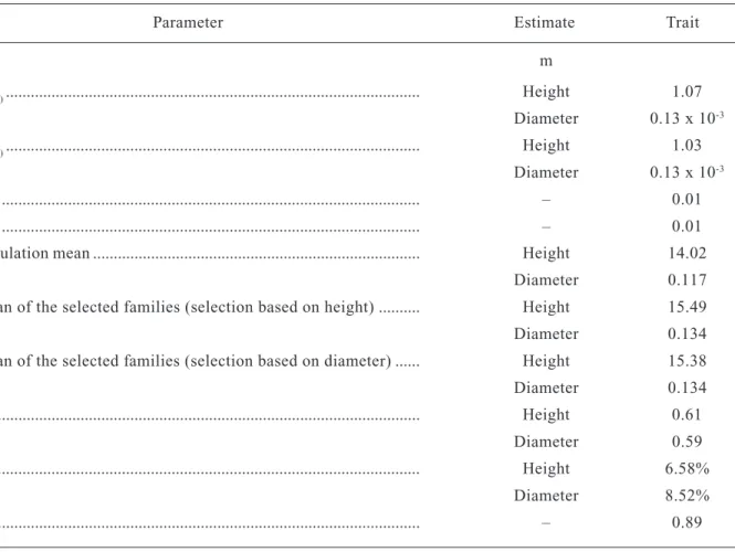
Table 7. Estimates of variance and covariance components and of some other genetic parameters1_{, in relation to}

height and diameter of half-sib families of a population of Eucalyptus pyrocarpa, evaluated in two environ-ments

σ2

t(1)... Height 1.07 ... Diameter 0.13 x 10-3 σ2

t(2)... Height 1.03 ... Diameter 0.13 x 10-3 σ_t(1)... – 0.01

σt(2)... – 0.01

Population mean ... Height 14.02

... Diameter 0.117 Mean of the selected families (selection based on height) ... Height 15.49

... Diameter 0.134 Mean of the selected families (selection based on diameter) ... Height 15.38

... Diameter 0.134 h2_... _Height _0.61

... Diameter 0.59

∆G... Height 6.58%

... Diameter 8.52% r_A... – 0.89

Parameter Estimate Trait

m

(1)_{The values of h}2_{(heritability in narrow sense, on a family mean basis),}_∆_{G (expected genetic gain due to selection and recombination}

of the 15 best families, expressed as percentage of the mean of the base population) and rA (additive genetic correlation between height

and diameter), were obtained considering the estimates of σ2

t(1) and σt(1) . The variance of the phenotypic means of the families was

estimated using the estimator MST(Adj.)/(k/(k + 1)) ms.

Table 6. Joint analyses of variance of height and diameter of 49 half-sib families of Eucalyptus pyrocarpa

Replications|Env. ... 2 6.7455 0.5862x10-3

Blocks|Rep.|Env. (Adj.) ... 24 1.9398 0.2496x10-3

Families (Adj.) ... 48 6.0997** _0.7704x10-3 **

Environments ... 1 13.0885ns _0.1046x10-2 ns

Families x Environments .... 48 2.3549ns _0.2987x10-3 ns

Error ... 72 1.7297 0.2148x10-3

Source of variation

Degrees of freedom

Mean square

Height Diameter

m m

(13)

genetic value of the common parent (Viana, 1996b) are š0.61 = 0.78 and š0.59 = 0.77, for height and diameter, respectively. Thus, the choice of the supe-rior families will alter the genotypic means of height and diameter of the base population, in the desirable direction. In relation to height, the predicted direct genetic gain with selection and recombination of the 15 best families (selection intensity of approximately 1.138) is of 6.58%. In relation to diameter, the ex-pected direct gain is 8.52%. The magnitude of the additive genetic correlation between the two traits (Viana, 1996a) shows that the direct selection based on one trait will determine indirect gain in relation to the other. The selection based on height should deter-mine a change in the mean diameter of the base popu-lation of (0.134 - 0.117) (0.59).100/0.117 = 8.57%. Evidently, there is no difference between the direct and indirect gains in relation to diameter (because of the equality between direct and indirect selection dif-ferentials). With selection considering diameter, the expected indirect gain for height is of (15.38 - 14.02) (0.61).100/14.02 = 5.92%.

REFERENCES

ARRIEL, E.F.; PACHECO, C.A.P. & RAMALHO, M.A.P. Evaluation of maize half-sib families in different plant densities. Pesquisa Agropecuária Brasileira, Brasília, 28(7):849-854, 1993.

BANCROFT, T.A. & SMITH, A.L. Efficiency of the simple lattice design relative to randomized complete blocks design in cotton variety and strain testing. Agronomy Journal, Madison, 41(4):157-160, 1949.

BENINATI, N.F. & BUSCH, R.H. Grain protein inheritance and nitrogen uptake and redistribution in a spring wheat cross. Crop Science, Madison, 32(6):1471-1475, 1992. CHAVES, L.J. & MIRANDA FILHO, J.B. de. Plot size for

progeny selection in maize (Zea mays L.). Theoretical and Applied Genetics, Berlin, 84(7/8):963-970, 1992. COCHRAN, W.G. & COX, G.M. Experimental designs. 2.ed.

New York, John Wiley & Sons, 1957. 611p.

FEDERER, W.T. Experimental design: theory and application.

New York, Macmillan, 1955. 544p.

FERRÃO, R.G.; GAMA, E.E.G. e; CARVALHO, H.W.L. de & FERRÃO, M.A.G. Evaluation of the combining ability of twenty maize lines in a partial diallel cross. Pesquisa Agropecuária Brasileira, Brasília, 29(12):1933-1939, 1994. GRAYBILL, F.A. Theory and application of the linear model.

North Scituate, Massachusetts, Duxbury Press, 1976. 704p.

JOHNSON, I.J. & MURPHY, H.C. Lattice and lattice square designs with oat uniformity data and in variety trials.

Journal of The American Society of Agronomy,

Washing-ton, 35(4):291-305, 1943.

KEMPTHORNE, O. An introduction to genetic statistics. New York, John Wiley & Sons, 1957. 545p.

LIN, C.S.; BINNS, M.R.; VOLDENG, H.D. & GUILLEMETTER, R. Performance of randomized block designs in field experiments. Agronomy Journal, Madison,

85(1):168-171, 1993.

MICHELINI, L.A. & HALLAUER, A.R. Evaluation of exotic and adapted maize (Zea mays L.) germplasm crosses.

Maydica, Bergamo, 38(4): 275-282, 1993.

MONCADA, P.; CASLER, M.D. & CLAYTON, M.K. An approach to reduce the time required for bean yield evaluation in coffee breeding. Crop Science, Madison,

33(3):448-452, 1993.

OLIVEIRA, A.C. de. Joint analysis of experiments in incomplete block designs with some common treatments - intrablock analysis. Pesquisa Agropecuaria Brasileira,

Brasília, 28(11):1255-1262, 1993.

REZENDE, G.D.S.P. & RAMALHO, M.A.P. Competitive ability of maize and common bean (Phaseolus vulgaris) cultivars intercropped in different environments. Journal of Agricultural Science, London, 123(2):185-190, 1994. SAHAGUN-CASTELLANOS, J. & FREY, K.J. Efficiency of

three experimental designs for genotype evaluation. Re-vista Chapingo, Chapingo, 15(71-72):114-122, 1990. SAS Institute, SAS/STAT®_._{User’s guide}_{. Version 6, 4.ed.}

Cary, NC, SAS Institute, 1989. v.1, 943 p.

SEARLE, S.R. Linear models. New York, John Wiley & Sons, 1971. 532p.

(14)

TORRIE, J.H.; SHANDS, H.L. & LEITH, B.D. Efficiency studies of types of design with small grain yield trials.

Journal of The American Society of Agronomy, Washing-ton, 35(8):645-661, 1943.

VIANA, J.M.S. Correlações entre médias genotípicas de mes-ma família. In: CONGRESSO NACIONAL DE MILHO E SORGO, 21., Londrina, 1996. Anais. Londrina,

Insti-tuto Agronômico do Paraná/Associação Brasileira de Mi-lho e Sorgo, 1996a. p.60.

VIANA, J.M.S. Herdabilidade em nível de média de família. In: CONGRESSO NACIONAL DE MILHO E SORGO, 21., Londrina, 1996. Anais. Londrina, Instituto Agronô-mico do Paraná/Associação Brasileira de Milho e Sorgo, 1996b. p.61.

WELLHAUSEN, E.J. The accuracy of incomplete block designs in varietal trials in West Virginia. Journal of the American Society of Agronomy, Washington, 35(1):66-76, 1943. ZUBER, M.S. Relative efficiency of incomplete block designs