ESTIMATION OF PHYSICAL AND CHEMICAL SOIL PROPERTIES BY
ARTIFICIAL NEURAL NETWORKS
1ROBERTO DIB BITTAR2*, SUELI MARTINS DE FREITAS ALVES2, FRANCISCO RAMOS DE MELO2
ABSTRACT - Soil physical and chemical analyses are relatively high-cost and time-consuming procedures. In the search for alternatives to predict these properties from a reduced number of soil samples, the use of Artificial Neural Networks (ANN) has been pointed out as a great computational technique to solve this problem by means of experience. This tool also has the ability to acquire knowledge and then apply it. This study aimed at using ANNs to estimate the physical and chemical properties of soil. The data came from the physical and chemical analysis of 120 sampling points, which were submitted to descriptive analysis, geostatistical analysis, and ANNs training and analysis. In the geostatistical analysis, the semivariogram model that best fitted the experimental variogram was verified for each soil property, and the ordinary kriging was used as an interpolation method. The ANNs were trained and selected based on their assertiveness in the mapping of considered standards, and then used to estimate all soil properties. The mean errors of ordinary kriging estimates were compared to those of ANNs and then compared to the original values using Student's t-Test. The results showed that the ANN had an assertiveness compatible with ordinary kriging. Therefore, such technique is a promising tool to estimate soil properties using a reduced number of soil samples.
Keywords: Artificial intelligence. Geostatistics. Precision agriculture. Soil management and conservation.
ESTIMATIVAS DE ATRIBUTOS DE FÍSICOS E QUÍMICOS DE SOLO POR MEIO DE REDES NEURAIS ARTIFICIAIS
RESUMO – O estudo das propriedades físicas e químicas do solo é um procedimento de custo e tempo relativamente elevado. Na busca de alternativas para predizer esses atributos a partir de um número menor de amostras do solo, o uso de Redes Neurais Artificiais (RNA) tem sido apontado como uma técnica computacional com grande capacidade de resolver problemas por meio da experiência, e possuem a capacidade de aquisição e posterior aplicação deste conhecimento. Esse trabalho teve por objetivo utilizar a RNA para estimar os atributos físicos e químicos de solo. Os dados utilizados foram provenientes da análise física e química de solo, coletados em 120 pontos amostrais, os quais foram submetidos à análise descritiva, análise geoestatística, treinamento e análise das RNAs. Na análise geoestatística, para cada atributo do solo, foi verificado o modelo de semivariograma que apresentou melhor ajuste ao modelo experimental, e como método de interpolação foi usada técnica da krigagem ordinária. As RNAs foram treinadas, selecionadas considerando a assertividade no mapeamento dos padrões considerados e utilizadas na estimativa de todos dos atributos de solo. O erro médio de cada estimativa obtida pela técnica da krigagem ordinária foi comparado com o erro médio da estimativa obtida pela RNA e, posteriormente foram comparadas com os valores originais por meio do teste-t de Student. Os resultados mostram que a técnica de RNAs apresenta assertividade compatível à krigagem ordinária. O uso da técnica de RNA apresentou-se promissora para obter estimativas de atributos de solo empregando um número menor de amostras de solo.
Palavras-chave: Inteligência artificial. Geoestatística. Agricultura de precisão. Manejo e conservação do solo.
____________________ *Corresponding author
1Received for publication in 02/19/2017; accepted in 09/20/2017. Paper extracted from the master dissertation of the first author.
2Agricultural Engineering Sector, Universidade Estadual de Goiás, Anápolis, GO, Brazil; [email protected] – ORCID: 0000-0002-5200
INTRODUCTION
Precision agriculture (PA) presents promising perspectives for crop management aimed at increasing productivity and optimizing production process, besides reducing environmental impacts from agricultural practices. A wide range of strategies can be used to minimize costs with agricultural inputs, such as tillage, planting, fertilizer use, and crop management (MOLIN; CASTRO, 2008; SOUZA et al., 2014). PA is a technological advance based on the principles of spatial variability and information management. Among the PA tools mostly used, georeferenced soil sampling has been traditionally used in Brazilian farming to characterize the variability of soil chemical properties (MONTANARI et al., 2012).
Knowing the spatial variability of soil properties allows us to describe a joint correlation of these variables, besides being fundamental for farming management (OLIVEIRA; FERNANDES; TEIXEIRA, 2011). The spatial continuity of a variable can be characterized by the similarity of its contents at two neighboring points in space. Such feature derives from a central tendency measure and/or a certain degree of spatial dependence in which close observations are associated, being greater in shorter distances. The level of spatial dependence significance is assessed by interpreting spatial dependence indexes (SEIDEL; OLIVEIRA, 2014). Soil properties are not distributed randomly within ecosystems; they follow a regionalized distribution. Some samples are more similar than others are, and such similarity varies with the distance between sampling points (SANTOS et al., 2013a). One of the limiting factors to represent this variation is regarding a number of samples needed to represent such distribution in the soil. The number of samples to be collected in the field to represent properly the distribution of soil properties is a frequent question among PA users. Since sampling is a costly and lengthy method, it often becomes unfeasible in practice (SOUZA et al., 2014).
In this aspect, geostatistical analysis has been widely used to determine the variability of soil properties in space. Notwithstanding, the number of sampled points and their distance are quite important to generate a reliable variogram in these analyses (YAMAMOTO; LANDIM, 2013; SOUZA et al., 2014).
Other technologies, such as Artificial Neural Networks (ANNs) are promising to estimate soil properties as well. ANNs are computational techniques inspired by the neural structure of intelligent organisms, acquiring knowledge through experiences and storing it. The ANNs comprise a flexible mathematical structure capable of performing non-linear mappings between input and output information. (NOROUZI et al., 2010; ANGELICO; SILVA, 2014). After some studies, Calderano Filho et al. (2014) confirmed the potential of using ANNs in the prediction of soil classes.
Based on the above, the objective of this study was to estimate physical and chemical properties of soil using Artificial Neural Networks (ANNs), as a technique of spatial variability determination.
MATERIAL AND METHODS
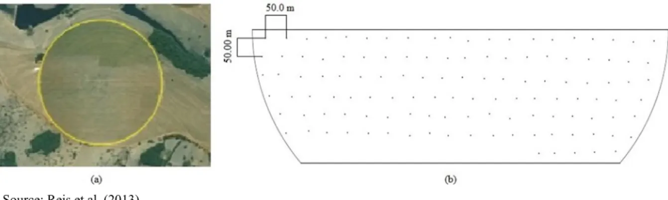
Field data were gathered from Palmital farm, in an area irrigated by central pivots within the city of Morrinhos – GO (Brazil). The location lies on an altitude of 813 m, latitude 17º45' S and longitude 49º10' W (Figure 1). Local soil type is classified as Dark-Red Latosol (Oxisol) with a sandy loam texture, according to the Brazilian Soil Classification System (SANTOS et al., 2013b).
All the collected data were georeferenced by means of a GPS recorder (Global Positioning System: ± 3m error), with real-time differential corrections via satellite and SAD69 datum system. These data were sampled from a 23-hectare area, in a sample grid of 120 points spaced in 50 x 50 m (Figure 1).
For each sampling point, five deformed soil samples were collected from the 0.0 to 0.20 m layer, within a one-meter radius around each sampling grid central point. The following soil properties were determined in these samples:
a) Chemicals: Hydrogen Potential (pH), Potassium (K), Phosphorus (P), Calcium (Ca), Magnesium (Mg), Exchangeable aluminum (Al3+),
Potential Acidity (H+Al), Organic Matter (OM) and Aluminum Saturation (m%);
b) Fertility: Cation Exchange Capacity (CEC) and Base Saturation (V%);
c) Physical: Clay, Sand, and Silt contents. All the 120 samples contained about 300 g soil were sent to a certified laboratory for soil chemical analyses, according to protocols described in Brazilian Manual of Soil Analysis methods (DONAGEMA et al., 2011).
From the original data, the descriptive measures for each variable (mean, median, mode, variance, standard deviation, and coefficient of variation) were estimated with the free R software.
The ANNs were trained using the MATLAB 2012 software (The Mathworks Inc.) with the application of the Neural Network Toolbox package, using a multilayer perceptron topology (MLP) feedforward with back-propagation error algorithm. The method used for the preparation, training, and application of ANNs was that proposed by Russel and Norvig (2013).
For each property (Table 1), 168 ANNs were trained. The network topology used in the training varied according to the number of: a) known soil samples (1, 2, 3 or 4); b) neurons in the hidden layer (3, 5, 7, 9, 13, 17 and 21), and c) training rounds (from 1 to 6). The input variables used for ANN training consisted of two parts:
Part 1: Estimated sampling point - soil sample with the values of each soil property to be estimated by the ANN. While training the ANN, this value is known and informed; yet, once the network is trained, this value will be the response revealed by the network to the geo-referenced location of a sampling point.
Part 2: Known sampling points - consisting of the already known soil samples. In the training, non-repetitive combinations of sampling points, different from the estimated sampling point, were used. The input variables increased according to the number of combined sampling points. The combination with one known sampling point generated 20 variables; the combination using two known sampling points generated 38 variables, and so on until the result of 74 variables for four known sampling points. We added 18 variables to each sampling point:
Geo-referenced location X of a known sampling point, which enabled calculating
the absolute distance to an estimated sampling point with geographic coordinate
X = DeltaXpoint;
Geo-referenced location Y of a known sampling point, which enabled calculating the absolute distance to an estimated sampling point with geographic coordinate Y = DeltaYpoint;
Altitude of the estimated sampling point, in meters;
Fifteen soil properties.
From the experimental data, four datasets were separated according to the following sequence:
Ten random sampling points used only in the final test of ANNs;
Training of 82 random sampling points;
Validation of 17 random sampling points;
Testing of 11 random sampling points. The number of samples of these sets was established by fitting the ratio indicated by Russel and Norvig (2013) due to the need to obtain integer values.
The ANN training process using MATLAB includes two data matrices. The matrix in which data is input is called input matrix, and that with the desired responses is called target matrix. For each studied property, four different input matrices and 15 target matrices were generated. While input matrices with one known sampling point contained 11,990 occurrences, those input matrices generated for 2, 3, or 4 points had 55,000 occurrences. A computational software developed for this purpose (BITTAR, 2016) generated all these matrices.
Both input and target matrix data were normalized to within a range from -1 to 1 (Equation 1), so the proportional magnitude of variables could be levelled for the ANN use.
(1) Where: y = normalization result;
x = value to be standardized;
xmin= X minimum value;
xmax= X maximum value;
d1 = normalization result lower limit;
d2 = normalization result upper limit.
Geographic coordinates and altitude of the sampling points were standardized using as a criterion for the lower limit, the minimum value found in the descriptive analysis subtracted by 10%; yet for the upper limit, the maximum value was increased by 10%. The soil properties were standardized using zero as the lower limit; yet for the upper limit, the maximum value defined by Alvarez et al. (1999) was chosen and; when not defined, the first prime number higher than the toxicity limit was then used.
The use of prime numbers as the upper limits aimed at avoiding standardizations equal to zero. Increasing the normalization range for training aims
to enable the ANN, after being trained, to be used in situations where the variables extrapolate the range of training values (HAYKIN, 2001).
An iterative software performed the ANN training, with an example generated by the MATLAB Neural Network toolbox. The next procedures were followed: loading of input and target data matrices; selection of parameters for the network training; designing of the ANN structure with the number of layers and neurons in each layer; updating of weights and bias-values; iterative
training until reaching the lowest overall error per dataset; ANN training interruption when the stopping criterion is reached. The
following values had to be observed concurrently: a) maximum number of learning cycles = 1,000; b) maximum number of failed cycles = 6; c) specialization or overfitting; d) minimum
performance gradient = 1 -15. Lastly, the trained network, its topology, bias, final weights, estimated values, compared values, and performance graphics are uploaded to a storage media.
From these uploaded training data, four ANNs were selected for each studied property, one for each known sampling point. These ANNs were chosen using, as a criterion, the lowest mean square error (MSE) from the input-output mapping. The MSE was calculated by comparing the output values with those of the target matrix (Equation 2). Haykin (2001) states that the lower the MSE value, the better the performance of an ANN.
(2) Where: n = number of elements;
Y = observed value; = estimated value.
The hit rate of each ANN was estimated by comparing network estimated and the observed values at the known sample points. For this, the MSE (Equation 2) and the mean relative error - P (Equation 3) were estimated considering two datasets: set C and set C2. While set C encompasses the values of the 120 known sampling points, C2 only comprises those of the final test dataset, which had not been mapped in the ANN training.
(3) Where: n = number of elements;
Y = experimentally observed value;
= estimated value.
The results estimated by the ANNs were denormalized (Equation 4) to perform this comparison.
MSE =1
n ( Yi-Yi)
2 n
i=1
𝑌
𝑃=100
𝑛
𝑌 − 𝑌 𝑌
𝑌
(4) Where: x = denormalization result,
y = normalized value;
xmin= X minimum value;
xmax= X maximum value;
d1 = normalization result lower limit;
d2 = normalization result upper limit.
The spatial dependence structure of the soil physical and chemical properties was identified by geostatistical analyses using the GS + version 10.0 software (Gamma Design Software). The model best fitting the experimental data was verified among the semivariograms models, for each studied soil property (ISAAKS; SRIVASTAVA, 1989). This model was selected based on the lowest residual sum of squares (RSS), the highest coefficient of determination (R²), and the highest cross-validation regression coefficient.
For the spatial dependence analysis, the spatial dependence index (SDI) was calculated as defined by Cambardella et al. (1994). Spatial dependence was considered weak when SDI was above or equal to 75%, moderate when between 25 and 75%, and strong if below or equal to 25% (Equation 5).
(5) Where: SDI = Spatial Dependence Index; Co = Nugget Effect;
(Co + C) = Sill.
For spatially dependent properties, ordinary kriging (OK) was used as an interpolation method, considering the calculated SDI. We have considered an isotropic spatial dependence, i.e. when spatial dependence is the same in all directions.
a.For each sampling point, the known values with spatial dependence were compared to those estimated by the selected ANNs and those estimated by OK. This procedure was done to contrast the assertiveness index of the selected ANNs with that of the OK. Finally, for each soil property, all the 120 sampling-point values were compared by P (Equation 6) in relation to:
a) Values estimated by ordinary kriging; b) Values estimated by ANN with 1, with 2, with 3, and with 4 known sampling points;
(6) Where: n = number of elements;
Y = experimentally observed value;
= estimated value.
Furthermore, the Student's t-test was employed to test whether there were any differences
𝑥= 𝑥𝑚𝑎𝑥 − 𝑥𝑚𝑖𝑛 ∗ 𝑦 − 𝑑1
(𝑑2− 𝑑1) +𝑥𝑚𝑖𝑛
𝑆𝐷𝐼= 𝐶0
(𝑐0+𝐶) 𝑥
100
𝑃=100
𝑛
𝑌 − 𝑌 𝑌
between the original values and those estimated by both OK and ANNs.
RESULTS AND DISCUSSION
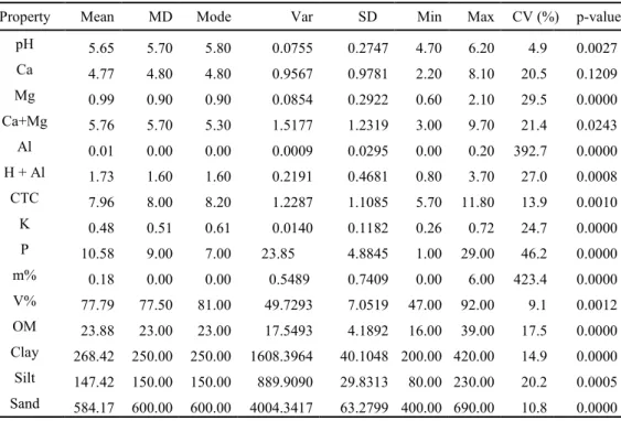
While the properties pH, K, V%, and sand content presented negative asymmetry, with mean and median lower than the mode, the other properties showed a positive asymmetry. Except for P, all the other properties showed no substantial variation for
mean, median, and mode values. This feature indicates that the sampled values might belong to a spatial distribution of varied values in regionalized distributions (Table 1).
The coefficients of variation (Table 1) for Al3+ and m% were above 200%, which is a high
value. Dias et al. (2015) also verified high CVs for Al3+, as well as mean and median values equal to
zero. On the other hand, pH, V%, and sand content presented low CVs, and the other properties showed medium values as classified by Warrick and Nielsen (1980) for field experiments.
Table 1. Descriptive analysis of soil physical and chemical properties.
Property Mean MD Mode Var SD Min Max CV (%) p-value
pH 5.65 5.70 5.80 0.0755 0.2747 4.70 6.20 4.9 0.0027
Ca 4.77 4.80 4.80 0.9567 0.9781 2.20 8.10 20.5 0.1209
Mg 0.99 0.90 0.90 0.0854 0.2922 0.60 2.10 29.5 0.0000
Ca+Mg 5.76 5.70 5.30 1.5177 1.2319 3.00 9.70 21.4 0.0243
Al 0.01 0.00 0.00 0.0009 0.0295 0.00 0.20 392.7 0.0000
H + Al 1.73 1.60 1.60 0.2191 0.4681 0.80 3.70 27.0 0.0008
CTC 7.96 8.00 8.20 1.2287 1.1085 5.70 11.80 13.9 0.0010
K 0.48 0.51 0.61 0.0140 0.1182 0.26 0.72 24.7 0.0000
P 10.58 9.00 7.00 23.85 4.8845 1.00 29.00 46.2 0.0000
m% 0.18 0.00 0.00 0.5489 0.7409 0.00 6.00 423.4 0.0000
V% 77.79 77.50 81.00 49.7293 7.0519 47.00 92.00 9.1 0.0012
OM 23.88 23.00 23.00 17.5493 4.1892 16.00 39.00 17.5 0.0000
Clay 268.42 250.00 250.00 1608.3964 40.1048 200.00 420.00 14.9 0.0000
Silt 147.42 150.00 150.00 889.9090 29.8313 80.00 230.00 20.2 0.0005
Sand 584.17 600.00 600.00 4004.3417 63.2799 400.00 690.00 10.8 0.0000
pH- Hydrogen potential; Ca – Calcium (cmolc dm-3); Mg - Magnesium (cmolc dm-3);
Al3+ – Exchangeable aluminum (cmolc dm-3); H+AL – Potential Acidity (cmolc dm-3); CEC - Cation
Exchange Capacity; P – Phosphorus (mg dm-3); K – Potassium (cmolc dm-3); m % - Aluminum saturation (%); V% - Base Saturation (%); OM- Organic Matter (g dm-3); Clay (g Kg-1); Silt (g Kg-1);
Sand (g Kg-1); MD – Median; Var - Variance; SD – Standard Deviation; Min – Minimum; Max – Maximum; CV(%)Coefficient of variation; p-value: Shapiro-Wilk’s test for normality at 5%
probability.
Likewise, Dias et al. (2015) found similar values for pH in the State of Goiás, when performing experiments in Latosols (Oxisols), with a mean of 5.46, a median of 5.50, and a CV of 3.72%. In the same research, these authors also observed CVs for K and V% that are similar to those observed here, but with distinct mean, median, maximum and minimum values.
The CEC mean value was 7.96 cmolc dm-³
(Table 1). According to Alvarez et al. (1999), soil fertility can be regarded as ‘average’ when considering the CEC. Based on the V% of 77.79% and respective CV below 9.07% found in this study (Table 1), we could consider the soil under study as
in good conditions for cropping (ALVAREZ et al., 1999).
From the geostatistical analysis, the semivariograms adjusted for the soil properties and the spatial dependence determination were
elaborated (Table 2). The properties pH, Ca, Ca + Mg, Al3+, H + Al, K, P, V%, Silt and Sand
Table 2. Theoretical models of semivariance adjusted to soil properties.
Property Semivariogram A0 C0 C0+C SDI RSS R2
pH PNE* - - - - - -
Ca PNE * - - - - - -
Mg Exponential 76.50 0.02 0.09 0.829 0.00014 0.46900
Ca+Mg PNE * - - - - - -
Al PNE * - - - -
H + Al PNE * - - - - - -
CTC Exponential 70.20 0.20 1.30 0.847 0.04930 0.23900
K PNE * - - - - - -
P PNE * - - - - - -
m% Exponential 204.90 0.31 0.61 0.501 0.08960 0.15400
V% PNE * - - - - - -
OM Spherical 69.30 0.09 17.11 0.995 6.14000 0.49400
Clay Exponential 57.30 177.00 1625.00 0.891 37175.00000 0.27400
Silt PNE * - - - - - -
Sand PNE * - - - - - -
A0- Range; C0 – Nugget Effect; C0+C - Sill, (SDI) Spatial Dependence Index; RSS – Residual sum of squares;
R2 - Regression coefficient, PNE* - Pure Nugget Effect; pH- Hydrogen Potential; Ca – Calcium; Mg - Magnesium; Al – Aluminum; H+AL – Potential Acidity; CEC - Cation exchange capacity;
P - Phosphorus; K – Potassium; m% - Aluminum saturation; V% - Base saturation; OM- Organic matter.
In spatial variability studies, the theoretical model must be adjusted since the linear estimator depends on the value of semivariogram model for each specified distance (SILVA NETO et al., 2016).
The exponential semivariogram model was best fitted for Mg, CEC, m%, and clay content; yet for OM, it was the spherical one (Table 2).
According to the classification proposed by Cambardella et al. (1994), Mg, CEC, OM, and clay content presented a weak spatial dependence for the area under study.
For the properties presenting spatial dependence, the OK technique was used, and then the values were compared with those estimated by the ANNs.
The ANN has as output matrix the estimates of all soil properties, regardless of spatial dependence. As described in the method of this study, the training matrix with one known sampling point was combined with all 109 other
samples. As for the training with 2, 3, and 4 samples, 550 combinations were drawn from the remaining
samples, to avoid repetition. The amount of data for the training with 2, 3, and 4 known samples was higher, but the number of possible combinations was not exhausted. The amount of training data was limited because the hardware and software could not
load the data matrix and its ANN training.
In the preliminary analysis of estimates from the selected ANNs (Table 3), m% reached the best hit rate with the selected ANN using four known sampling points, whereas CEC and V% achieved the best hit rate, with their respective selected ANNs, using three known sampling points. On the other side, the other properties presented better results with only one known sampling point, which might have been due to the number of combinations used for the training.
Five soil properties (pH, Al3+, m%, clay and
sand contents) were estimated by their respective selected ANNs presenting P (C) below 8% and P
(C2) below 9 % (Table 3). Six properties (Ca, Ca + Mg, CEC, V%, OM, and silt content) were
Table3. Results of selected ANN tests.
Property 1 soil sample 2 soil samples 3 soil samples 4 soil samples
P(C) P(C2) P(C) P(C2) P(C) P(C2) P(C) P(C2)
pH 3.13 5.62 5.30 7.63 5.62 7.82 5.34 7.88
Ca 14.15 18.49 17.37 22.12 19.00 22.96 17.73 22.74
Mg 16.25 20.58 26.56 25.47 24.63 25.73 25.60 26.67
Ca+Mg 14.69 18.53 17.63 21.54 19.22 22.38 18.69 22.33
Al 4.44 6.09 7.23 10.66 7.15 10.56 7.14 10.45
H+Al 15.65 21.48 31.22 37.93 29.95 36.58 29.19 35.50
CTC 9.89 13.89 10.91 14.87 9.94 13.73 10.51 14.07
K 17.78 23.91 29.48 40.42 28.43 39.03 28.44 40.00
P 30.26 41.49 48.54 69.19 45.89 65.43 46.03 66.20
m% 16.51 19.53 15.06 18.13 21.65 20.84 11.44 9.94
V% 15.80 12.10 15.86 13.88 12.71 9.85 15.49 12.78
OM 11.32 14.46 15.89 20.65 15.41 20.11 16.74 21.81
Clay 7.77 8.91 11.56 11.70 13.07 12.82 11.58 10.85
Silt 12.88 13.24 19.85 19.87 19.21 19.78 18.87 19.35
Sand 5.44 7.25 10.09 10.68 9.36 9.02 10.56 11.27
pH- Hydrogen potential; Ca – Calcium (cmolc dm-3); Mg - Magnesium; Al – Aluminum;
H+AL – Potential Acidity; CEC – Cation exchange capacity; P – Phosphorus; K – Potassium; m % - Aluminum saturation V% - Base saturation - OM- Organic Matter; P(C) – Relative mean error (%)
of set C consisting of 120 known sampling points; P(C2) – Relative mean error (%) of set C2 consisting of 10 known sampling points unmapped in the training of ANNs.
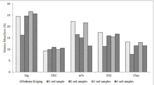
Regarding the spatial-dependent properties, CEC was best estimated by the OK method with a mean error of 9.29%, while ANN estimation using one known sampling point reached a mean error of 9.89%. The estimates of Mg, OM, m%, and clay presented better results using the respective artificial neural networks. The estimates of Mg, OM, and Clay had the lowest P using ANNs with one known
sampling point. Conversely, m% reached the best estimate result using ANN with four known sampling points (Figure 2). It is worth remembering that the 120 known soil samples were used to perform kriging, and for ANN, we used from 1 to 4 known sampling points, after training and selection (Figure 2).
The occurrence of any anomalous values within the studied area can directly affect estimate accuracy. Therefore, areas with uniform values generate most accurate estimates. On the other hand, if the values present a wider variance or outliers, estimate accuracy will be poor. Such an outcome is independent of the selected method, that is, any estimate will have better results in areas of low variability, and worse in those of high variability
(ISAAKS; SRIVASTAVA, 1989).
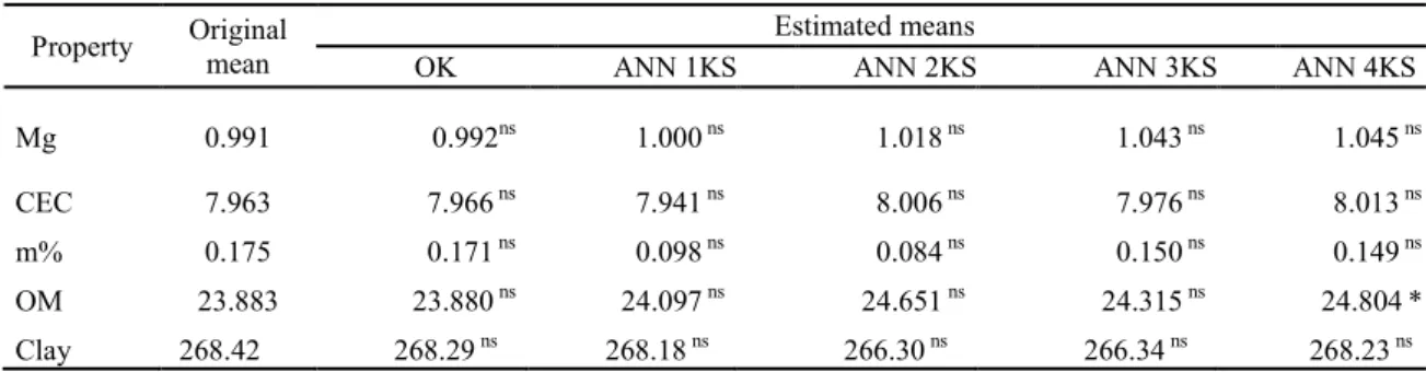
Both t-test results for spatial dependent properties among the 120 sample points, as well as the values estimated by OK and by the four ANNs selected, showed differences only for estimates of OM via ANN selected with four known sampling points, the other properties presented no differences (Table 4).
Table 4. Student's t-test for comparison between estimated and original data means, considering 120 sample points.
Property Original
mean
Estimated means
OK ANN 1KS ANN 2KS ANN 3KS ANN 4KS
Mg 0.991 0.992ns 1.000 ns 1.018 ns 1.043 ns 1.045 ns
CEC 7.963 7.966 ns 7.941 ns 8.006 ns 7.976 ns 8.013 ns
m% 0.175 0.171 ns 0.098 ns 0.084 ns 0.150 ns 0.149 ns
OM 23.883 23.880 ns 24.097 ns 24.651 ns 24.315 ns 24.804*
Clay 268.42 268.29 ns 268.18 ns 266.30 ns 266.34 ns 268.23 ns
Mg – Magnesium; CEC – Cation exchange capacity; OM- Organic Matter; m% - Aluminum Saturation;
OK - Ordinary Kriging; ANN 1KS - Artificial Neural Network with 1 Known Sampling point; ANN 2KS - Artificial
Neural Network with 2 Known Sampling points; ANN 3KS - Artificial Neural Network with 3 Known Sampling
points; ANN 4KS - Artificial Neural Network with 4 Known Sampling points. ns – non-significant at 5% probability
in relation to the original mean. * - significant at 5% probability in relation to the original mean.
CONCLUSIONS
The trained artificial neural networks acquired the necessary knowledge to estimate the results of the analyzed soil properties, regardless of its spatial dependence. The soil properties estimated by ANN, which in the geostatistical analysis presented spatial dependence, showed no significant differences in relation to the values estimated by ordinary kriging. The use of ANN has shown to be a promising technique to estimate soil physical and chemical properties from a reduced number of soil samples, which may represent a reduction in costs with laboratory analysis. Further studies are needed to improve the network and to increase the amount of data for training. The values of soil properties estimated by ANN are promising for spatial variability studies.
ACKNOWLEDGEMENTS
The authors thank the Foundation for Research Support of the State of Goiás (FAPEG) for granting the first author’s Masters Scholarship, and the State University of Goiás for the second author’s research incentive grant.
REFERENCES
ALVAREZ, V. H. et al. Interpretação dos resultados das análises de solo. In: RIBEIRO, A. C.; GUIMARÃES, P. T. G.; ALVAREZ, V. H. (Eds.). Recomendações para o uso de corretivos e fertilizantes em Minas Gerais - 5ª aproximação. Viçosa, MG: Comissão de Fertilidade do Solo do Estado de Minas Gerais, 1999. cap. 5, p. 25-32.
ANGELICO, J. C.; SILVA, I. N. Redes neurais artificiais aplicadas na estimativa da variabilidade de atributos do solo, SP. Revista Científica FACOL/ ISEOL, São Paulo, v. 1, n. 1, p. 9-20, 2014.
BITTAR, R. D. Redes neurais artificiais aplicadas à modelagem da variabilidade espacial de atributos físico-químicos de solos do cerrado. 2016. 112 f. Dissertação (Mestrado em Engenharia Agrícola: Área de Concentração em Engenharia de Sistemas Agroindustriais) - Universidade Estadual de Goiás, Anápolis, 2016.
CALDERANO FILHO, B. et al . Artificial neural networks applied for soil class prediction in mountainous landscape of the Serra do Mar. Revista Brasileira de Ciências do Solo, Viçosa, v. 38, n. 6, p. 1681-1693, 2014.
DIAS, M. J. et al. Probabilidade de ocorrência dos atributos químicos em um latossolo sob plantio direto. Revista Caatinga, Mossoró, v. 28, n. 4, p. 181-189, 2015.
DONAGEMA, G. K. et al. Manual de métodos de análise de solos. 2. ed. Rio de Janeiro, RJ: Embrapa Solos, 2011. 230 p.
HAYKIN, S. S. Redes neurais: princípios e práticas. 2. ed. Porto Alegre, RS: Bookman, 2001. 900 p. ISAAKS, E. H.; SRIVASTAVA, R. M. An introduction to applied geostatistics. New York: Oxford University Press, 1989. 561 p.
MONTANARI, R. et al. The use of scaled semivariograms to plan soil sampling in sugarcane fields. Precision Agriculture, Dordrecht, v. 13, n. 5, p. 542-552, 2012.
MOLIN J. P.; CASTRO C. N. Establishing management zones using soil electrical conductivity and other soil properties by the fuzzy clustering technique. Revista Scientia Agricola, Piracicaba, v. 65, n. 6, p. 567-573, 2008.
NOROUZI, M. et al. Predição da qualidade e quantidade do trigo de sequeiro utilizando rede neural artificial usando características de terreno e solo. Acta Agriculturae Scandinavica. Section B. Soil and Plant Science, Stockholm, v. 60, n. 4, p. 341-353. 2010.
OLIVEIRA, E. L. V.; FERNANDES, H. C.; TEIXEIRA, M. M. Variabilidade espacial das propriedades físicas de um latossolo amarelo eutrófico da região serrana do estado do Espírito Santo. Enciclopédia Biosfera, Goiânia. v. 7, n. 13, p. 1027-1042, 2011.
REIS, J. S. et al. Determinação de zonas de manejo para adubação nitrogenada em lavoura de tomate industrial. Revista Agrotecnologia, Anápolis, v. 4, n. 2, p. 68-84, 2013.
RUSSEL, S.; NORVIG, P. Inteligência artificial. 3. ed. Rio de Janeiro, RJ: Campus, 2013. 1016 p.
SANTOS, H. G. et al. Sistema Brasileiro de Classificação de Solos. 3. ed. Brasília, DF: Embrapa, 2013b. 353 p.
SANTOS, M. C. N. et al. Spatial Continuity of soil attributs in na Atlantic Forest remmant in the Mantiqueira Range, MG. Ciência Agrotecnologia, Lavras, v. 37, n. 1, p. 68-77, 2013a.
SEIDEL, E. J.; OLIVEIRA M. S. Proposta de um teste de hipótese para existência de dependência espacial em dados geoestatísticos. Boletim de Ciências Geodésicas, Curitiba, v. 20, n. 4, p. 750 -764, 2014.
SILVA NETO, S. P. et al. Variabilidade espacial da biomassa da forragem e taxa de lotação animal em pastagem de capim Marandu. Revista Agrogeoambiental, Pouso Alegre, v. 8, n. 2, p. 119 -130, 2016.
SOUZA, Z. M. et al. Número de amostras na análise geoestatística e na krigagem de mapas de atributos do solo. Ciência Rural, Santa Maria, v. 44, n. 2, p. 261-268, 2014.
YAMAMOTO, J. K.; LANDIM, P. M. B. Geoestatística: conceitos e aplicações. 1. ed. São Paulo, SP: Oficina de Textos, 2013. 215 p.