Determination of nitrogen and chlorophyll levels in bean-plant leaves
by using spectral vegetation bands and indices
1Discriminação de teores de nitrogênio e clorofila foliares do feijoeiro por meio de
bandas e índices de vegetação espectrais
Selma Alves Abrahão2*, Francisco de Assis de Carvalho Pinto3, Daniel Marçal de Queiroz2, Nerilson Terra
Santos4 e José Eustáquio de Souza Carneiro5
ABSTRACT -This study aimed to develop classifiers based on different combinations of spectral bands and vegetation indices from original, segmented and reflectance images in order to determine the levels of leaf nitrogen and chlorophyll in the bean, and to define the best time and best variables. A remote-sensing system was used, consisting of a helium balloon and two small-format digital cameras. Besides the individual spectral bands, four vegetation indices were tested: simple ratio, normalized difference, normalized difference in the green band, and modified-chlorophyll absorption. The classifiers proved to be efficient in determining levels of leaf nitrogen and chlorophyll. The best time for determining leaf N content was at 13 DAE (stage V4). The best classifiers for that time used as input variables two indices from segmented reflectance images, one index related to the canopy structure and the other related to chlorophyll, with a Kappa ranging from 0.26 to 0.31. The best time to discriminate leaf chlorophyll content was 21 DAE (stage V4). The best classifier used as input variables two original images, one in the red band and one in the blue with a Kappa of 0.47.
Key words:Precision farming. Remote sensing. Nitrogen dosage.
RESUMO - Objetivou-se desenvolver classificadores com base em diferentes combinações de bandas e índices de vegetação espectrais de imagens originais, segmentadas e reflectâncias, para discriminação de teores de nitrogênio e clorofila foliares do feijoeiro, definindo a melhor época e as melhores variáveis. Foi utilizado um sistema de sensoriamento remoto constituído por um balão a gás hélio e duas câmeras digitais de pequeno formato. Além das bandas isoladamente, foram testados quatro índices de vegetação: da razão simples, da diferença normalizada, da diferença normalizada utilizando a banda do verde e o da absorção de clorofila modificado. Os classificadores demonstraram serem eficientes na discriminação de teores de nitrogênio e clorofila foliares. A melhor época para discriminar teor de nitrogênio foliar foi aos 13 DAE (estádio V4). Os melhores classificadores para esta época utilizaram como entrada dois índices em imagens reflectância segmentada, um índice relacionado com a estrutura do dossel e outro relacionado com a clorofila, com Kappa variando entre 0,26 a 0,31. Para discriminar teor de clorofila foliar, a melhor época foi aos 21 DAE (estádio V4). O melhor classificador utilizou como entrada duas imagens originais, uma da banda vermelha e outra da banda azul, com Kappa de 0,47.
Palavras-chave: Agricultura de precisão. Sensoriamento remoto. Doses de nitrogênio.
* Autor para correspondência
1Recebido para publicação 29/11/2011; aprovado em 05/02/2013
Parte da Tese de Doutorado do primeiro autor apresentada ao Programa de Pós-Graduação em Engenharia Agrícola da Universidade Federal de Viçosa (UFV). Pesquisa financiada pela Fundação de Amparo à Pesquisa do Estado de Minas Gerais (FAPEMIG)
2Instituto Federal de Educação, Ciência e Tecnologia de Mato Grosso -Campus Cáceres, Avenida dos Ramires, s/n, Distrito Industrial, Cáceres-MT, Brasil, 78200-000, [email protected]
3Departamento de Engenharia Agrícola/UFV, Avenida P.H. Rolfs, s/n, Viçosa-MG, Brasil, 36.571-000, [email protected], [email protected] 4Departamento de Informática/UFV, Avenida P.H. Rolfs, s/n, Viçosa-MG, Brasil, 36.571-000, [email protected]
Rev. Ciênc. Agron., v. 44, n. 3, p. 464-473, jul-set, 2013 465
INTRODUCTION
The common bean is an agricultural product of economic and social importance as it occupies the fourth largest cultivated area in Brazil, along with soy, maize and cane sugar (IBGE, 2012), with its production process requiring a large contingent of labour during the crop cycle.
Despite the great potential, the average yield
of beans in Brazil, 951 kg ha-1 (IBGE, 2012), is
considered low. One major cause is due to the fact that this legume is still being cultivated mostly by small and medium producers who use a low technological level of production. Moreover, the bean is still grown in areas that require adjustment and fertilization, with conditions which limit the biological fixation of nitrogen, which is one of the limiting nutrients in bean
productivity (BRITOet al., 2009).
Precision agriculture is a developing technology that can be used as a tool in the advancement of agriculture, with remote sensing being one of the most promising of its techniques. The data obtained by remote sensing can be transformed into indices of vegetation, whose function is to maximize the variable under study, and minimise the various factors which cause variation, such as the architecture of the canopy, influence of the soil, stage of plant development,
geometry of the lighting and the sensor (GITELSONet
al., 1996; HABOUDANEet al., 2004).
Studies have been carried out on the development and evaluation of vegetation indices in order to determine their relation to the agronomic characteristics of the crops, such as analysis of crop growth, (BEZERRA; FIDELES FILHO, 2009), N
content of the leaves (ABRAHAMet al., 2009; CHEN
et al., 2010; EITELet al., 2008; LI et al., 2010) and
chlorophyll content of the leaves (EITELet al., 2009;
HABOUDANEet al., 2002; LIUet al., 2010; VINCINI;
FRAZZI, 2011).
In this study, the hypothesis was formulated that it is possible to discriminate classes of foliar nitrogen and chlorophyll levels in the bean using vegetation bands and indices, both alone and combined, obtained through remote sensing.
This work aimed to develop classifiers based on vegetation bands and indices, both alone and when combined, from original segmented and reflectance images, and use them to differentiate between levels of foliar nitrogen and chlorophyll in the bean, determining the best period and variables.
MATERIAL AND METHODS
The experiment was conducted at the Federal University of Viçosa, Florestal Campus in Minas Gerais, from March to July of 2010, on bean crops in the dry season. The bean variety BRSMG Majestic was cultivated, with type III growth pattern.
From the results of chemical analyses of the soil,
the addition of 5 t ha-1 lime (PRNT = 80% and MgO =
14%) to the soil was carried out on 12 February 2010.
At sowing, on 31 March 2010, 110 kg P2O5 ha-1 and
50 kg K2O ha-1 were applied manually, and uniformly
distributed, according to the recommendation of the
5th approximation (RIBEIROet al., 1999).
The soil was prepared by plowing once and harrowing twice. Sowing was carried out manually with a spacing of 0.5 m between rows and 12 seeds per metre at a depth of 0.05 m. Each plot consisted of five rows of 5.0 m, with an area of 12.5 m2. The ground area of each unit was made up of the three central rows, disregarding 0.5 m from each end of the lines, giving a total of 6.0 m2.
The treatments were comprised of a combination of nitrogen (N) both when the seeds were sown (0;
20 and 40 kg ha-1) and as top-dressing (0; 20; 40 and
60 kg ha-1), in a randomised-block design, with five
replications. The dosage of 20 kg N ha-1 was applied at 24 days after emergence (DAE) of the plants. Doses of 40 and 60 kg N ha-1 were divided equally at 19 and 29 DAE.
The bean plants were kept under irrigation with a conventional sprinkler. Other crop and plant-protection treatments were carried out following the needs of, and technical recommendations for, the bean plant in that region.
The remote sensing system, made up of an image acquisition system coupled to a helium balloon was used to acquire images of the bean canopy at three phenological stages of plant development: stage V4 (third trifoliate leaf) at 13; 21 and 26 DAE; stage R5 (pre-flowering) at 33 DAE; and stage R6 (flowering) at 41 DAE, under clear-sky conditions, and always at the same time, from 11:00 to 13:00 h.
The image acquisition system comprised two FUJIFILM FinePix model Z20fd digital cameras, positioned to point downwards, in order to acquire two simultaneous images of the same scene. For the remote control of the cameras, a system was developed of data communication via radio frequency, consisting of two electronic circuits, one for control of the camera and the other for shooting.
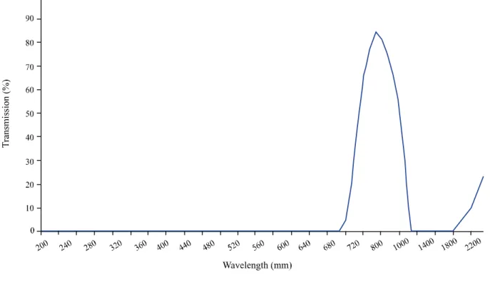
removed from one of the cameras and replaced by a Hoya RT-830 high-pass optical filter coupled to the camera lens, which allows radiation above 700 nm to pass (Figure 1).
In this way three images were acquired in the visible region (400 to 700 nm), i.e. bands of red (R), green (G) and blue (B), obtained with the color camera, and simultaneously an image in the near infrared region (NIR), obtained with the red sensor of the modified camera.
The images were saved in JPEG (Joint Photographic Experts Group) format, with dimensions of 3,648 by 2,736 pixels. The settings of the camera were: manual shooting mode; flash, anti-shake, intelligent face detection and red-eye removal all turned off; exposure compensation ± 0 EV, sensitivity ISO 64, white balance as in direct sunlight; center auto-focus mode.
As the cameras were set to acquire images focused at the centre, the plots that were in the upper and lower right and left corners were excluded due to being out of focus. Given the impossibility of placing the cameras at the same height in the field, due to the direction and altitude of the balloon being controlled by the buoyancy of the helium gas and the wind strength, a height of up to 30 m was used, this being the equivalent of a spatial resolution of 8 mm per pixel.
Figure 1 - Sensitivity of the Hoya RT-830 high-pass optical filter. Source: http://www.edmundoptics.com/techsupport/resource_center/
product_docs/curv_46444.pdf
To correct variations in the intensity of the pixels (digital levels) caused by changes in the ambient lighting, the images were calibrated with a radiometer. For calibration, we used a wooden panel, 12 x 1.8 cm, hand-painted in four levels of grey of 3 x 1.8 cm each, ordered from the highest to the lowest reflectance. The grey levels were obtained using a mixture of two acrylic fabric paints (Acrilex SPECIAL PAINT SA), one black (n.520) and the other white (n.519).
The panel was installed 0.15 m below the camera and inside its field of vision. This way, in all the images acquired, the panel appeared in the scene with a spatial resolution of approximately 0.04 mm per pixel. The digital levels from the image for each level of grey of the panel were obtained by calculating the average of the digital levels in a window of approximately 100 x 100 pixels, localized in the centre of the grey-level. The average values for reflectance of the grey levels of the panel were determined by means of a FieldSpec ® spectroradiometer, used to obtain data of between 325 and 1075 nm at a spectral resolution of 1 nm. Ten reflectance readings were taken for each gray level and the average value used for calibration.
Rev. Ciênc. Agron., v. 44, n. 3, p. 464-473, jul-set, 2013 467
by fitting a simple linear-regression equation to the levels extracted from the image for each window of the grey-level panel and the reflectance values (Equation 1):
(1)
where: = Reflectance in row i, column j, of band k, in %; = Regression constant; = Regression coefficient; and NC = Level of gray in row I, column j, of band k, non-dimensional. In each image acquired, windows were cut the size of the usable area of each plot. Four vegetation indices were determined (Equations 1; 2; 3; 4 and 5): RS=R/NIR (2)
NDVI=(NIR-R)/(NIR+R) (3)
MCARI1=1,2x[2,5x(NIR-R)-1,3x(NIR-G)] (4)
GNDVI=(NIR-G)/(NIR+G) (5)
where: RS = simple-ratio vegetation index (PEARSON; MILLAR, 1972); NDVI = normalized-difference vegetation index (ROUSE et al., 1974); MCARI1 = Modified chlorophyll-absorption index (HABOUDANE et al., 2004) ; GNDVI = normalized-difference vegetation index using the green band (GITELSONet al., 1996); G = Green band, R = Red band, and NIR = near-infrared band. The above-mentioned indices were also calculated using images segmented by the Otsu thresholding method (OTSU, 1974), with the aim of removing the effect of the ground on the images. The images obtained with the color camera, before undergoing thresholding, were processed with the normalized excess-green index EGD (MEYERet al., 1998): Egd=(2xG-R-B)/(G+R+B) (6)
where: B = Blue band. The levels of leaf-chlorophyll in each plot were determined using a SPAD 502 portable chlorophyll meter at the same times as the acquisition of the bean canopy images. For each plot, 30 SPAD values were randomly collected from leaves on the middle third of different plants. Values considered as outliers were not included in accordance with Equations 7 and 8 (BUSSAB; MORETTIN, 2002). The mean of the non-outlier values was considered as the SPAD value of the plot for each period. outliers>Q3+1,5(Q3-Q1) (7)
outliers<Q1+1,5(Q3-Q1) (8)
where: Q1 = first quartile (25%); and Q3 = Third
quartile (75%).
The same leaves used to determine the chlorophyll content, were collected as samples to determine the leaf N content in the laboratory by the Kjeldahl method. Two determinations were made, one at stage V4 at 13 DAE and the other at stage R6, at 41 DAE.
The values of N and leaf-chlorophyll were grouped into classes by visual analysis of the dendrograms. The dendrograms were obtained using the Ward method as the clustering algorithm, and Euclidean distance as the measure of dissimilarity (JOHNSON; WICHERN, 1998). To differentiate between the classes of N and leaf-chlorophyll, linear discriminant function statistical classifiers were developed (JOHNSON; WICHERN, 1998). For each period of image acquisition, 96 classifiers were tested (Table 1).
In order to obtain an unbiased estimate of classification errors, the technique of leave- one-out cross validation was used. The results of classification for the different feature vectors and periods were evaluated by developing the error matrix and calculating the Kappa
*In original, segmented-original, reflectance and segmented-reflectance images
Number of input variables (type of input variables) Number of classifiers
1 (R; G; B; NIR; NDVI; GNDVI; RS; MCARI1) 8 x 4* = 32
2 (R e G; R e B; G e B; NDVI e GNDVI; NDVI e RS; NDVI e MCARI1; GNDVI e RS;
GNDVI e MCARI1; RS e MCARI1) 9 x 4* = 36
3 (R, G e B; NDVI, GNDVI e RS; NDVI, GNDVI e MCARI1; GNDVI, RS e MCARI1;
NDVI, RS e MCARI1) 5 x 4* = 20
4 (R, G, B e NIR; NDVI, GNDVI, RS e MCARI1) 2 x 4* = 8
Total 96
coefficient (HUDSON; RAMM, 1987). The classifiers were evaluated by the Z-test of their Kappa coefficients at a level of significance of 5%.
To assist in the analysis of the classifiers, as proposed by Landis and Koch (1977), they were also classified into: Poor, when the value for the estimate of the Kappa coefficient is between 0.00 and 0.19; Reasonable, between 0.20 and 0.39; Good, between 0.40 and 0.59; Very good, between 0.60 and 0.79; and Excellent, when the Kappa value is greater than, or equal to 0.80.
Correlation analysis between leaf N content and SPAD values were also carried out.
RESULTS AND DISCUSSION
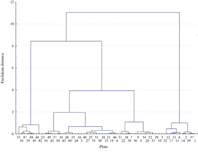
The dendrogram of the cluster analysis of leaf N content at stage V4 at 13 DAE is shown in Figure 2. The 60 plots were grouped into three classes of leaf N
Figure 2 - Dendrogram of the cluster analysis of leaf N content values at stage V4 at 13 DAE
content based on the point in the dendrogram where the Euclidean distance value gave the biggest jump.
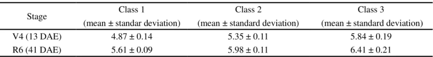
The values of leaf N observed at stage R6 at 41 DAE were grouped into three classes. This number of classes was defined based on the point in the dendrogram where the Euclidean distance value gave the biggest jump.
In general, the average values of leaf N for those classes obtained at stage R6 at 41 DAE tended to be higher than at stage V4 at 13 DAE (Table 2). This increase may be related to the effect of the nitrogen top-dressing, to the remains of previous crops, and also to the presence, as observed in the field, of nodules on the roots formed by bacteria of the genus Rhizobium, which obtain N by biological fixation. According to Ribeiro et al. (1999), the critical level of leaf N content, established
Rev. Ciênc. Agron., v. 44, n. 3, p. 464-473, jul-set, 2013 469
At stage V4 at 13 DAE, vegetation indices were calculated for 48 plots, as the images were not able to cover the entire experimental area. Of the 96 tested classifiers, three showed a Kappa coefficient statistically different from zero by the Z-test at 5% (Table 3).
The result of unsatisfactory ratings (reasonable ratings) is due to the stage of development of the bean. According to Britoet al. (2009), the increase in
N uptake is slow in the initial stages, and is therefore hardly stored or transported. This indicates that despite the experimental units having been exposed to different dosages of N, these differences had little effect on the N content observed in the leaves.
The result may also be related to the indices being better able to discriminate levels of leaf N where this is deficient, although not observed in the field (all plots showed leaf N content at stage V4 at 13 DAE above the critical level, between 3.0 and 3.5 kg dag-1). Similar results were found by Jensen et al. (2007) who used discriminant functions
based on visible and near-infrared bands for differentiating dosages of N in wheat. According to the authors, these data are best for differentiating N when deficient, in treatments of 0 and 40 kg ha-1, with 91% accuracy, instead of when there is an excess, in treatments of 80 kg ha-1 with 68% accuracy and 120 kg ha-1 with 58%.
We observed the importance of the combined effect of more than one vegetation index in the discrimination of the classes of leaf N content, since the three classifiers selected used as input a characteristic-vector with two indices, an index related to the canopy structure, indices that utilize the red and near infrared bands (RS and NDVI), and another related to the deficiency of chlorophyll, indices using the Green band (MCARI1 and GNDVI).
Table 2 - Average value and standard deviation for each class of leaf N content (dag kg-1) for each stage of bean development
Stage Class 1 Class 2 Class 3
(mean ± standar deviation) (mean ± standard deviation) (mean ± standard deviation)
V4 (13 DAE) 4.87 ± 0.14 5.35 ± 0.11 5.84 ± 0.19
R6 (41 DAE) 5.61 ± 0.09 5.98 ± 0.11 6.41 ± 0.21
** and *: significant at 1% and 5% respectively by the Z-test; Kappa coefficients followed by the same letter do not differ by Z-test at 5%
Table 3 - Classifiers selected for the discrimination of leaf N content based on the estimate of the Kappa coefficient at stage V4 at 13 DAE
Several authors have tested combinations of indices, albeit in the form of ratios, for example, MCARI/ OSAVI, TCARI/OSAVI and MCARI/MTVI2, and have reported that these combinations were more sensitive to changes in the levels of N and leaf chlorophyll content, than when using the indices individually, because these combined indices are able to minimize the effect of the leaf-area index and of the soil, and maximize the levels of N and leaf chlorophyll (EITELet al., 2008; EITELet al.,
2009; VINCINI; FRAZZI, 2011).
The three classifiers used segmented images. This result may be related to the stage of bean development. At the start of development, due to the low percentage of ground coverage by the plants, there was influence of ground reflectance, especially in the red band (digital level values higher than in the blue and green bands), and therefore in the vegetation indices that used this band. For this reason there was a tendency for the three classifiers to use segmented images, where the effect of the ground had been removed.
As the three classifiers were statistically identical by the Z-test at a significance level of 5%, and had the same number of input variables, the three were recommended for the classification of leaf N content for that period.
At stage R6 at 41 DAE, vegetation indices were calculated for 58 plots, as the images were not able to cover the entire experimental area. All the classifiers tested showed a Kappa coefficient statistically equal to zero by the Z-test at 5%, which means a performance equal to a random classification.
This late evaluation, in relation to the traditional period of cover fertilisation, was justified due to the
Image type Combinations Kappa Classification
Segmented-reflectance
MCARI1 e GNDVI 0.3119**a Reasonable
RS e MCARI1 0.2997**a Reasonable
results found by Britoet al. (2009). They determined that
N uptake occurs throughout the crop cycle, but that the period of higher demand, when N uptake is at a maximum, occurred between 58 and 68 days after seeding (DAS), at the start of pod maturation. However the results of that study do not corroborate Brito et al. (2009) where
vegetation indices were used to estimate leaf N content. This result indicates that in a more advanced stage, proper nutrition in all the plots resulted in the reflectance of the canopies matching, contrary to what happened at the beginning (stage V4 at 13 DAE).
Therefore, the best period to obtain images and discriminate between classes of leaf N content, was found to be at stage V4 at 13 DAE, before the period traditionally used to carry out top-dressing fertilization, at 25-30 DAE and before flowering takes place (RIBEIROet al., 1999).
The best classifiers for this period used as input two indices from segmented-reflectance images, one index related to the canopy structure (SR and NDVI) and the other related to chlorophyll deficiency (MCARI1 and GNDVI), with a Kappa ranging from 0.3119 to 0.2582.
There was a positive correlation (78.27%) between leaf N content and those SPAD values observed at stage V4 at 13 DAE, indicating that with the increase in N content there was an increase in the SPAD values.
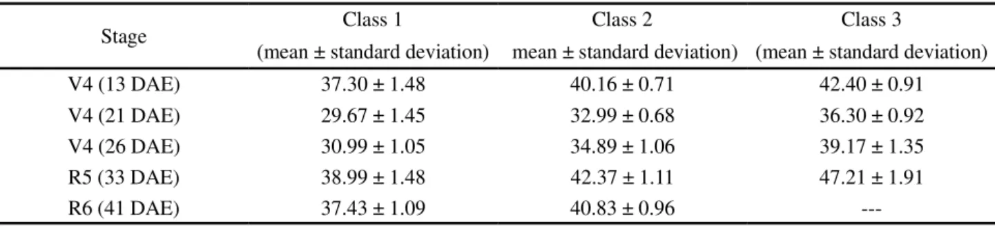
The 60 plots at stages V4 at 13; 21 and 26 DAE and R5 at 33 DAE, were grouped into three classes of SPAD value. At stage R6 at 41 DAE, they were grouped into two classes. The number of classes was defined based on the
Stage Class 1 Class 2 Class 3
(mean ± standard deviation) mean ± standard deviation) (mean ± standard deviation)
V4 (13 DAE) 37.30 ± 1.48 40.16 ± 0.71 42.40 ± 0.91
V4 (21 DAE) 29.67 ± 1.45 32.99 ± 0.68 36.30 ± 0.92
V4 (26 DAE) 30.99 ± 1.05 34.89 ± 1.06 39.17 ± 1.35
R5 (33 DAE) 38.99 ± 1.48 42.37 ± 1.11 47.21 ± 1.91
R6 (41 DAE) 37.43 ± 1.09 40.83 ± 0.96
---Table 4 - Mean value and standard deviation for each class of SPAD value and for each stage of bean development
point in the dendrogram where the Euclidean distance value gave the biggest jump. The mean value and standard deviation for the SPAD values for each class and stage were determined (Table 4).
At stage V4 at 13 DAE, vegetation indices were calculated for 48 plots, because the cameras were not able to cover the entire experimental area. Only one classifier, based on the four bands of the original images (R, G, B, NIR) showed a Kappa coefficient (Kappa = 0.2216) statistically different from zero by the Z-test at 5% with a classification of average.
This poor result (number of classifiers and reseanoble Kappa) may be related to the technology used being better able to discriminate levels of N and leaf chlorophyll where this is deficient, but this was not observed in the field. Similar results were found by Sant’Anaet al. (2010).
The result may also be related to the early development stage of the plant: despite the experimental units having been exposed to different dosages of N at seeding, these differences had little influence on the response of leaf chlorophyll content.
At stage V4 at 21 DAE, vegetation indices were calculated for 59 plots, as the cameras were unable to cover the entire experimental area. Of the 58 classifiers statistically different from zero by the Z-test at 5%, 54 classifiers were statistically equal or better at a 5% level of significance (Table 5).
Table 5 -Summary of classifiers selected for the discrimination of leaf chlorophyll content at stage V4 at 21 DAE
Image type Number of classifiers statistically different to zero % of Average % of Good
Original 19 89.47 10.53
Segmented-original 12 83.33 16.67
Reflectance 6 100.00 0.00
Rev. Ciênc. Agron., v. 44, n. 3, p. 464-473, jul-set, 2013 471
The 54 Kappa coefficients ranged from 0.2130 to 0.4724. Thus, the best classifiers were those obtained Kappa coefficients above 0.40, the simplest model and the least computational time. The best classifier being that which used a combination of two original images in the visible R and B (Kappa = 0.4724 **).
The SPAD 502 portable chlorophyll meter uses red electromagnetic radiation to determine the leaf chlorophyll content, and the near-infrared to compensate for differences in leaf thickness and water content
(ZOTARELLI et al., 2002). However, the absorption
peak of chlorophyll present in leaves is not only in the red band. Chlorophyll-a and -b are the pigments that most influence electromagnetic radiation in the visible region, with two absorption peaks, the larger in the red
band and the smaller in the blue respectively (LIMAet
al., 2011), favouring a better result for that classifier
using the red (R) and blue (B) bands.
At stage V4 at 26 DAE, vegetation indices were calculated for 54 plots, since the cameras were unable to cover the entire experimental area. Of the 96 classifiers tested, four showed a Kappa coefficient statistically different from zero by the Z-test at 5% probability (Table 6).
As the classifiers were statistically identical by the Z-test at a significance level of 5%, the best classifier for this period being the one using a combination of three
Table 6 - Classifiers selected for the discrimination of leaf chlorophyll content based on the estimate of the Kappa coefficient at stage V4 at 26 DAE
** and *: significant at 1% and 5% respectively by the Z-test; Kappa coefficients followed by the same letter do not differ by Z-test at 5%
Image type Combinations Kappa Classification
Original MCARI1, NDVI e RS 0.2453**a Reasonable
MCARI1, NDVI, GNDVI e RS 0.2038*a Reasonable
Reflectance G e B 0.2088*a Reasonable
R 0.2038*a Reasonable
indices, MCARI1, NDVI and RS from original images (Kappa = 0.2453 ** ) as they presented a simpler model (original images and a smaller number of indices) with less computational time. This model used a combination of three indices, two indices being related to the canopy structure (SR and NDVI) and one index related to chlorophyll deficiency (MCARI1).
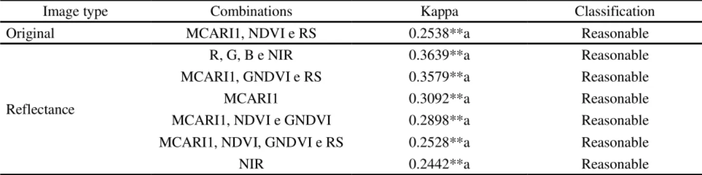
At stage R5 at 33 DAE, vegetation indices were calculated for 59 plots, since the cameras were not able to cover the entire experimental area. Of the 96 classifiers tested, seven showed a Kappa coefficient statistically different from zero by the Z-test at 5% probability (Table 7).
As the classifiers were statistically identical by the Z test at a significance level of 5%, the best classifier for this period was that using a combination of three indices, MCARI1, NDVI and RS (Kappa = 0.2538**) from original pictures. This classifier was also able to discriminate the leaf chlorophyll content as a function of the canopy structure (NDVI and SR) and of the chlorophyll deficiency (MCARI1).
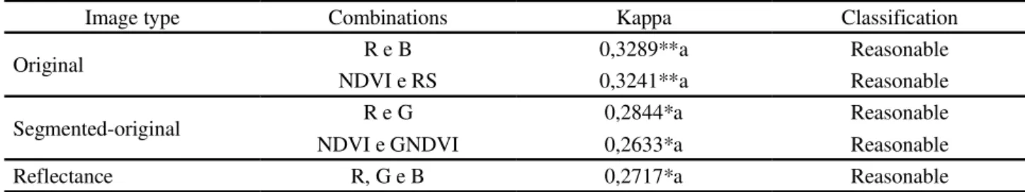
At stage R6 at 41 DAE, vegetation indices were calculated for 58 plots, as the cameras were not able to cover the entire experimental area. Of the 96 classifiers tested, five had Kappa coefficients statistically different from zero by the Z-test at 5% probability (Table 8).
Table 7 - Classifiers selected for the discrimination of leaf chlorophyll content based on the estimate of the Kappa coefficient at stage R5 at 33 DAE
Image type Combinations Kappa Classification
Original MCARI1, NDVI e RS 0.2538**a Reasonable
Reflectance
R, G, B e NIR 0.3639**a Reasonable
MCARI1, GNDVI e RS 0.3579**a Reasonable
MCARI1 0.3092**a Reasonable
MCARI1, NDVI e GNDVI 0.2898**a Reasonable
MCARI1, NDVI, GNDVI e RS 0.2528**a Reasonable
NIR 0.2442**a Reasonable
As the classifiers were statistically identical by the Z-test at a 5% level of significance, the best classifier for leaf chlorophyll content was that using a combination of two bands in the visible range, R and B (Kappa = 0.3289 **) from original images.
According to the results, the best time to determine the leaf chlorophyll content was at stage V4 at 21 DAE, before the period traditionally used to carry out cover fertilization at 25-30 DAE, (RIBEIROet al., 1999). This
result may be related to the leaf-area index; in this period the plots showed values for this index of less than two. When the leaf-area index reaches values of between two and three, increases in the leaf-area index do not influence the response of the crop in the visible region
(HABOUDANEet al., 2004).
To correct this limitation, several authors tested new vegetation indices and combinations of traditional vegetation indices, and reported that these new indices and combinations were more sensitive to variations in leaf N content and leaf chlorophyll content than when using the traditional individual indices (such as NDVI), since they are able to minimize the effect of the leaf-area index and of the ground, and maximize the leaf chlorophyll content (EITELet al., 2008; EITELet al.,
2009; VINCINI; FRAZZI, 2011).
Similar results were found in this study, depite not being the best periods to discriminate leaf chlorophyll content at 26 DAE (stage V4) and 33 DAE (stage R5), where all plots showed values for the leaf-area index of over two, there was a trend for the best results to come from those classifiers that used different combinations of indices.
CONCLUSIONS
1. The classifiers proved to be effective in discriminating classes of N content and leaf chlorophyll;
Table 8 -Classifiers selected for the discrimination of leaf chlorophyll content based on the estimate of the Kappa coefficient at stage R6 at 41 DAE
Image type Combinations Kappa Classification
Original R e B 0,3289**a Reasonable
NDVI e RS 0,3241**a Reasonable
Segmented-original R e G 0,2844*a Reasonable
NDVI e GNDVI 0,2633*a Reasonable
Reflectance R, G e B 0,2717*a Reasonable
**and *: significant at 1% and 5% respectively by the Z-test; Kappa coefficients followed by the same letter do not differ by Z-test at 5%
2. The best periode to discriminate classes of leaf N content was at stage V4 at 13 DAE. The best classifiers for this period used two indices from segmented-reflectance images as input, one index related to the canopy structure (SR and NDVI) and the other related to chlorophyll deficiency (MCARI1 and GNDVI), with a Kappa ranging from 0, 3119 to 0.2582;
3. To discriminate between classes of leaf chlorophyll content, the best period was at stage V4 at 21 DAE. The best classifier for this period used as input two original R and B images with a Kappa of 0.4724.
ACKNOWLEDGEMENTS
The authors wish to thank The National Council for Scientific and Technological Development (CNPq) and the Coordination for the Improvement of Higher Education Personnel (CAPES) for having granted their scholarship and The Foundation for the Support of Research of the State of Minas Gerais (FAPEMIG) for their financial support.
REFERENCES
ABRAHÃO, S. A.et al. Índices de vegetação de base espectral para discriminar doses de nitrogênio em capim-tanzânia.Revista Brasileira de Zootecnia, v. 38, n. 9, p. 1637-1644, 2009. BEZERRA, B. G.; FIDELES FILHO, J. Análise de crescimento da cultura do algodoeiro irrigada com águas residuárias.Revista Ciência Agronômica, v. 40, n. 3, p. 339-345, 2009.
BUSSAB, W. O.; MORETTIN, P. A.Estatística Básica. 5. ed. São Paulo: Saraiva, 2002. 540 p.
Rev. Ciênc. Agron., v. 44, n. 3, p. 464-473, jul-set, 2013 473 CHEN, P.et al. New spectral indicator assessing the ef ciency
of crop nitrogen treatment in corn and wheat.Remote Sensing of Environment, v. 114, n. 9, p. 1987-1997, 2010.
EITEL, J. U. H. et al. Combined spectral index to improve ground-based estimates of nitrogen status in dryland wheat.
Agronomy journal, v. 100, n. 6, p. 1694-1702, 2008.
EITEL, J. U. H. et al. Sensitivity of ground-based remote sensing estimates of wheat chlorophyll content to variation in soil re ectance.Soil Science Society of America Jounal, v. 73, n. 5, p. 1715-1723, 2009.
GITELSON, A. A.; KAUFMAN, Y. J.; MERZLYAK, M. N. Use of a green channel in remote sensing of global vegetation from EOS-MODIS.Remote Sensing of Environment, v. 58, n. 3, p. 289-298, 1996.
HABOUDANE, D. et al. Integration of hyperspectral vegetation indices for prediction of crop chlorophyll content for application to precision agriculture.Remote Sensing of Environment, v. 81, n. 2/3, p. 416-426, 2002.
HABOUDANE, D. et al. Hyperspectral vegetation indices and novel algorithms for predicting green LAI of crop canopies: Modeling and validation in the context of precision agriculture. Remote Sensing of Environment, v. 90, n. 3,
p. 337-352, 2004.
HUDSON, W. D.; RAMM, C. W. Correct formulation of the Kappa coefficient of agreement.Photogrammetric Engineering & Remote Sensing, v. 53, n. 4, p. 421-422, 1987.
INSTITUTO BRASILEIRO DE GEOGRAFIA E ESTATÍSTICA. Levantamento Sistemático da Produção Agrícola. 2012. Available: <http://www.ibge.gov.br/home/ estatistica/indicadores/agropecuaria/lspa/defaulttab.shtm.> Accessed: 20 abr. 2012.
JENSEN, T.et al. Detecting the attributes of a wheat crop using digital imagery acquired from a low-altitude platform.
Computers and Electronics in Agriculture, v. 59, n. 1/2, p. 66-77, 2007.
JOHNSON, R.A.; WICHERN, D.W. Applied multivariate statistical analysis. 4. ed. New Jersey: Prentice Hall, 1998. 816 p. LANDIS, J. R.; KOCH, G. G. The measurement of observer agreement for categorical data.Biometrics, v. 33, n. 1, p. 159-174, 1977.
LI, F. et al. Evaluating hyperspectral vegetation indices for estimating nitrogen concentration of winter wheat at different growth stages.Precision Agriculture, v. 11, n. 4, p. 335-357, 2010.
LIMA, N. et al. Sensoriamento remoto como ferramenta aos estudos de doenças de plantas agrícolas: uma revisão.Revista Brasileira de Geografia Física, v. 3, n. 2, p. 190-195, 2011.
LIU, M. et al. Neural-network model for estimating leaf chlorophyll concentration in rice under stress from heavy metals using four spectral indices.Biosystems Engineering,
v. 106, n. 3, p. 223-233, 2010.
MEYER, G. E.et al. Textural imaging and discriminant analysis for distinguishing weeds for spot spraying.Transactions of the ASAE, v. 41, n. 4, p.1189-1197, 1998.
OTSU, N. A threshold selection method from gray-level histograms.IEEE Transactions on Systems, v. 9, n. 1, p. 62-66, 1979.
PEARSON, R. L.; MILLER, R. D. Remote mapping of standing crop biomass for estimation of the productivity of the shortgrassprairie, Pawnee National Grasslands, Colorado. In: INTERNATIONAL SYMPOSIUM ON REMOTE SENSING OF ENVIROMENT, 8., Michigan.Proceedings... 1972, Michigan:
University of Michigan, 1972. p. 1355-1373. v. 2.
RIBEIRO, A. C.et al.Recomendações para o uso de corretivos e fertilizantes em Minas Gerais - 5a aproximação. Viçosa: UFV, 1999.
ROUSE, J. W. et al.Monitoring the vernal advancement of retrogradation (greenwave effect) of natural vegetation. Texas: College Station, 1974. 371 p.
SANT’ANA, E. V. P.; SANTOS, A. B.; SILVEIRA, P. M. Adubação nitrogenada na produtividade, leitura SPAD e teor de nitrogênio em folhas de feijoeiro. Pesquisa Agropecuária Tropical, v. 40, n. 4, p. 491-496, 2010.
VINCINI, M.; FRAZZI, E. Comparing narrow and broad-band vegetation indices to estimate leaf chlorophyll content in planophile crop canopies. Precision Agriculture, v. 12, n. 3, p. 334-344, 2011.