Inverse Problems in Science and Engineering Vol. 00, No. 00, January 2008, 1–17
RESEARCH ARTICLE
Localization of immersed obstacles from boundary measurements
Nuno F.M. Martinsa∗ and David Soaresb
aCEMAT-IST and Departamento de Matem´atica, Faculdade de Ciˆencias e Tecnologia,
Univ. Nova de Lisboa, Quinta da Torre, 2829-516 Caparica, Portugal;bDepartamento de
Matem´atica, Faculdade de Ciˆencias e Tecnologia, Univ. Nova de Lisboa, Quinta da Torre, 2829-516 Caparica, Portugal (Email:[email protected])
(v3.4 released May 2008)
A direct method for the localization of obstacles in a Stokes system is presented and the-oretically justified. The method is based on the so called reciprocity gap functional and is illustrated with several numerical simulations.
Keywords:Inverse obstacle problems; Stokes system; reciprocity functional; Stokeslets.
1. Introduction
In this work we consider the following inverse problem: a rigid body (obstacle)
occupies a region ω ⊂ R2 and is immersed in an incompressible viscous fluid,
occupying a bounded domain Ωc= Ω\ω. Inside this domain, Stokes system holds.
At the boundary, Dirichlet conditions are considered: a prescribed velocity at the
accessible part of the boundary, ∂Ω, and null velocity at the boundary of the
obstacle, ∂ω. On the other hand, the obstacle produces a stress tensor on ∂Ω
(measured data) from where we want to determine the location of the obstacle. This inverse problem is an example of an inverse obstacle problem in non destructive testing. Such problems have many applications in several engineering areas (see, for instance some examples in the book [1]). For the problem here considered we refer the work [2], where theoretical results concerning obstacle identification from boundary measurements and local stability were established. In [3] an iterative method based on the topological derivative and the Kohn-Vogelius functional is proposed for the identification of multiple 3D small obstacles and their location. In [4], a numerical shape reconstruction method based on integral equations was presented and tested. In this case, the location of the obstacle was assumed to be known. In [5], an optimization method for the reconstruction of both obstacle shape and location was proposed and tested (see also the work [6]). In this case, both shape and location were retrieved simultaneously with an iterative method.
Here, we propose a direct method for the location of a single 2D obstacle, based on Green’s formula for the Stokes equations. The method requires the computation of the so called reciprocity functional at appropriate test functions (see [7] for an application to the determination of point forces in a Stokes system) and can be easily adapted for the 3D case. This type of approach was presented in [8] for the
∗Corresponding author. Email: [email protected] ISSN: 1741-5977 print/ISSN 1741-5985 online
c
⃝2008 Taylor & Francis
reconstruction of cavities or inclusions in a Laplace problem (see also [9] for the localization of several circular obstacles using the reciprocity gap functional in a transmission problem for the Laplace equation). This work was partially presented by the authors at a conference on the Portuguese Naval School (cf. [10]) and is organized as follows: In section two, we define the inverse problem here addressed and the associated direct problem. In section three, we present some theoretical results concerning the identification of obstacles from a pair of Cauchy boundary data. Section four addresses the retrieving of the location using the reciprocity gap functional. We show that the proposed formulae for the location of the obstacle are related to the center of mass coordinates, for some density functions. Moreover, we show that, for some prescribed boundary velocities, the retrieved center of mass is related to the center of the whole domain, Ω. We conclude the paper with a section containing several numerical simulations to illustrate the proposed method.
2. Direct and inverse problems
Let Ω ⊂ R2 be a simply connected, open and bounded domain with regular C1
boundary Γ := ∂Ω, which we shall call a regular domain. Let ω be a regular
domain such that ω⊂⊂Ω, meaning that ω⊂Ω. Denote byγ the boundary of ω.
Define the domain of propagation Ωc := Ω\ω and notice that ∂Ωc = Γ∪γ. The
domain Ωc will represent the region occupied by the fluid whereasω is the region
occupied by the obstacle.
Given a boundary velocityg = (g1, g2) of the fluid at Γ, and the no-slip boundary
condition atγ, the system of equations governing the fluid flow here considered is
given by
µ∆u− ∇p=0 in Ωc
∇.u= 0 in Ωc
u=g on Γ =∂Ω
u=0 on γ =∂ω
, (1)
where u = (u1, u2) is the fluid velocity, p the pressure and µ the dynamic
vis-cosity, which we shall assume to be µ = 1. Recall that ∆u = (∆u1,∆u2) is the
Laplacian and∇pthe gradient of the pressure. The condition∇ ·u= 0 means that
uis solenoidal and represents the incompressibility of the fluid. This condition
im-plies that the prescribed boundary velocitygmust satisfy the no flux compatibility
condition
∫
Γ
g·ndσ= 0, (2)
wherenis the normal field at Γ, pointing outwards with respect to Ωc. The stress
tensor associated to the flux (u, p) is
T(u, p) :=−pI+ 2ϵ(u)
ϵ(u) = 1 2
(
∇u+∇u⊤)
is the stress strain tensor ofu. In particular, problem (1) can be written as
∇ ·T(u, p) =0 in Ωc
∇.u= 0 in Ωc
u=g on Γ =∂Ω
u=0 onγ =∂ω .
The direct problem consists in, given a boundary velocity g at Γ (satisfying the no flux condition (2)), determine the generated traction at Γ,
gn :=T(u, p)n|Γ (3)
where (u, p) satisfies Stokes system (1). It is well known that, takingg ∈H1σ/2(Γ),
where
H1σ/2(Γ) := {
g ∈(H1/2(Γ))2 : ∫
Γ
g·ndσ= 0 }
,
problem (1) is well posed, with (u, p)∈H1div(Ωc)×L2(Ωc)/R. The spaceH1div(Ωc)
is defined as the subspace of (H1(Ωc))2 such that∇ ·u= 0 in Ωc. Recall also that
the pressurepis unique up to an additive constant and that
L2(Ωc)/R∼=L20(Ωc), where
L20(Ωc) := {
p∈L2(Ωc) : ∫
Ωc
p= 0 }
.
In this functional setting we havegn∈H−1/2(Γ) =
(
H1/2(Γ))′.
The inverse problem consists in: given a pair of Cauchy data (g,gn)|Γ, where
gn is defined by (3), determine the location ofω. Here, we are assuming only the
knowledge of the exterior boundary Γ and that at the boundary of the obstacle,γ,
we have a no slip boundary condition (the geometry ofγ is, therefore, unknown).
3. Identification and reconstruction results
The following is a well known identification result of obstacles from a single pair of Cauchy boundary data.
Proposition 3.1 : ([2, 4]) Letω1, ω2 ⊂⊂Ωbe regular domains,g∈H1σ/2(Γ)\{0}
then
ω1 =ω2.
Using analytic continuation arguments, the previous identification result is also valid for Cauchy data in an open part of the boundary Γ.
3.1. Reconstruction of circular shaped obstacles
As a consequence of the above result, let us see the following particular case of localization of circular shaped obstacles. Let
Br(x0, y0) :={(x, y)∈R2 :||(x, y)−(x0, y0)||< r}
and suppose, by simplicity, that Ω =BR(0,0). Define the set of admissible circular
shaped obstacles
Ac ={Br(x0, y0) :Br(x0, y0)⊂⊂Ω}.
Givenω=Br(x0, y0)∈ Ac consider the vector field
u(x, y) = (
r2
(x−x0)2+ (y−y0)2 −1
)
(y−y0, x0−x)∈H1div(Ω\ω). (4)
It can be easily seen that the pair (u,0) satisfies Stokes system in the domain of
propagation Ωc = Ω\ω, considering the boundary velocity
g =u|Γ. (5)
On the other hand,
gn =T(u,0)n|Γ=
2r2
R((x−x0)2+ (y−y0)2)2
(
R2v1+v2) (6)
where
v1 = (y0−y, x−x0) and v2=(x20y−y0(2xx0+yy0),−y20x+x0(xx0+ 2yy0)).
Thus, we can define the map
Λ :Ac ∋Br(x0, y0)7→(g,gn)
with (g,gn)∈Hσ1/2(Γ)×H−1/2(Γ) defined by (5) and (6), respectively. By
Propo-sition 3.1, Λ is injective and, in particular, we have the following result.
Lemma 3.2 : Let (x0, y0, r) be such that Br(x0, y0)∈ Ac. Then,
(x0, y0, r) = argmin (x∗
0,y
∗
0,r∗)
s.t.Br∗(x∗0,y∗0)∈Ac
||g∗n−π2◦Λ(Br∗(x∗
where gn∗ is the traction at Γ generated by the obstacle Br(x0, y0) and considering
the boundary velocity g∗ =π
1◦Λ(Br∗(x∗ 0, y∗0)).
Proof : The mapπ1(respectivelyπ2) denotes the projection ofHσ1/2(Γ)×H−1/2(Γ)
ontoH1σ/2(Γ) (respectivelyH−1/2(Γ)). Notice that
π2◦Λ(Br(x0, y0)) =g∗n
whereg∗n is the traction at Γ generated by Br(x0, y0) and considering the velocity
g∗ =π1◦Λ(Br(x0, y0)). In particular,
||g∗n−π2◦Λ(Br(x0, y0))||= 0
and the triplet (x0, y0, r) is a solution of the above minimization problem. We now
prove that it is unique. Let (x∗
0, y0∗, r∗) be such that ||gn∗ −π2◦Λ(Br∗(x∗
0, y∗0))||= 0.
Then,
Λ(Br∗(x∗
0, y∗0))) = (g∗,gn∗) = Λ(Br(x0, y0))
and the result follows from the injectivity of Λ.
This lemma shows that the reconstruction of circular shaped obstacles can be obtained by solving the above minimization problem. However, it requires several boundary measurements which is a drawback, when comparing with the iterative method proposed in [5]. Moreover, it relies on an explicit solution of Stokes system for circular shaped obstacles and it cannot be generalized for other type of obstacles.
4. Recovering the location of an obstacle using the reciprocity functional
Here we propose a method based on Green’s formula for the location of the obstacle. It requires only one boundary measurement and does not depend on the shape of the obstacle.
Given a regular domain ω⊂R2 and a regular functionf :ω→R with constant
sign, the mass center ofω with densityf is the pair (xf, yf) defined by
xf = ∫
ω
xf(x, y)dA
∫
ω
f(x, y)dA
and yf =
∫
ω
yf(x, y)dA
∫
ω
f(x, y)dA .
In particular, when the density is constant, we obtain the so called center of
gravity (x, y)
x= ∫
ω
xdA
|ω| and y=
∫
ω
ydA
where |ω| is the area of ω. Suppose that ω has C2 boundary. Since for a density
functionf ∈L2(ω) there exists an unique u∈H2(ω) satisfying
{
∆u=f inω
u= 0 onγ =∂ω
then, second Green’s formula (eg. [11]) yields, for a test functionv∈H2(ω),
∫
ω
(∆uv−u∆v)dA=
∫
γ
(∂nuv−u∂nv)dσ,
where ∂nu := ∇u·n|γ is the normal derivative at γ. In particular, taking the
harmonic test functionv(x, y) =xwe have
∫
ω
f(x, y)xdA= ∫
γ
∂nuxdσ.
Therefore, we can also write the center of mass (xf, yf) using only boundary
integrals,
xf = ∫
γ
∂nuxdσ
∫
γ
∂nudσ
and yf =
∫
γ
∂nuydσ
∫
γ
∂nudσ
. (8)
In particular, for the center of gravity, that is assuming f ≡1, we get
x= ∫
γ
∂nu1xdσ
∫
γ
∂nu1dσ
and y=
∫
γ
∂nu1ydσ
∫
γ
∂nu1dσ
(9)
where u1 is given by
u1=uh+
x2
2 ,
and uh is the harmonic function in ω such that
uh|γ =−x
2
2 |γ.
4.1. Center of a circle
For the particular case of circular domains ω = Br(x0, y0), it is well known that
u(x0, y0) = ∫ γ udσ ∫ γ dσ , (10)
for any harmonic function u in ω. Thus, considering the harmonic functions
u1(x, y) = x and u2(x, y) = y we have, by (10), the following identity for the
geometric center ofω,
x0 =
∫ γ xdσ ∫ γ dσ
and y0 =
∫ γ ydσ ∫ γ dσ .
Notice that this formula coincides with (7). In fact, for f(x, y)≡1, the function
u(x, y) = 1
4(x−x0)
2+1
4(y−y0)
2−r2
4
satisfies
∆u=f inω =Br(x0, y0)
u= 0 on γ =∂Br(x0, y0) ∂nu= r2 on γ
. Hence, x= ∫ ω xdA ∫ ω dA = ∫ ω
f(x, y)xdA
∫
ω
f(x, y)dA
= ∫
γ
∂nuxdσ
∫
γ
∂nudσ
= ∫ γ xdσ ∫ γ dσ
=x0.
4.2. Reciprocity functional for Stokes equations
Let (u, p) and (v, q)∈(H2(Ωc)∩Hdiv1 (Ωc))×H1(Ωc), where Ωc = Ω\ω andω,Ω
are any C2 regular domains. Assuming that the normal at ∂Ωc = Γ∪γ points
outwards with respect to Ωc, we have the following Gauss-Green formula
∫
Ωc
((∆u− ∇p)·v−u·(∆v− ∇q))dA=
∫
Γ
(T(u, p)n·v−u·T(v, q)n)dσ
+ ∫
γ
(T(u, p)n·v−u·T(v, q)n)dσ.
Given (u, p), we define the reciprocity functional at Γ
RΓ(v, q) :=
∫
Γ
In the following, we shall assume that (u, p) satisfies Stokes system (1). Hence,
RΓ(v, q) =
∫
Γ
(gn·v−g·T(v, q)n)dσ (12)
where (g,gn) is the pair of Cauchy data at Γ (recall that this data is assumed to
be available in the inverse problem). Gauss-Green formula gives
RΓ(v, q) =−
∫
Ωc
u·(∆v− ∇q)dA−
∫
γ
T(u, p)n·vdσ. (13)
4.3. Formulae for the center of mass
Suppose that the pair of test functions (v, q) satisfy
∆v− ∇q = 0 in Ωc.
Then, using (13) we can write the identity
RΓ(v, q) =−
∫
γ
T(u, p)n·vdσ
from where we can obtain the following reconstruction method for the center of mass.
Take q≡0 and
v1(x, y) =x⃗e2 ∈H2(Ω)∩H1div(Ω) (14)
where (⃗e1, ⃗e2) is the standard basis inR2. We have,
RΓ(v1,0) =−
∫
γ
T(u, p)n·⃗e2xdσ.
On the other hand,
RΓ(⃗e2,0) =−
∫
γ
T(u, p)n·⃗e2dσ
hence, assuming RΓ(⃗e2,0)̸= 0 we get the approximation
RΓ(v1,0) RΓ(⃗e2,0)
(15)
for the first coordinate. For the second coordinate, we consider
and obtain
RΓ(v2,0) RΓ(⃗e1,0)
. (17)
Remark 1 : The above formulae (15) and (17) require only a single pair of Cauchy
data (g,gn) on Γ. On the other hand, no information regarding the shape of ω is
considered.
The following result shows that in certain cases, the formulae (15) and (17) provides the coordinates of the obstacle, for some density functions.
Proposition 4.1 : Suppose thatT(u, p)n|γ∈H1/2(γ). There existsf1, f2 ∈L2(ω)
such that
RΓ(v1,0) RΓ(⃗e2,0)
=xf1 and
RΓ(v2,0) RΓ(⃗e1,0)
=yf2.
Moreover,
xf1 =
RΓ
(
−∫ 1
ωxdA
v1,0
)
RΓ(−|ω|−1⃗e2,0)
x and yf2 =
RΓ
(
−∫ 1
ωydA
v2,0
)
RΓ(−|ω|−1⃗e1,0)
y (18)
where (x, y) is the center of gravity of ω.
Proof : We show the above identities for the first coordinate (the second can be
obtained in the same manner). Leteg=−T(u, p)n·⃗e2 ∈H1/2(γ). Since the bilaplace
problem
∆2w= 0 inω
w= 0 on γ ∂nw=eg on γ
is well posed inH2(ω) (eg. [11]) then, for f
1= ∆w∈L2(ω) Green’s formula yields
∫
ω
f1vdA=
∫
ω
(∆wv−w∆v)dA=
∫
γ
(∂nwv−w∂nv)dσ=
∫
γe
gvdσ,
for every harmonic test functionv. Therefore, takingv=x we get
∫
ω
f1xdA=RΓ(v1,0).
Since we also have∫ωf1dA=RΓ(⃗e2,0) then,
xf1 = ∫
ωf1xdA
∫
ωf1dA
= RΓ(v1,0)
RΓ(⃗e2,0) .
RΓ
(
−∫ 1
ωxdA
v1,0
)
RΓ(−|ω|−1⃗e2,0)
=
1 ∫
ωxdA
RΓ(v1,0) |ω|−1R
Γ(⃗e2,0)
= ∫ |ω|
ωxdA
RΓ(v1,0) RΓ(⃗e2,0)
= xf1
x .
We now obtain a connection between center of mass of the obstacleω and center
of the whole domain Ω.
Corollary 4.2 : Suppose that the prescribed velocitygatΓsatisfies the orthogonal conditions
∫
Γ
g·T(v1,0)ndσ=
∫
Γ
g·T(v2,0)ndσ= 0, (19)
where v1 and v2 are the fields defined in (14) and (16), respectively. Then, there
existsfei ∈L2(Ω)such that suppfei ⊂ω and
xfe
1 = ∫
Ωfe1xdA
∫
Ωfe1dA
= ∫
Γgn·⃗e2xdσ
∫
Γgn·⃗e2dσ
=xf1, yfe2 = ∫
Ωfe2xdA
∫
Ωfe2dA
= ∫
Γgn·⃗e1ydσ
∫
Γgn·⃗e1dσ
=yf2. (20)
Proof : From (12), the identities (19) imply
RΓ(v1,0) =
∫
Γ
gn·⃗e2xdσ and RΓ(v2,0) =
∫
Γ
gn·⃗e1ydσ.
Let fei∈L2(Ω) be the extension of fi∈L2(ω) by zero to the whole Ω. Then,
∫
Ωfe1xdA
∫
Ωfe1dA
= ∫
ωf1xdA
∫
ωf1dA
= RΓ(v1,0)
RΓ(⃗e2,0)
and ∫
Ωfe2xdA
∫
Ωfe2dA
= ∫
ωf2xdA
∫
ωf2dA
= RΓ(v2,0)
RΓ(⃗e1,0) .
Remark 2 : We can take, for instance, boundary velocities g ∈ H1σ/2(Γ) such thatg·⃗e1 =g·⃗e2. In fact, since
T(v1,0)n=T(v2,0)n= (n·⃗e2)⃗e1+ (n·⃗e1)⃗e2
then
g·T(v1,0)n=g·T(v2,0)n=g·n.
Sinceg satisfies the no flux condition (2) it follows thatg satisfies the hypothesis
(19).
Remark 3 : Suppose that Ω =Br(x0, y0) is a circle. From the above result, if the
traction datagn|Γ≈c1⃗e1+c2⃗e2, wherec1 and c2 are constants then the obstacle
5. Numerical examples
5.1. Numerical solution of the direct problem using Stokeslets
In this section we will make a brief reference to the application of the Method of Fundamental Solutions (MFS) (eg. [13]) to solve the direct Stokes problem. Such
method was used in this work with the aim of generating stress data,gn(xi), in a
finite number of boundary pointsxi∈Γ.
A fundamental solution (U, P) for the two dimensional Stokes system satisfies
{
∆Ui− ∇Pi =−δ⃗ei inR2
∇ ·Ui= 0 inR2 ,
whereδ is the Dirac delta (distribution) centered at the origin. Here, we consider
the Stokeslets
U(x) =− 1
4π
(
I2log
( 1
|x|
)
+x⊗x
|x|2
)
P(x) =− 1
2π x |x|2
where⊗ stands for the tensor product. The MFS for the two dimensional Stokes
flow consists in taking the approximations for the velocity and pressure (see [14]) as
˜
u(x) =
2
∑
j=1
N1∑+M1
k=1
ajkUj(x−yk) (21)
and
˜
p(x) =
2
∑
j=1
N1∑+M1
k=1
ajkPj(x−yk) (22)
wherey1, ..., yN1are source points placed at an artificial boundary located outside
the physical domain Ω and yN1+1, ..., yN1+M1 are sources on an interior artificial
boundary contained inω. The basis functions (Uj, Pj) are the canonical components
Uj =U ·⃗ej andPj =P ·⃗ej.
The coefficients ajk that will determinate the approximation, can be computed
by fitting the Dirichlet boundary conditions at some collocations points, that is, e
u(xi)≈g(xi) (xi ∈Γ) and ue(xj)≈0 (xj ∈γ).
Here we considered a least squares fitting which leads to the following system of linear equations,
ATAa=ATg
A=
U(x1−y1) ... U(x1−yN1+M1) ..
. ...
U(xN2+M2−y1)... U(xN2+M2−yN1+M1)
and
g= g...1
gN2+M2
where
gk= {
[g1(xk), g2(xk)]T ifk= 1, ..., N2
[0,0]T ifk=N2+ 1, ..., N2+M2
anda=[a1 . . . aN1+M1 ]T
, with ak = [a1k, a2k]T.
5.2. Location reconstruction
In this section we will present three examples in order to illustrate the feasibility and stability of the proposed method. The location of the obstacle is retrieved
as (x, y) where the coordinates are given by the formulae (15) and (17). In other
words,
x= ∫
Γ(gn·⃗e2x−g·T(v1,0)n)dσ
∫
Γgn·⃗e2dσ
, y= ∫
Γ(gn·⃗e1y−g·T(v2,0)n)dσ
∫
Γgn·⃗e1dσ
.
If the boundary velocity g satisfies the orthogonal conditions (19) then the
pre-vious expressions can be written as
x= ∫
Γgn·⃗e2xdσ
∫
Γgn·⃗e2dσ
, y= ∫
Γgn·⃗e1ydσ
∫
Γgn·⃗e1dσ .
We approximate the above line integrals using a trapezoidal rule. The observation
points, that is, the points xi ∈Γ where we have the measured data gn(xi) will be
represented by (blue) dots. The shape of the obstacle will be represented by a full blue line and the retrieved location of the obstacle by a bold red dot.
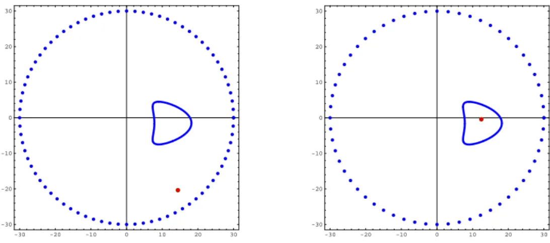
5.2.1. Example 1.
We start by studying the influence of boundary velocityg. We test two situations:
One considering boundary velocity satisfying the orthogonal condition (19) and other not satisfying this condition. The considered obstacle was the kite, defined by the parametrization
We considered Γ =∂B30(0,0) and the boundary velocitiesg1(x, y) =y⃗e1+x⃗e2
andg2(x, y) =⃗e1+⃗e2. Notice that
∫
Γ
g1·T(v1,0)ndσ=
∫
Γ
g1·T(v2,0)ndσ= 1800π
andg2satisfies the orthogonal condition (19) (see remark2). We took the measured
data at 60 observation points uniformly distributed over Γ, without adding noise. As we can see in Fig. 1 (right plot) we were able to retrieve the location of the obstacle, when the boundary velocity satisfies the orthogonal condition (19). For
this case, the retrieved location was (12,−1.5). When we considered the boundary
velocityg1 we obtained the location (12.4,−5.1), which is a bad result (see the left
plot of the mentioned figure). The results deteriorate by increasing the size of the obstacle (see Fig. 2).
-30 -20 -10 0 10 20 30
-30 -20 -10 0 10 20 30
-30 -20 -10 0 10 20 30
-30 -20 -10 0 10 20 30
Figure 1. Reconstruction results from two boundary velocities satisfying (right plot) and not satisfying (left plot) the orthogonal condition (19).
-30 -20 -10 0 10 20 30
-30 -20 -10 0 10 20 30
-30 -20 -10 0 10 20 30
-30 -20 -10 0 10 20 30
Figure 2. The same as the previous figure when considered a different size for the kite.
5.2.2. Example 2.
by γ = ∂B0.03(4.2,0) immersed in two regions: first, a region bounded by Γ =
∂B5(0,0) and then bounded by Γ =∂B30(0,0). The velocity field prescribed at Γ
wasg(x, y) =⃗e1+⃗e2.
The center was retrieved using 10, 30 and 60 observations on Γ. The numerical results are summarized in Tables 1 and 2, respectively. Overall, we obtained good reconstruction results even in the presence of noisy data.
Observations without noise 10% noise 20% noise 10 (3.02,−0.15) (3.15,−0.06) (5.33,0.17) 30 (4.18,−0.02) (5.12,0.03) (4.32,0.91) 60 (4.20007,0.00014) (4.33,0.024) (5.83,0.45) Table 1. Reconstruction of a small circular obstacleω=B0
.03(4.2,0) immersed in Ω =B5(0,0).
Observations without noise 10% noise 20% noise 10 (4.19,0.004) (3.97,0.23) (4.74,0.66) 30 (4.19,0.0003) (3.54,0.09) (4.36,0.14) 60 (4.20,0.0003) (4.26,0.19) (4.201,0.06) Table 2. The same as the previous Table but considering the domain Ω =B30(0,0).
Next, we considered several star shaped obstacles with different geometries and
locations. The boundary velocity wasg=⃗e2 for the first example and g=⃗e1+⃗e2
for the others. We took 10 noise free boundary measurements and obtained the results presented in Fig. 3. Notice that the last obstacle (plot (d) of Fig. 3) is not symmetric. The parametrization of the corresponding boundary is
γ(t) =(0.4(1.5−sin(t) cos(2t)3) cos(t) + 2)⃗e1+
(
(2.5−cos(t)3) sin(t)−0.7)⃗e2.
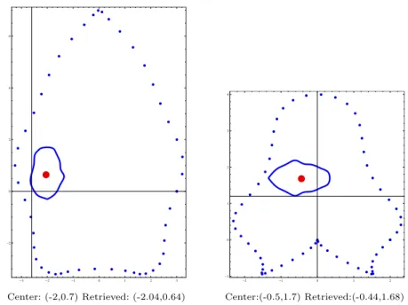
5.2.3. Example 3.
In this example we considered two different geometries for the enclosing domain Ω. In both cases, the domains are star shaped and non convex (see Fig. 4). The
boundary velocity wasg=⃗e1+⃗e2 and the noise free measured data was obtained
at 50 observation points. As we can see in Fig. 4, the location of the obstacle was retrieved accurately.
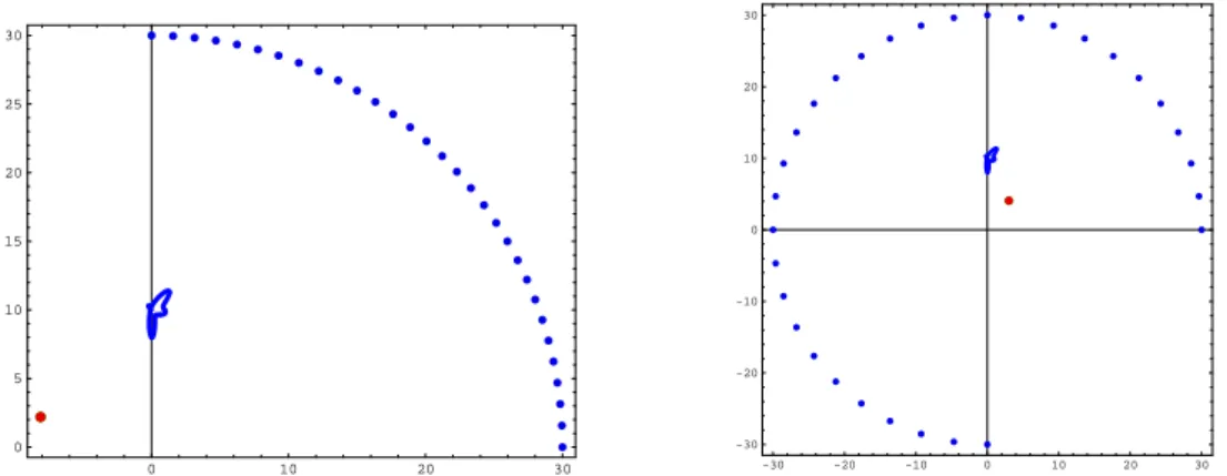
Last simulations concerns a non convex shark shaped obstacle. The boundary is given by the parametrization
γ(t) = (
1.91 + 0.9 cos (t) + 0.1 sin (2t)
1 + 0.75 sin(t) cos (4t) cos(t)−5.5 )
⃗e1
+ (
1.91 + 0.9 cos (t) + 0.1 sin (2t)
1 + 0.75 sin(t) cos (4t) sin(t)−12.7 )
⃗e2
and the enclosing domain Ω is the open ball of radius 30 centered at the origin.
The velocity considered wasg(x, y) =⃗e1+⃗e2 and we obtained the corresponding
(noise free) measurement and 10 observation points (see Fig. 5 for the reconstruc-tion results). Other locareconstruc-tion and dimension for the shark was also considered (Fig 6). Moreover, we tested for noisy data and obtained good reconstruction results.
-4 -2 0 2 4 -4
-2 0 2 4
-4 -2 0 2 4
-4 -2 0 2 4
(a) Center: (-2,1) Retrieved: (-2.13,0.97) (b) Center:(0,0) Retrieved:(-0.002,-0.00025)
-4 -2 0 2 4
-4 -2 0 2 4
-4 -2 0 2 4
-4 -2 0 2 4
(c) Center: (-2.8,1.5) Retrieved: (-2.72,1.5) (d) Center:(2.46,-0.69) Retrieved:(2.58,-0.51)
Figure 3. Reconstruction results considering 10 boundary observations and several obstacle shape and location.
second and third quadrants is illustrated by right plot of Fig. 7. In both cases, the results were not good and an a priori data completion method is required.
6. Conclusions
In this paper we proposed a reconstruction method for the location of a single 2D obstacle in a Stokes flow, using the so called reciprocity gap functional. The method is sufficiently general and can be easily adapted for 3D problems and other type of inverse obstacle problems. It is very fast and the numerical simulations shows that is accurate and stable. The good performance of the method can be exploited in, for instance, inverse geometric problems, where the geometry of the obstacle is also the goal. These problems are usually tackled as an optimization problem for both shape and location (eg. [5]). However, a more direct approach can be applied when the location of the obstacle is known (eg. [15]).
As seen in the last couple simulations, it requires data on the whole Γ, which can be a drawback.
References
-3 -2 -1 0 1 2 3 -2
0 2 4 6
-2 -1 0 1 2
-1 0 1 2 3 4
Center: (-2,0.7) Retrieved: (-2.04,0.64) Center:(-0.5,1.7) Retrieved:(-0.44,1.68)
Figure 4. Two different schemes for the observation points.
-30 -20 -10 0 10 20 30
-20 -10 0 10 20
-5 -4 -3 -2 -1
-20 -18 -16 -14 -12 -10
Figure 5. Localization of a shark. On the left, a plot of the obstacle, observation points and detected location (red bold dot). On the right, a plot of the obstacle and the retrieved location, (−5.1,−14.4).
[2] C. Alvarez, C. Conca, L. Friz, O. Kavian and J. H. Ortega,Identification of immersed obstacles via boundary measurements, Inverse Problems 21 (2005), 1531–1552.
[3] F. Caubet and M. Dambrine,Localization of small obstacles in Stokes flow, Inverse Problems 28, N. 10 (2012), 105007.
[4] C. J. S. Alves, R. Kress and A. L. Silvestre,Integral equations for an inverse boundary value problem for the two-dimensions Stokes equations, J. Inverse and Ill posed Probl. 15(5) (2007), 461 – 481. [5] N. F. M. Martins and A. L. Silvestre,An iterative MFS approach for the detection of immersed
obstacles, Engineering Analysis with Boundary Elements 32 (2008), 517–524.
[6] A. Karageorghis and D. Lesnic,The pressure-stream function MFS formulation for the detection of an obstacle immersed in a two-dimensional Stokes flow, Adv. Appl. Math. Mech., 2(2010), 183–199. [7] C. J. S. Alves and A.L. Silvestre,On the determination of point-forces on a Stokes system,
Mathe-matics and Computers in Simulation 66, issues 4–5 (2004), 385–397.
[8] C. J. S. Alves and N. F. M. Martins, Reconstruction of inclusions or cavities in potential problems using the MFS, The Method of Fundamental Solutions- A Meshless Method (Eds: C. Chen, A. Kara-georghis and Y. Smyrlis), Dynamic Publishers Inc., 2008, 51–71.
[9] S. Talbott and H. Spring,Thermal imaging of circular inclusions within a two dimensional region, Department of Mathematics, Rose-Hulman Institute of Technology (2005).
[10] N. F. M. Martins and David Soares,Localiza¸c˜ao de obst´aculos submersos a partir de dados na fron-teira, Conf. Jornadas do Mar, Escola Naval, 12-16 November 2012, Portugal.
-30 -20 -10 0 10 20 30 -20
-10 0 10 20
-0.25 0.25 0.5 0.75 1 1.25 8.5
9 9.5 10 10.5 11
Figure 6. Localization of a smaller shark. The retrieved location was (0.15,9.33).
0 10 20 30
0 5 10 15 20 25 30
-30 -20 -10 0 10 20 30
-30 -20 -10 0 10 20 30
Figure 7. Reconstruction from partial data. The obtained points are (3.03,4.07) on the right, and (8.1,2.2) on the left.
[12] L. C. Evans, Partial Differential Equations, Graduate Studies in Mathematics Vol. 19, American Mathematical Society, (1998).
[13] A. Bogomolny,Fundamental solutions method for elliptic boundary value problems, SIAM J. Numer. Anal. 22 (1985) 644–669.
[14] C. J. S. Alves and A. L. Silvestre,Density results using Stokeslets and a method of fundamental solutions for the Stokes equations, Engineering Analysis with Boundary Elements 28 (2004), 1245– 1252.