Sensitivity analysis of 3D frictional contact with BEM using
complex-step differentiation
Abstract
This paper presents a study of the complex step differentiation method applied to a parameter sensitivity analysis for 3D elastic contact problem. The analysis is performed with the Boundary Element Method (BEM) using discontinuous elements and the Generalized Newton Method with line search (GNMls). A standard BEM implementation is used and the contact restrictions are fulfilled through the augmented Lagrangian method. This methodology in conjunction with the BEM avoids the calculation of the nonlinear derivatives during the solution process, allowing a fast and reliable solution procedure. The parameter sensitivity is evaluated using complex-step differentiation. This well-known method approximates the derivative of a function analogously to the standard finite differences method, with the advantages of being numerically exact and nearly insensitive to the step-size. As an example, a Hertz-type problem is solved and the sensitivity of the contact pressures with respect to the Young Modulus variation is evaluated. The obtained results are compared with analytical and numerical solutions found in the literature.
Keywords
boundary element method, frictional contact, complex step method, sensitivity analysis.
1 INTRODUCTION
Contact problems are often found in engineering applications. While some cases can be simplified or even assumed to be irrelevant, there are others where the contact itself is the reason of the engineering problem. Wear, tear, fatigue, friction, among others, are all problems which arise as a consequence of the contact occurrence. Advanced and high performance materials, which are widely used in engineering, increase the need to predict the contact conditions as well as the mechanical response, both locally and globally.
Contact problems are often found in engineering applications. While some cases can be simplified or even assumed to be irrelevant, there are others where the contact itself is the reason of the engineering problem. Wear, tear, fatigue, friction, among others, are all problems which arise as a consequence of the contact occurrence. Advanced and high performance materials, which are widely used in engineering, increase the need to predict the contact conditions as well as the mechanical response, both locally and globally.
Unilateral contact imposes an ambiguous boundary condition, where the contact area and hence the equilibrium configuration, may have a nonlinear dependency on the loads acting on the structure. Since the works published by Fichera (1963, 1973), the contact between two solids is also known as the Signorini problem. The author obtained analytical solutions for an elastic sphere lying on a rigid plane, with and without friction, considering gravitational loads. Alart and Curnier (1991) state that the frictional contact problem is governed by a multi-valued tribological law which does not derive from a natural potential and therefore cannot be formulated as standard optimization problems using inequality constraints.
The Boundary Element Method (BEM) is well-known for its ability to solve contact problems, since its formulation intrinsically treats the displacements and tractions with same order of approximation. This enables the direct application of the contact constraints without the need of penalty parameters or Lagrange multipliers. Since the pioneer work of Andersson (1981), which used this property to develop an incremental loading technique to solve 2D contact problems, few other works are also found on the literature using the same principles, such as Paris and Garrido (1989), Garrido et al. (1991), Man et al. (1993a), Man et al. (1993b), Paris et
C.J.B. Ubessia* R. J. Marczaka
a Departamento de Engenharia Mecânica,
Universidade Federal do Rio Grande do Sul, - Porto Alegre, Rio Grande do Sul, Brasil. E-mail: [email protected],
*Corresponding author
http://dx.doi.org/10.1590/1679-78254334
al. (1995) and Garrido and Lorenzana (1998). An iterative procedure similar a predictor-corrector algorithm was used by Ghaderi-Panah and Fenner (1998). Other works using the Lagrange multiplier or the penalty parameter methods, which are mandatory for the Finite Element Method (FEM), are found in Gakwaya et al. (1992) and Yamazaki et al. (1994).
González et al. (2008) and Rodríguez-Tembleque and Abascal (2010) treated FEM-BEM coupled problems using the Augmented Lagrangian formulation to avoid some drawbacks of Lagrange multiplier and penalty methods. These approaches were based on the work of Alart and Curnier (1991). The contact restrictions are imposed in the form of projection functions, resulting in a very robust framework to both FEM and BEM frictional contact analysis. The nonlinear system of equations is then solved by the Generalized Newton Method with line search (GNMls) (Pang, 1990): a generalization of the standard Newton method to B-differentiable functions whose convergence is independent of the penalization parameter used. With an unconstrained optimization between each step of the Newton method it is also possible to accelerate the convergence. The method was also used by Rodriguez-Tembleque et al. (2011) to study 3D frictional contact on anisotropic media using the BEM. Among the existing contact treatment techniques, the Augmented Lagrangian is the most adequate in conjunction with BEM because it eliminates the need of trial and error contact state estimations (Rodríguez-Tembleque et al., 2008). This method imposes the contact restrictions exactly and treats the stick case like a standard two-region BEM formulation.
The idea of numerical differentiation by the complex step method (CSM) is due to Lyness and Moler (1967). Later, Squire and Trapp (1998) proved that if the increment is performed on the imaginary part, the resulting variation on the complex part of the function exactly approximates its derivative at that point. This avoids the evaluation of the function at two points as in finite differences. Another feature related to the use of complex variable is that the derivative is nearly independent of the increment size, which avoids common instabilities regarding the selection of this parameter. In Martins et al. (2003) an example is presented for the function
3 3
( ) = x / ( sin( ) cos( ))
f x e x x where the relative error for the derivative value is very stable and close to the
mantissa for increments of 1 10 9 to 1 10 300.
To the best of the author’s knowledge, the first application of the complex step method with BEM found on the literature is in Gao et al. (2002). It was used to obtain the stresses at internal points, avoiding the use of integral equations for stresses. Among other works, the methodology was used by Mundstock and Marczak (2009) to evaluate sensitivities in shape optimization problems, obtaining excellent results in comparison to analytical solutions.
This work describes a study of sensitivity in contact problems, applying the Complex Step Method with BEM. The paper is organized as follows. First, the contact problem is described along with the restrictions imposed. The boundary integral formulation leading to BEM equations is then presented. Next, the contact variables on the discrete form, the projection functions and the augmented variables are shown. The nonlinear system of equations is presented in a way similar to problems containing multiple regions. The GNMls and the Complex Step Method are also detailed. Results for a classical Hertz problem considering friction is solved and the results obtained are compared with its analytical solution and a previous work from the literature. The sensitivity of the contact pressure is analyzed as an application example and compared to the associated analytical derivative.
2 FORMULATION OF THE CONTACT PROBLEM
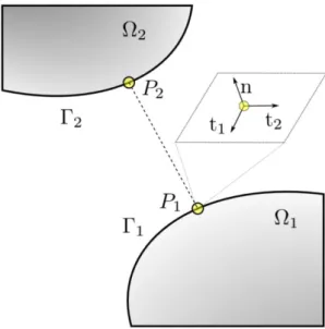
Let the problem of two elastic bodies
1 and
2, with boundary = p u c (disjoint set), where
p,
u,
c, correspond to the portion of the boundary prescribed with tractions, displacements and possible contactinterface, respectively, as illustrated in Fig. 1. As a boundary value problem, or the prescribed tractions,
p
, or the prescribed displacements,u
, are specified along the boundaries, and the complementary variables, u andp
,Figure 1: Solids under contact and boundary conditions.
The possible contact boundary have conditions which depends on the contact state, defined by the gap between the two regions. When the gap positive, the surfaces are free and the tractions are null. Compatibility conditions must be forced when the gap aperture is zero and the tractions are not null, and they depend on the existence of friction or not.
2.1 Kinematic conditions
In this work, the BEM formulation assumes small strains and infinitesimal displacements and the contact regions are treated as a node-to-node contact. The nodes are positioned in a conforming scheme, as done in Rodríguez-Tembleque et al. (2008), forming pairs, i.e., the slave nodes (the ones which belong to region
2) are positioned as closely as possible to the master (region
1) nodes, or at least matching the displacement path performed by the contact node pair. The contact variables in the discrete form are then related to the possible contact node pairs, as in Fig. 2.Figure 2: Master (
P
1) and slave (P
2) nodes along a contact interface.The gap
g
for any pair of points in this problem is obtained through the following relation2 1 2 1
(
)
(
),
T T
g B x
x
B u
u
(1)where
x
1 andx
2are coordinates on boundaries and respectively, while and are the displacements of these points, both referring to a global coordinate system. is the rotation matrix responsible for changing the variables to the local coordinate system with origin at, i.e.,1 2 ,
where n is the outward normal vector at
x
1 andt t
1 2,
are the tangential vectors. Therefore the gap can bedecomposed in its tangential and normal components:
1 2
gt gt g .n
g (3)
2.2 Unilateral and frictional contact conditions
The unilateral and frictional laws for a boundary point are grouped as suggested in González et. al. (2008), resulting in the well-known contact conditions which depends on the normal gap
g
n, normal( )
t
n and tangential( )
t
t tractions,t 0; g 0; 0; No contact case,
t 0; g 0; ; . ; Contact - Slip case,
t 0; g 0; 0; Contact - Stick case.
n n t
n n t n t t t t
n n t
t
t
t g t g t
g
(4)
The time rate in equation (4) must be approximated by a finite differences scheme. Rodríguez-Tembleque and Abascal (2010) suggested the following approximation for
g
t at time
kas. t
t
g
g (5)
2 BOUNDARY ELEMENT METHOD FORMULATION
The displacement boundary integral equation for a point in the boundary is
* = * ,
i i
lk k lk k lk k c u p u d u p d
(6)where the boundary is always smooth due to the use of discontinuous elements, i.e., 1 2
= i lk
c . In order to obtain a numerical solution from Eq. (6), the boundary is discretized into a finite number of elements.
The geometry is interpolated by standard shape functions written in terms of the parametric coordinates 1 2
( , )
:
ξ
=1
= ( ) ,
N
j n n n
x
x (7)
where
N
is the number of nodes of the element and
n is a vector containing the shape functions evaluated at . The variables are calculated at collocation points placed at an offset distance from the geometrical nodes. Displacements and tractions are interpolated with discontinuous interpolation functions := 1 = 1
= N ( ) ,j = N ( ) .j
n n n n
n n
u p
u ξ p ξ (8)
In the numerical implementation of this work linear (Q4) and quadratic (Q8) quadrilateral elements were used. The interpolation functions for the linear element are written in compact form as
1 1 2 2 2
1
= ( )( ), = 1 4,
4 n n
n d d d n
(9)
a
= 1 ,
100
d (10)
which reduces to the continuous functions
n whena =0
. The interpolation functions for the 8-node element are also written in compact form,1 1 2 2 1 1 2 2 3
1 1 2 2
3
1 1 2 2
( )( )( )
= = 1 4,
4
( )( )( )( )
= , = 5 8.
2 ( )
n n n n
n
n n n
d d d
n d
d d d d
n d d
(11)
Collocation for node
i
, generates the discretized form of Eq. (6): .e e e e
i i ij ij
C u H u G p (12)
Performing the collocation process over all boundary nodes results in the algebraic system of equations that leads to the BEM solution, i.e.,
= .
Hu Gp (13)
4 CONTACT PROJECTION FUNCTIONS
The formulation used for the imposition of contact restrictions was implemented according to González et. al. (2008). The handling of inequalities, typical of contact conditions, was avoided using suitable projection functions.
4.1 Unilateral and frictional contact conditions
To fulfill the non-penetration condition, the complementarity of the normal components of the gap and tractions variables are written in the following manner
t g 0,
t 0, g 0,
n n
n n
(14)
which means that not only one of the two variables must be null, whether is the normal tractions or the normal gap, but also that the gap must be no less than zero and the normal traction to be never positive. The above inequalities can be eliminated using the following projection function
( ) :v ,
(15)
projecting the variable v onto
, the admissible region of the contact normal tractions, i.e.( )v min( ,0).v
(16)
A mixed variable is now introduced, the augmented normal traction
t
n* , defined as*
g ,
n n n n
t
t
r
(17)where
r
n is a positive penalization parameter(
r
)
. The complementarity condition can then be fulfilledusing a single equation, *
( ) = 0.
n n
t t
4.2 Unilateral and frictional contact conditions
Similarly, the augmented tangential traction vector is defined as *
=
,
t t
r
t tt
t
g
(19)the gap must be
if < ,
( ) =
if ,
n
g n t n
t
t t
v v
v
e v
(20)
where
e
t=
v / v
. This function projects the variable onto the Coulomb disk,
g, of radiusg
=
t
n . Considering a plane defined by the tangential tractions,1 2
t t
t t ,
g represents admissible for the tangentialtractions under a given normal traction
t
n . The tangential contact restrictions are finally written as* ( ) = 0. t g t
t t (21)
4.3 Normal-Tangential operator
In order to combine the normal and tangential restrictions in a single statement, the normal-tangential projection function
f
is defined as
*
*
( )
( ) = ,
( )
t g f
n t
* t
t
(22)
where the region
f is the augmented friction cone, with radius (t*n) and inclination defined by the friction coefficient. The inequalities in Eq. (4) are then completely fulfilled though the following set of equations( ) = 0. f
*
t t (23)
5 CONTACT FORMULATION WITH BOUNDARY ELEMENTS
The system of linear equations (SLE) for a contact problem is assembled similarly as in multiple-region problems, resulting the system of equations,
1 1 1 1 1 1 1 1 1 1 1 1
2 2 2 2 2 1 2 1 2 2 2 2
= ,
= .
nc nc nc nc c c c c nc nc nc nc
nc nc nc nc c c c c nc nc nc nc
H u G p H u G p G p H u
H u G p H u G p G p H u (24)
where the compatibility conditions
2 1
2 1
, .
c c
c c
u u
p p (25)
must be enforced along the contacting interfaces.
5.1 Discrete contact variables
In order to write the contact tractions with a distinct symbol of the global ones and keeping consistency with the references notation, the local contact tractions for a node pair
i
are defined as
i. In this work, only BEM is used, thus there exist no requirement of using Lagrange multipliers, as one of the well-known advantages of BEM in contact problems is that the tractions are already part of the unknowns. The transformation between the element tractions and contact tractions can be accomplished using the following relations
1 1 ,
c
ji
j i
p C Λ (26)
2 2c ki ,
k i
p C Λ (27)
where ji
C is formed with the rotation matrix
B
assembled for each region .., according to the assembly incidencej
of each contact nodei
. That is, for a contact node pair I = ( , )j k in Eq. (26) and m= ( )I , we have:mI .
I
C B (28)
The discrete form of the gap
g
is now introduced using the same transformation. The kinematic relations of the possible contact region are written as2 2 1 1
( )T c ( )T c,
go
k k C u C u (29)
where
k
is the gap vector accounting for all the contact pairs. The vectork
go is the sum of the initial gap and rigid body displacements vectors.Substituting Eq. (26) and (27) in Eq. (24) and adding Eq. (29) to the SLE results
2
1 1 1 1 1 1
2 2 2 2
1
2 2
1 1 2 2
= ,
= ,
= ,
) ( )
(
nc nc c c c nc
nc nc c c c nc
T c T c
g g go
A x H u C G b
A x H u C G b
C u C u C k C k
Λ
Λ (30)
where
are the BEM nodal tractions rotated from the global to the master nodes local coordinate system. 5.2 Contact restrictionsThe discrete form of the contact restrictions can be incorporated to the SLE through the application of the projection functions on a node pair. Writing equation (23) for the discrete form of the contact tractions results in
*
( ) 0.
f
λ λ (31)
Substituting λ* λrk with r being the penalization parameters vector, the previous equation becomes
( ) 0.
f
rk
λ λ (32)
For the normal direction one writes the restriction as *
min( ,0)
0,
n n
(33)which, for the no contact case
( )
n I*
0
and by the Coulomb friction law,
t
n results in= 0, = 0.
n t
Writing the restrictions for the contact case for the tangential direction, one needs to write the restrictions separately for stick and slip. Along the normal direction ( ) < 0*
n I
, so the restriction equation of a node pair
I
, for both stick and slip cases, is written asmin( ,0) = 0,
n n r kn n
(35)
which leads to
= 0.
n n
r k (36)
For the stick case
(
t*) <
I
n (the first case of equation (20)), the tangential restriction results( ) 0,
g
t t rt t
λ λ k (37)
which, using
g( ) =
v v
, reads0.
t t
rk (38)
As for the slip case,
( )
t I*
n (second case of equation (20)),
f( )
λ
t*
t
n( )
e
t* , is used, so the tangential restriction is expressed as1 1 2 2 * * 0, 0,
t t n
t t n
e e
(39)
where * * * . t t t λ e
λ (40)
Grouping Eqs. (34), (36), (38) and (39), in a single system for all contact restrictions, leads to
g ,
P Λ P k= 0 (41)
where P and Pg are assembled according to the contact state of each pair
I
and depend on the contact pair state (Rodríguez-Tembleque and Abascal, 2010):• No contact case:
n I* 0g
1 0 0 0 0 0 ( ) = 0 1 0 ,( ) = 0 0 0 .
0 0 1 0 0 0
I I
P P (42)
• Stick case:
n I* < 0 andλ
*t<
nI*g
0 0 0 0 0
( ) = 0 0 0 ,( ) = 0 0 . 0 0 0 0 0
t
I I t
n r r r
P P (43)
• Slip case:
nI*< 0
and
t I*<
nI** 1 *
g 2
1 0 0 0 0
( ) = 0 1 ,( ) = 0 0 0 .
0 0
0 0 0
t
I t I
n e e r
5.3 Contact restrictions
After incorporating the contact restrictions Eq. (41), Eq. (30) can be recast as a system of the type
Rz f
=
:
1
1 1 1 1 1
2 2 2 2 2
2
1
2
1 2
go
g
( ) ( )
nc
nc c c c nc
nc c c nc nc
c
T T
x
A H 0 0 C G 0 u b
0 0 A H C G 0 x b
k
0 C 0 C 0 I u
0
0 0 0 0 P P Λ
k
(45)
where
A
nc are the columns from H or G (Eq. (24)) corresponding to the independent unknownsnc
x
for the region. c
H
are the matrices relative to the unknown tractions on the possible contact regions. The contact tractions (Λ
), as well as the gap (k
), are assumed in their local coordinate system, by the incorporation of the rotation matrices on the system of equations, i.e., Eq. (2), which are assembled for each contact pair on the main rotation matrix presented as C in Eq. (45).I
is the identity matrix and the vectorgo
k accumulates the initial gap and rigid body displacements.
6 NONLINEAR SYSTEM SOLUTION: GENERALIZED NEWTON METHOD WITH LINE SEARCH
As suggested in Rodríguez-Tembleque and Abascal (2010), the nonlinear system of equations is solved using the Generalized Newton Method with line search, first proposed by Pang (1990). The
-differentiable functions are described as non Fréchet-differentiable due mainly to the absence of linearity on the
-derivative. Pang (1990) presents an example of complementarity function H:n n, H x( ) = min( ( ), ( ))h x f x , which is nonFréchet-differentiable, the same case as the normal projection operator. Contrary to the Uzawa method, the GNMls does not require damping or stabilization parameters and its convergence is independent of the penalization factor used in the augmented Lagrangian (Alart and Curnier, 1991). Denoting the current iteration by the superscript ( )n , the GNMls algorithm can be summarized in the following steps:
1. Let z(0) be an arbitrary initial vector, and
( ) ( ) ( )
( n ) n n
Θ z R z f (46)
2. Given z( )n with Q(z( )n ) 0, the direction z( )n is obtained by solving the equation:
( ) ( ) ( )
( n ) ( n , n ) 0
Θ z Θ z z (47)
3. Find the first integer m= 1,2, which fulfills the decreasing error condition:
( ) ( ) ( ) 1 2 ( ) ( ) ,
(
n
n n) (
n) ( )
nΨ z z Ψ z
with ( )n = .qm, q> 0, (0,1), (0,1/ 2), and
2
( ) 1 ( ) .( )
2
( )
n nΨ z Θ z (48)
4. Updated solution vector: z( 1)n = z( )n ( )nz( )n
5. If ( 1) 1
( n )
Ψ z , stop. Otherwise
n n
=
1
, and return to step 2.6.1 Search direction: Directional derivatives
The system of equations (46) can be split in its linear and nonlinear parts,
( ) ( ) ( )
( n ) ( n ) ( n ), L D N L D
where ( ( )n )
LD
Θ z is the part which has the linear directional derivative at all points, and ( ( )n )
N L D
Θ z has the nonlinear derivative at some points. The
-derivative Θ z( ( )n ,z( )n ) can be separated in the same manner:
( ) ( ) ( ) ( ) ( )
( ,
n n)
( )
n( )
n n,
LD NLD
Θ z
z
Θ z
Θ
z
Δ z
(50)where ( ( )n ) LD
Θ z is the linear part of the Jacobian matrix,
1 1 1
2 2 2
1 2 ( ) 1 2 ( ) , ( ) ( )
nc c c
nc c c
n LD T T
A H 0 0 C G 0
0 0 A H C G 0
Θ z
0 C 0 C 0 I
0 0 0 0 0 0
(51)
and ( ( )n ) N L D
Θ z is the nonlinear part of the Jacobian. A linear approximation for this derivative can be used (Strömberg, 1997): ( ) ( ) ( ) , n n NLD g
0 0 0 0 0 0 0 0 0 0 0 0
Θ z 0 0 0 0 0 0
0 0 0 0 J J
(52)
where ( )n
J and ( )n
J are written for each contact pair, as are the matrices P and Pg:
• No contact case:
nI*
0
g
1 0 0 0 0 0
( ) = 0 1 0 , ( ) = 0 0 0 .
0 0 1 0 0 0
I I I I
J J (53)
• Stick case:
nI*< 0
and
t I*<
nI*g
0 0 0 0 0
( ) = 0 0 0 , ( ) = 0 0 .
0 0 0 0 0
t
I I t
n I I r r r
J J (54)
• Slip case:
nI*< 0
and
t I*>
nI*( ) ( )
*
11 12 1 11 12
( ) * ( )
21 22 2 g 21 22
0
( ) = , ( ) = 0 ,
0 0
0 0 0
n n
t t t
n n
I t I t t
n I I
r r
J r r
r J
(55)
where Ψ (1)I R ,Ψ Ψ I , ( * ( )n ) ( * ( )n )
t I t I
R Λ Λ , and
*( ) *( ) ( ) ( ) n n I n t I
ΛΛ , *( ) 3 *( ) ( ) ( ) n n I n t I Λ
Λ .
6.2 Linearized Derivatives
It is possible to simplify the contact nonlinear system even further by assuming that the nonlinear part of the directional derivatives ( ( )n )
I
(Rodríguez-Tembleque and Abascal, 2010). To find the iteration direction Δ z( )n , this simplification leads to the following equation to be solved:
( ) ( ) ( )
( n ) n n 0,
Θ z R Δ z (56)
which is the same as solving the following SLE,
( )n ( ( )n ( )n ) 0.
R z Δ z f (57)
7 COMPLEX STEP METHOD
Mundstock and Marczak (2009) obtained good results calculating shape derivatives for 2D elasticity problems using the complex step method with the BEM. In order to calculate the derivative of a function f x( ), one has to take the complex part of the solution and divide it by the perturbation
h
, as in2
( )= Im[ ( . )] ( ).
f x f x i h O h
x h
(58)
The procedure can be extended to evaluate any kind of derivative in existing numerical codes by adding the complex increment to the desired variable, as long as f x( ) is a real function.
8 RESULTS
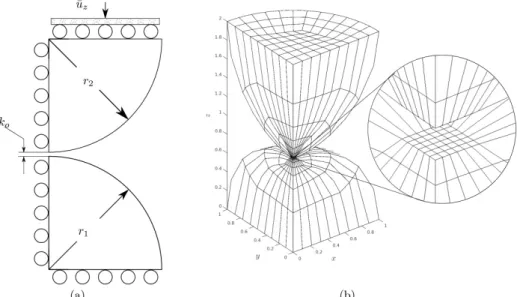
The problem analyzed in this work consists of two spheres in contact (Fig. 3a), allowing the direct comparison with the classical Hertz solution. Both solids were considered elastic which is not a case commonly seen in the literature - generally, one of the bodies is considered rigid and the other a half-space BEM region. The mesh was simplified by taking advantage of the symmetries, as shown in Fig. 3b. The discretization used allows the evaluation of the algorithm when a small region of the solid is transferring the load, resulting in significant stress concentration at a few nodes.
The mesh used for each sphere has 264 quadrilateral elements, and is illustrated in Fig. 3b for quadratic elements. The mesh has a large element size ratio in order to reduce the overall number of degrees of freedom (DOF) without compromising the solution accuracy. The linear and quadratic elements resulted in 6936 and 14400 DOF respectively. The kinematic relations and the contact restrictions accounted for 9 percent of these DOF.
Prescribed displacements uz were applied to the upper face of the half sphere, while symmetry conditions
were used over the corresponding planes.
An offset of 12.5% was used in all the elements, and all material and geometrical properties considered are listed in Table 1. To the best of authors knowledge there is no closed form solution for this problem when 0. In order to provide a reference solution for comparison of the results, the geometrical and material properties selected were the same as in Rodríguez-Tembleque and Abascal (2010). The friction coefficient used was = 0.1. Table 1 also lists the maximum contact pressure p0 and the contact area radius predicted for the prescribed displacements uz, from Johnson (1987).
Table 1: Sphere on Sphere contact problem parameters and results from the hertz solution.
BEM model parameters
Young's Modulus (both spheres) E1 E2 1e4 Pa
Poisson Ratio (sphere 1) 1 0.3 -
Poisson Ratio (sphere 2) 2 0.4 -
Coulomb friction coefficient
0.1 -Radius (both spheres) R1 R2 1.0 m
Initial Separation k0 1.0E-1 m
final stress (MPa) uz k0 8.0E-4 m
Hertz solution Maximum contact presure (Eq.(60)
0
p
145.5161 PaRadius of the contact area a 2.0E-2 m
A single load step was used to set the boundary conditions, and the initial parameters for the GNMls were = 1.0
q , = 0.90, rt = rn = 0.70. The residue Ψ( )n and the scaling parameter ( )n during the GNMls iterations
are shown in Fig. 4. The residue during the first iterations does not change, i.e., once the algorithm finds an optimal direction, it converges with a logarithmic rate.
Figure 4: (a) GNMls convergence: Residue (Ψ( )n ) and scaling parameter (( )n ) obtained by the line search procedure
for each iteration (n).
The displacements along the contact area are plotted in Fig. 5, as a function of the coordinates x. These
values were extracted from a line of nodes close to plane of symmetry x z . Both numerical and analytical
displacements were normalized with the prescribed displacements uz. In this particular example, the quadratic
The tangential slip obtained for both elements is also depicted in the figure, normalized with respect to the maximum slip of the quadratic element. In this case it is possible to verify the transition from stick to slip states.
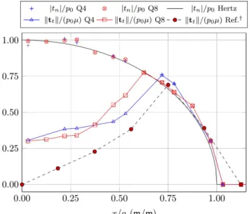
Figure 6 shows the normal contact tractions n normalized with the maximum analytic pressure p0. The normal displacements and tractions agree well with the reference solution. The norm of tangential tractions divided by the friction coefficient is also plotted.
At approximately 75% of the normalized contact distance the tangential traction reach the maximum value predicted by the Coulomb law, precisely where the nodes initiate the slip state. Although the maximum normal traction does not present a pronounced difference between the linear and quadratic elements, at the tangential direction it is possible to see a larger difference between the two. The quadratic elements also predict a larger slip region. At this transition region the normal tractions are in much better agreement with the reference solution, what indicates a better approximation by the quadratic element. This effect is also noted in the results of Rodríguez-Tembleque and Abascal (2010), as the number of nodes is even more reduced in their mesh. The tangential tractions should have vanished at the symmetry line
x
= 0
, but they are producing a residual value. In numerical experiments we found out that if entire meshes are used without the aid of symmetry, correct values are obtained.Figure 5: Normalized displacements and tangential slip along possible contact region.
8.1 Sensitivity analysis
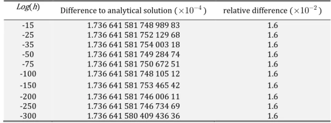
The initial analysis for any finite difference scheme should be a verification of step size. However, in order to show the independence of complex step method with respect to the step size, a variation ranging from 1e-15 to 1e-300 was tested.
The complex step was added to the value of the elastic modulus used in the top sphere, and the maximum contact pressure sensitivity was analyzed. The comparison was carried out against the analytical solution, obtained by deriving the Hertz equation for pressure with respect to E1.
Due to the position of the collocation points in discontinuous elements, there is no node exactly at
x
= 0
, so the analytical solution was evaluated at the position of the closest node.According to Johnson (1987), the normal pressure distribution along the contact region is given by: 2
0 2
( ) =
1
r
,
p r
p
a
(59)where po is the maximum pressure and r is the distance from the center of the sphere. po is related to the
material and geometrical properties by the equation
* *
0= 2 ( /0 ),
p E u R (60)
where u0 is the prescribed displacement, R* = (1 / R1 1 / R2)1 and E* is the equivalent elastic modulus of the
pair:
* 2 2 1
1 1 2 2
= ((1 ) / (1 ) / ) .
E E E (61)
Considering 1= 2 = , the result for the derivative of the maximum pressure is
2
o 1
2
2 2
1 2 1 2
1
1 2
(2/ ) (u / R) 1
= .
1 1
o
p E
E
E E
(62)
The pressure sensitivity is therefore 2
2 1 1
=
p
o1
p
r
E
E
a
(63)Eq. (63) results, for r = 6.3 10 4m, a sensitivity of 7.56 10 3. Table 2 shows the difference obtained by the present approach to the analytical solution, for different values of complex increments. As can be seen, the actual difference is larger than the variation of the results, revealing stability of the method for any step size chosen.
Table 2: Difference of the numerical solution to the analytic values of Eq. (63) – element Q8. Log(h) Difference to analytical solution (104) relative difference (102)
-15 1.736 641 581 748 989 83 1.6
-25 1.736 641 581 752 129 68 1.6
-35 1.736 641 581 754 003 18 1.6
-50 1.736 641 581 749 284 74 1.6
-75 1.736 641 581 750 672 51 1.6
-100 1.736 641 581 748 105 12 1.6
-150 1.736 641 581 753 465 42 1.6
-200 1.736 641 581 746 006 11 1.6
-250 1.736 641 581 746 734 69 1.6
Figure 7 illustrates the normal and tangential traction sensitivities over the contact area. It is worth to note traction shows the higher sensitivity, differently from Fig. 6, where they were divided by the friction coefficient.
Figure 7: Sensitivity of normal and tangent contact tractions to the variation of
E
18.1 Computational Aspects
The code was developed under Matlab environment. All computations were performed on a Desktop PC running Linux OS. The maximum memory usage was approximately 5 Gb during assembly procedures, reducing to 1.7 Gb during the solution process, for quadratic elements. The system size was small enough to fit on the system's RAM, allowing the use of UMFPACK direct solver from Davis (2004). The total run time for the cases using complex algebra was 600 seconds, while the non complex time was around 300 seconds.
Preliminary tests suggests avoiding iterative solvers whenever possible due to their need of efficient preconditioning schemes. The iterative solvers tested (GMRES, BICG and other variants) needed a considerable number of iterations, related to the poor matrix conditioning, resulting in a longer solution time. Even with the lower operation complexity of iterative solvers, the poor floating point per second performance of the sparse matrix-vector operations, when compared with the BLAS3 routines used by the UMFPACK direct solver, resulted in a longer solution time. Investigations on iterative solvers with BEM found on Barra et al. (1992), Valente and Pina (2006), Xiao and Chen (2007), also show a large number of iterations.
9 CONCLUSIONS
This work evaluated the use of complex step method to obtain sensitivities on BEM-BEM contact problems with friction. For the particular case evaluated, the nonlinear solution obtained by the GNMls presented a fast convergence.
Despite all the simplifications considered, the results obtained for the normal direction of displacements and tractions on the contact regions have shown a relative difference to the analytical solution of 1 10 2. Moreover, the tangential tractions appear to be more affected by such simplifications, as can be seen in the non vanishing tangential tractions at center of the contact. This result is also affected by the symmetry boundary condition in conjunction with the use of discontinuous elements.
The numerical sensitivities evaluated with present scheme also agreed well with the reference solution, making the present approach a potential candidate to be implemented in structural optimization cases containing contact.
The run times indicate that the complex variables do not affect the integration, assembly, or the solution performance more than the additional time needed to handle double data sizem, if compared to a standard BEM code.
It is also important to point out that the complex increment stands as an optimum scheme to be used in other contact problems since it does not affect the contact state when it is added to the nodal positions, and has proven to be very stable and reliable, regardless the step size. This robustness more than compensates its two-fold memory requirements and solution time.
10 ACKNOWLEDGEMENTS
The authors wish to express his thanks to CNPq for the financial support.
References
Alart P., Curnier A. (1991) A mixed formulation for frictional contact problems prone to newton like solution methods, Comput. Methods Appl. Mech. Eng. 92(3): 353–375.
Andersson T. (1981) The boundary element method applied to two-dimensional contact problems with friction, in ‘Boundary element methods’, Springer, pp. 239–258.
Barra L., Coutinho A., Mansur W., Telles J. (1992) Iterative solution of bem equations by gmres algorithm, Computers & Structures 44(6): 1249 – 1253.
Davis T. A. (2004) Algorithm 832: Umfpack v4.3—an unsymmetric-pattern multifrontal method, ACM Trans. Math. Softw. 30(2): 196–199.
Fichera G. (1963) Sul problema elastostatico di Signorini con ambigue condizioni al contorno., Atti Accad. Naz. Lincei, VIII. Ser., Rend., Cl. Sci. Fis. Mat. Nat. 34: 138–142.
Fichera G. (1973) Boundary value problems of elasticity with unilateral constraints, in ‘Linear Theories of Elasticity and Thermoelasticity’, Springer, pp. 391–424.
Gakwaya A., Lambert D., Cardou A. (1992) A boundary element and mathematical programming approach for frictional contact problems, Computers & Structures 42(3): 341 – 353.
Gao X., Liu D., Chen P. (2002) Internal stresses in inelastic BEM using complex-variable differentiation, Computational Mechanics 28(1): 40–46.
Garrido J., Foces A., Paris F. (1991) BEM applied to receding contact problems with friction, Mathematical and Computer Modelling 15(3): 143–153.
Garrido J., Lorenzana A. (1998) Receding contact problem involving large displacements using the BEM, Engineering Analysis with Boundary Elements 21(4): 295 – 303. Contact Mechanics.
Ghaderi-Panah A., Fenner R. (1998) A general boundary element method approach to the solution of three-dimensional frictionless contact problems, Engineering Analysis with Boundary Elements 21(4): 305 – 316.
Johnson K. L. (1987) Contact mechanics, Cambridge university press.
Lyness J. N., Moler C. B. (1967) Numerical differentiation of analytic functions, SIAM Journal on Numerical Analysis 4(2):202–210.
Man K., Aliabadi M., Rooke D. (1993a) BEM frictional contact analysis: load incremental technique, Computers & structures 47(6):893–905.
Man K., Aliabadi M., Rooke D. (1993b) BEM frictional contact analysis: modeling considerations, Engineering analysis with boundary elements 11(1):77–85.
Martins J. R., Sturdza P., Alonso J. J. (2003) The complex-step derivative approximation, ACM Transactions on Mathematical Software (TOMS) 29(3):245–262.
Mundstock D. C., Marczak R. J. (2009) Boundary element sensitivity evaluation for elasticity problems using complex variable method, Structural and Multidisciplinary Optimization 38(4):423–428.
Pang J.-S. (1990) Newton’s method for b-differentiable equations, Mathematics of Operations Research 15(2):311–341.
Paris F., Blazquez A., Canas J. (1995) Contact problems with nonconforming discretizations using boundary element method, Computers & structures 57(5): 829–839.
Paris F., Garrido J. (1989) An incremental procedure for friction contact problems with the boundary element method, Engineering Analysis with Boundary Elements 6(4): 202 – 213.
Rodríguez-Tembleque L., Abascal R. (2010) A FEM-BEM fast methodology for 3d frictional contact problems, Computers and Structures. 88(15-16): 924–937.
Rodriguez-Tembleque L., Buroni F., Abascal R., Sáez A. (2011) 3d frictional contact of anisotropic solids using bem, European Journal of Mechanics-A/Solids 30(2): 95–104.
Rodríguez-Tembleque L., González J. A., Abascal R. (2008) A formulation based on the localized Lagrange multipliers for solving 3D frictional contact problems using the BEM, Numerical Modeling of Coupled Phenomena in Science and Engineering: Practical Use and Examples p. 359.
Squire W., Trapp G. (1998) Using complex variables to estimate derivatives of real functions, SIAM Review 40(1):110–112.
Strömberg N. (1997) An augmented Lagrangian method for fretting problems, European Journal of Mechanics-A/Solids 16, 573–593.
Valente F., Pina H. (2006) Conjugate gradient methods for three-dimensional BEM systems of equations, Engineering Analysis with Boundary Elements 30(6):441 – 449.
Xiao H., Chen Z. (2007) Numerical experiments of preconditioned krylov subspace methods solving the dense non-symmetric systems arising from bem, Engineering Analysis with Boundary Elements 31(12): 1013 – 1023.