J. Aerosp. Technol. Manag. vol.9 número3

(1)

J. Aerosp. Technol. Manag., São José dos Campos, Vol.7, No_{3, pp.287-300, Jul.-Sep., 2017} ABSTRACT: In this study conservation equations were

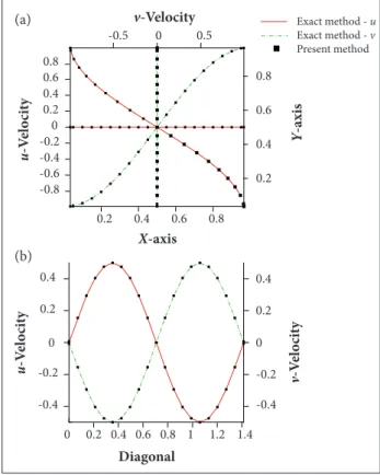
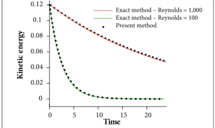
implemented along the boundaries via ghost control-volume immersed boundary method. The control-volume inite-element method was applied on a cartesian grid to simulate 2-D incompressible low. In this approach, mass and momentum equations were conserved in the whole domain including boundary control volumes by introducing ghost-control volume concept. The Taylor problem was selected to validate the present method. Four different case studies of Taylor problem encompassing both inviscid and viscous low conditions in ordinary and 45° rotated grid were used for more investigation. Comparisons were made between the results of the present method and those obtained from the exact solution. Results of the present method indicated accurate predictions of the velocity and pressure ields in midline, diagonal, and all boundaries. The agreement between the results of the present method and the exact solution was very good throughout the whole temporal domain. Furthermore, comparison of the rate of kinetic energy decay in viscous case showed same level of agreement between the results. KEYWORDS: Immersed boundary method, Control-volume-based inite element, Sub-control volumes, Conservation of mass and momentum equations, Ghost node, Ghost sub-control volume.

Immersed Boundary Method Based on the

Implementation of Conservation Equations

along the Boundary using Control-Volume

Finite-Element Scheme

Seyedeh Nasrin Hosseini1_{, Seyed Mohammad Hossein Karimian}1

INTRODUCTION

The immersed boundary method (IBM) is known as a powerful approach for simulating lows in moving boundary and complex geometry problems. In this method, discretization of equations is carried out on a Cartesian grid, which is simple to generate. However, the boundary does not conform to the grid lines, and therefore indirect methods are employed to apply the boundary conditions. his creates a range of diferent methods developed in the context of IBM which are applied to elastic (Peskin 1972, 1982; Beyer Jr 1992; Fauci and McDonald 1995; Zhu and Peskin 2003) and solid (Berger and Atosmis 1998; Khadra et al. 2000; Tseng and Ferziger 2003; Saiki and Biringen 1996) boundaries. The conventional ghost-node method is currently used in problems with solid boundaries, where the value of ghost-node is set as to meet the boundary conditions. In ghost-node methods, inite diference scheme is usually used to simulate the flow field and the value of ghost-node is determined using a kind of interpolation schemes (Mittal and Iaccarino 2005; Majumdar et al. 2001; Ghias et al. 2004; Mittal et al. 2008). While these approaches are considered fairly fast in convergence and simple in application, mass and momentum equations are not conserved in applying boundary conditions. However, the so-called cut-cell method is a complicated approach based on Cartesian grid (Clarke et al. 1986; Udaykumar et al. 2001, 1999, 1996; Ye et al. 1999), which implements conservation laws in boundary cells. In this method the shape of Cartesian cells in the vicinity of the doi: 10.5028/jatm.v9i3.672

1.amirkabir university of Technology – aerospace Engineering Department – Tehran/Tehran – Iran.

Author for correspondence:Seyed Mohammad Hossein Karimian |amirkabir university of Technology – aerospace Engineering Department | 424 Hafez ave. | 015875-4413 – Tehran/Tehran – Iran | Email: hkarim@aut.ac.ir

(2)

J. Aerosp. Technol. Manag., São José dos Campos, Vol.7, No_{3, pp.287-300, Jul.-Sep., 2017}

288 Hosseini SN, Karimian SMH

boundary is changed to i t the boundary. In cut-cell method, cells are divided by the boundary, and conservation laws are implemented in divided cells conforming to the boundary. Comparing to ghost node methods used in IBM, cut-cell method is extremely complicated. h is is because the boundary may cut the Cartesian grids anywhere on the cells and create new arbitrary shape. It would make it more diﬃ cult to discretize the equations and calculation of l uxes particularly in 2- and 3-D and moving problems.

In the present study, an immersed boundary method based on CVFE scheme is proposed in the context of ghost node concept in which conservation of conserved quantities is enforced. Importantly, the present method has the capability to conserve mass and momentum equations along the boundary. h e present approach is dif erent from the cut-cell method such that boundary cell shapes remain unchanged.

NUMERICAL ALGORITHM

h e governing equations in the present method are solved via CVFE scheme, which was presented by Minkowycz et al. (1988) to discretize governing equations. Sub-control-volume (SCV) and node types are further explained to implement boundary conditions.

CONTROL-VOLUME FINITE-ELEMENT METHOD In this scheme, solution domain is always discretized into a number of Cartesian elements. As shown in Fig. 1a, a local coordinate system (s,t) is dei ned in the middle of each element. h is local coordinate system divides each element into 4 SCVs. Each SCV is associated with an element node at its

vertex. h erefore, as shown in Fig. 1c, the grey area represents a control volume made from surrounding 4 SCVs neighbour elements. All primitive variables are located at the vertices of the elements, placing them in the middle of each control volumes. Although governing equations are finally conserved on control volumes such as the one shown in Fig. 1b, their formation are done through the assembly of elemental equations (Minkowycz et al. 1988). Elemental equations of each element include conservation of governing equations on the 4 SCVs of that element. Variables and their gradients should be evaluated at the integration points (Fig. 1a) to determine the flux at each sub-control surface. Variables with elliptic nature or of diffusion type such as pressure and diffusion can be calculated using bilinear interpolation. Minkowycz et al. (1988) presented a bilinear shape function to determine the value of variables everywhere in the element (Fig. 1a). Accordingly the value of variable φ and its gradients can be determined by:

Figure. 1. (a) Dei nitions of the element. Local coordinate system of (s,t) is located in the middle of the element, sub-control surface is indicated, and integral points are shown via cross symbols in the middle of sub-control surfaces; (b) The grey area is the SCV, and surface normal vectors are indicated in its outward direction; (c) The dark grey area in the center of the i gure is control volume made up of 4 surrounding SCVs and the light grey area is SCV.

Element 1

1 2

4 3

Node

Control volume surface Control

volume

Sub-control volume

Surface normal vectors Isolated

element

Sub-control surface 1

SCV2 SCV1

SCV3 SCV4

t = 1

t s

4 3 2

1 ×

× ×

×

t = –1

S = –1 S = 1

2

4 3

Integral point Sub-control

surface

where ϕ_i is the value of φ at the vertices of each element; N_i is the ith_{bilinear shape function.}

Modelling of other variables without elliptic nature or diffusion type such as velocity components in mass fluxes and convection terms will be discussed in more details later. Details of the CVFE method and the formation of the system of governing equation were presented by Minkowycz et al. (1988).

∑

∫ ∫ ∫

(�

� ) ( � �

� ) (

) (

)

( )

∫

∫ ∫

� _�

(� _� ) (� _� ₎

� ̂ � ̂

�

(� ̂ ) (� ̂ )

�

(� ̂ ) (� ̂ )

∫

∫ ∫

� ̂ � ̂ � ̂⃗⃗⃗⃗ ⃗⃗⃗⃗⃗⃗ ∑

∑

∫ ∫ ∫

(�

� ) ( � �

� ) (

) (

)

( )

∫

∫ ∫

� _�

(� _� ) (� _� ₎

� ̂ � ̂

�

(� ̂ ) (� ̂ )

�

(� ̂ ) (� ̂ )

∫

∫ ∫

� ̂ � ̂ � ̂⃗⃗⃗⃗ ⃗⃗⃗⃗⃗⃗

(1)

(2)

(3)

289

Immersed Boundary Method Based on the Implementation of Conservation Equations Along the Boundary Using Control-Volume Finite-Element Scheme

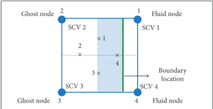
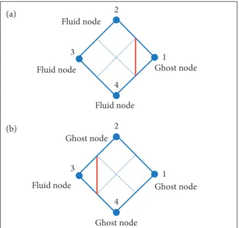
SUB-CONTROL VOLUMES AND NODE TYPES Discretization of governing equations and calculation of l uxes are done on SCVs; hence, the classii cation of dif erent sub-control volumes and nodes is described here. h ere are 4 SCVs in each element as previously explained according to Fig. 1a. Depending on the location of elements in the domain, the SCVs and nodes are classii ed into 3 types in this paper. h e i rst type of SCV is the “ordinary” or “l uid” one that is in the middle of the solution domain and it has no boundary in its SCV or in its related element (Fig. 2). An ordinary node is assigned to each related ordinary SCV. In the second type the boundary has crossed the SCV. h is type of SCV and its pertaining node are called ghost SCV type I and ghost node type I, respectively (Fig. 3). Lastly, as shown in Fig. 4, the third type is dei ned when the boundary is placed in the SCVs of l uid nodes in the element. These SCVs are called ghost SCV type II and accordingly each related node is called ghost node type II (Fig. 4). To conclude, in this method, whenever the immersed boundary is placed within an element, nodes outside of the l ow i eld are called ghost nodes (nodes 2 and 3 in Figs. 3 and 4) and their corresponding SCVs (SCVs 2 and 3 in Figs. 3 and 4) are called ghost SCVs. In this paper boundary

Figure 2. Ordinary SCV and node. all 4 SCVs and nodes are ordinary (l uid).

Figure 5. SCV and node types classii cation. SCVs and

node types

Ordinary (fluid) SCV or node

No boundary in the SCV or in its related elements

Type I Boundary has crossed the SCV

Type II Boundary is places at the SCV of fluid node Ghost

SCV or node

Ghost node 2 1

3 4

Ghost node

Fluid node

SCV 1 × 1

× 4 2

×

3 × SCV 2

SCV 4 SCV 3

Fluid node

Boundary location

Ghost node 2 1

3 4

Ghost node

Fluid node

SCV 1

× 1

× 4 2

× 3 × SCV 2

SCV 4 SCV 3

Fluid node Boundary

location

Fluid node 2 1

3 4

Fluid node

SCV 1

× 1 × 4 2

× 3 × SCV 2

SCV 4 SCV 3

Fluid node

Figure 4. Ghost SCV and node type II. The grey area indicated in SCVs 1 and 4 are ghost SCV type II related to nodes 2 and 3 (ghost nodes type II). Nodes 1 and 4 are l uid ones.

Figure 3. Ghost SCV and node type I; grey area indicated in SCVs 2 and 3 are ghost SCVs type I, nodes 1 and 4 are l uid nodes and nodes 2 and 3 are ghost node type I.

conditions are applied via ghost SCVs (Fig. 5 ). Note that SCVs of both l uid and ghost nodes are always considered as ordinary SCVs or ghost SCVs, respectively, regardless of the boundary location. As noted earlier in conventional IBMs (sharp interface methods — Seo and Mittal 2011; Ghias et al. 2007) boundary conditions are applied via the assignment of appropriate values for the l ow variables to the ghost nodes. h ese values are mostly assigned by a kind of interpolation scheme (Mittal and Iaccarino 2005; Majumdar et al. 2001; Ghias et al. 2004, 2007). In the present method, however, l ow variables on the ghost nodes are determined by implementation of conservation laws and the boundary condition on ghost SCVs. Details of the method will be discussed in following section.

GOVERNING EQUATIONS AND DISCRETIZATION In Eq. 3 there is a detail analysis of how Navier-Stokes equations were discretized. h e integral form of the incompressible Navier-Stokes equations for 2-D l ow is given by

(3)

where Q is the vector of conserved quantities; E and F are

∑

∫ ∫ ∫

(�

� ) ( � �

� ) (

) (

)

( )

∫

∫ ∫

� _�

(� _� ) (� _� ₎

� ̂ � ̂

�

(� ̂ ) (� ̂ )

�

(� ̂ ) (� ̂ )

∫

∫ ∫

� ̂ � ̂ � ̂⃗⃗⃗⃗ ⃗⃗⃗⃗⃗⃗ ∑

∑

∫ ∫ ∫

(�

� ) ( � �

� ) (

) (

)

( )

∫

∫ ∫

� _�

(� _� ) (� _� ₎

� ̂ � ̂

�

(� ̂ ) (� ̂ )

�

(� ̂ ) (� ̂ )

∫

∫ ∫

(4)

convection lux vectors; G and H are difusion lux vectors;

ν

is volume.

he extended form of these vectors is:

location, which is the ip. For the diffusion flux vectors G and H, bi-linear interpolation (Eq. 2) is used to directly evaluate the components of stress tensor (Karimian and Schneider 1994b). In the convection flux vectors E and F, pressure is evaluated using bilinear interpolation (Eq. 1), and the momentum fluxes are linearized with respect to mass fluxes and. Velocity components u and v in mass fluxes are called integral-point convecting velocities and have been previously denoted by (ρu) and (ρv) (Karimian and Schneider 1994a). Other values of u and v in the momentum fluxes, which are convected by the mass fluxes through the control-volume surfaces, are called convected velocities. Convecting and convected velocities are cell-face, which are modelled in terms of nodal values of velocity and pressure.

Karimian and Schneider (1994a) reported the implementation of the corresponding governing equations of flow to derive cell-face velocities (convected and convecting velocities) (Karimian and Schneider 1994a). In this method convected velocity is obtained from the following equation:

where ρ represents density; u and v are velocity in x and y directions, respectively; τ is shear stress; μ is viscosity; p means pressure.

Upper-case letters were used to indicate nodal values and the lower-case ones, to show the values of variables on integral points (ip). Ater substituting stress tensor within G and H, the simpliied form would be as shown in Eq. (5).

Firstly the ordinary SCV is explained. Navier-Stokes equations should be discretized in all of the four SCVs of each element in order to form element-level equations. In a case of ordinary SCV, the process of discretizing is straightforward as described in Karimian and Schneider (1994a). his process is explained in more details as follows. SCV 1 in Fig. 1a is considered here where Eq. 3 is written for this SCV as follows:

where SS stands for the inner sub-control surface shown in Fig. 1a; ds_x and ds_yare the components of normal surface vector in the outward direction.

The volume integral of the transient term is estimated using a lumped approach. Surface-integrals of E, F, G, and H are calculated by their average values over SS at the midpoint

In Eq. 7 the convection term is represented in stream wise direction and q = (u2₊_v2₎1/2_{. Expression for convected} velocity u is obtained on integration points which encompass all relevant variables related to low condition. he convecting velocity u ˆ on ip is obtained from Eq. 8 as follows:

(4)

(5)

(7)

(8)

(6)

For details about the modeling of cell-face velocities and their role in resolving pressure velocity decoupling in incompressible low, see (Karimian and Schneider 1994a).

In the current research ater completing the discretization of Navier-Stokes equations, a fully coupled algorithm is used to solve the resulted system of equations to obtain the low variables (pressure and velocity components: p, u, and v). his system of equations is solved simultaneously using a band solver.

BOUNDARY CONDITIONS AND GHOST SUB-CONTROL VOLUMES

In IBM, low variables are assigned so that their value guarantees satisfaction of boundary condition on the immersed

(5)

291

Immersed Boundary Method Based on the Implementation of Conservation Equations Along the Boundary Using Control-Volume Finite-Element Scheme

boundary. As mentioned before, in the present method l ow, variables on the ghost nodes are determined by implementation of conservation laws and the boundary condition on ghost SCVs. h erefore, the key-point in the present method is to clearly implement conservation laws on ghost SCVs along the boundaries. h is process is explained here for the ghost SCVs types one and two.

Ghost Sub-Control Volume Type I

In Fig. 6 an element with ordinary SCVs 1 and 4, and ghost SCVs 2 and 3 is presented. Implementation of Eq. 3 on ordinary SCVs 1 and 4 is done as described in previous section. h us, mass and momentum conservation equations on ordinary SCV 1 would be:

Figure 6. Ghost SCV type I (grey area in SCV 2 is considered); SSl is the left part of sub-surface 2; SS2r is the right part of sub-surface 2 along the grey area; SSb is the boundary portion in SCV 2; v2 is the volume of the grey area; dsb is normal surface vector of boundary in SCV 2 in direction to outward of the grey area; dsx2 ₁ is the normal surface vector of sub-surface1; ds_y2

2r is normal surface vector related to right part of sub-surface 2; ∆x and ∆y are grid dimensions; points 1, 2, 3, and 4 indicated with cross symbols are ip.

Ghost node 2

2 2r s t y x

b ×

1 3 4 Ghost node SSI Fluid node × 1 × 4 2 × 3 × Fluid node Boundary

location × _×

∆x ∆y v2 d sb d

sy₂2_r

d

sx₁2

where:

ν

₁ is the volume of ordinary SCV 1; the superscript “ o _{” denotes value from the previous time step; ∆t is the time}

step. Lower and upper numeric indices in the normal surface vector components, for instance ds_x2

1 , denote that dsx is

calculated on sub-surface 1 for the SCV 2. Similar equations can be obtained for other ordinary SCVs in the domain, e.g., SCV 4 in this element.

Next the implementation of Eq. 3 on ghost SCVs is explained. Ghost SCVs 2 and 3 are type I. The grey area in Fig. 6 represents the ghost SCV 2 in the flow field. This is an “effective” volume of ghost SCV 2 denoted by

ν

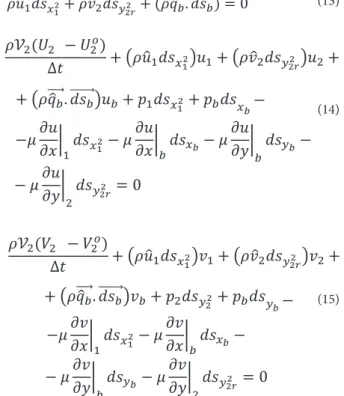
₂ this part. Substituting these parameters in Eq. 3 for SCV 2 it results in:

(9) (13) (15) (14) (10) (11)

�

(� ̂

)

(� ̂

)

(� ̂

⃗⃗⃗⃗

⃗⃗⃗⃗⃗⃗ )

_|

�

(� ̂

)

(� ̂

)

(� ̂

⃗⃗⃗⃗

⃗⃗⃗⃗⃗⃗ )

_|

� ̂

(� ̂

⃗⃗⃗⃗

)

� ̂

⃗⃗⃗⃗

� ̂

⃗⃗⃗⃗

�

(

)

(� ̂

)

(� ̂

)

(� ̂

⃗⃗⃗⃗

)

_|

�

(

)

�

(

)

(� ̂

)

(� ̂

⃗⃗⃗⃗

)

|

_|

{

�

(

)

�

(

)

} (� ̂

)

(� ̂

⃗⃗⃗⃗

)

_|

�

(

)

(� ̂

)

(� ̂

)

(� ̂

⃗⃗⃗⃗

)

_|

�

(� ̂

)

(� ̂

)

(� ̂

⃗⃗⃗⃗

⃗⃗⃗⃗⃗⃗ )

_|

�

(� ̂

)

(� ̂

)

(� ̂

⃗⃗⃗⃗

⃗⃗⃗⃗⃗⃗ )

_|

� ̂

(� ̂

⃗⃗⃗⃗

)

� ̂

⃗⃗⃗⃗

� ̂

⃗⃗⃗⃗

�

(

)

(� ̂

)

(� ̂

)

(� ̂

⃗⃗⃗⃗

)

_|

�

(

)

�

(

)

(� ̂

)

(� ̂

⃗⃗⃗⃗

)

|

_|

{

�

(

)

�

(

)

} (� ̂

)

(� ̂

⃗⃗⃗⃗

)

_|

�

(

)

(� ̂

)

(� ̂

)

(� ̂

⃗⃗⃗⃗

)

_|

�

(� ̂

)

(� ̂

)

(� ̂

⃗⃗⃗⃗

⃗⃗⃗⃗⃗⃗ )

_|

�

(� ̂

)

(� ̂

)

(� ̂

⃗⃗⃗⃗

⃗⃗⃗⃗⃗⃗ )

_|

� ̂

(� ̂

⃗⃗⃗⃗

)

� ̂

⃗⃗⃗⃗

� ̂

⃗⃗⃗⃗

�

(

)

(� ̂

)

(� ̂

)

(� ̂

⃗⃗⃗⃗

)

_|

�

(

)

�

(

)

(� ̂

)

(� ̂

⃗⃗⃗⃗

)

|

_|

{

�

(

)

�

(

)

} (� ̂

)

(� ̂

⃗⃗⃗⃗

)

_|

�

(

)

(� ̂

)

(� ̂

)

(� ̂

⃗⃗⃗⃗

)

_|

�

(� ̂

)

(� ̂

)

(� ̂

⃗⃗⃗⃗

⃗⃗⃗⃗⃗⃗ )

_|

�

(� ̂

)

(� ̂

)

(� ̂

⃗⃗⃗⃗

⃗⃗⃗⃗⃗⃗ )

_|

� ̂

(� ̂

⃗⃗⃗⃗

)

� ̂

⃗⃗⃗⃗

� ̂

⃗⃗⃗⃗

�

(

)

(� ̂

)

(� ̂

)

(� ̂

⃗⃗⃗⃗

)

_|

�

(

)

�

(

)

(� ̂

)

(� ̂

⃗⃗⃗⃗

)

|

_|

{

�

(

)

�

(

)

} (� ̂

)

(� ̂

⃗⃗⃗⃗

)

_|

�

(

)

(� ̂

)

(� ̂

)

(� ̂

⃗⃗⃗⃗

)

_|

�

(� ̂

)

(� ̂

)

(� ̂

⃗⃗⃗⃗

⃗⃗⃗⃗⃗⃗ )

_|

�

(� ̂

)

(� ̂

)

(� ̂

⃗⃗⃗⃗

⃗⃗⃗⃗⃗⃗ )

_|

� ̂

(� ̂

⃗⃗⃗⃗

)

� ̂

⃗⃗⃗⃗

� ̂

⃗⃗⃗⃗

�

(

)

(� ̂

)

(� ̂

)

(� ̂

⃗⃗⃗⃗

)

_|

�

(

)

�

(

)

(� ̂

)

(� ̂

⃗⃗⃗⃗

)

|

_|

{

�

(

)

�

(

)

} (� ̂

)

(� ̂

⃗⃗⃗⃗

)

_|

�

(

)

(� ̂

)

(� ̂

)

(� ̂

⃗⃗⃗⃗

)

_|

�

(� ̂

)

(� ̂

)

(� ̂

⃗⃗⃗⃗

⃗⃗⃗⃗⃗⃗ )

_|

�

(� ̂

)

(� ̂

)

(� ̂

⃗⃗⃗⃗

⃗⃗⃗⃗⃗⃗ )

_|

� ̂

(� ̂

⃗⃗⃗⃗

)

� ̂

⃗⃗⃗⃗

� ̂

⃗⃗⃗⃗

�

(

)

(� ̂

)

(� ̂

)

(� ̂

⃗⃗⃗⃗

)

_|

�

(

)

�

(

)

(� ̂

)

(� ̂

⃗⃗⃗⃗

)

|

_|

{

�

(

)

�

(

)

} (� ̂

)

(� ̂

⃗⃗⃗⃗

)

_|

�

(

)

(� ̂

)

(� ̂

)

(� ̂

⃗⃗⃗⃗

)

_|

�

(� ̂

)

(� ̂

)

(� ̂

⃗⃗⃗⃗

⃗⃗⃗⃗⃗⃗ )

_|

�

(� ̂

)

(� ̂

)

(� ̂

⃗⃗⃗⃗

⃗⃗⃗⃗⃗⃗ )

_|

� ̂

(� ̂

⃗⃗⃗⃗

)

� ̂

⃗⃗⃗⃗

� ̂

⃗⃗⃗⃗

�

(

)

(� ̂

)

(� ̂

)

(� ̂

⃗⃗⃗⃗

)

_|

�

(

)

�

(

)

(� ̂

)

(� ̂

⃗⃗⃗⃗

)

|

_|

{

�

(

)

�

(

)

} (� ̂

)

(� ̂

⃗⃗⃗⃗

)

_|

�

(

)

(� ̂

)

(� ̂

)

(� ̂

⃗⃗⃗⃗

)

_|

�

(� ̂

)

(� ̂

)

(� ̂

⃗⃗⃗⃗

⃗⃗⃗⃗⃗⃗ )

_|

�

(� ̂

)

(� ̂

)

(� ̂

⃗⃗⃗⃗

⃗⃗⃗⃗⃗⃗ )

_|

� ̂

(� ̂

⃗⃗⃗⃗

)

� ̂

⃗⃗⃗⃗

� ̂

⃗⃗⃗⃗

�

(

)

(� ̂

)

(� ̂

)

(� ̂

⃗⃗⃗⃗

)

_|

�

(

)

�

(

)

(� ̂

)

(� ̂

⃗⃗⃗⃗

)

|

_|

{

�

(

)

�

(

)

} (� ̂

)

(� ̂

⃗⃗⃗⃗

)

_|

�

(

)

(� ̂

)

(� ̂

)

(� ̂

⃗⃗⃗⃗

)

_|

�

(� ̂

)

(� ̂

)

(� ̂

⃗⃗⃗⃗

⃗⃗⃗⃗⃗⃗ )

_|

�

(� ̂

)

(� ̂

)

(� ̂

⃗⃗⃗⃗

⃗⃗⃗⃗⃗⃗ )

_|

� ̂

(� ̂

⃗⃗⃗⃗

)

� ̂

⃗⃗⃗⃗

� ̂

⃗⃗⃗⃗

�

(

)

(� ̂

)

(� ̂

)

(� ̂

⃗⃗⃗⃗

)

_|

�

(

)

�

(

)

(� ̂

)

(� ̂

⃗⃗⃗⃗

)

|

_|

{

�

(

)

�

(

)

} (� ̂

)

(� ̂

⃗⃗⃗⃗

)

_|

�

(

)

(� ̂

)

(� ̂

)

(� ̂

⃗⃗⃗⃗

)

_|

�

(� ̂

)

(� ̂

)

(� ̂

⃗⃗⃗⃗

⃗⃗⃗⃗⃗⃗ )

_|

�

(� ̂

)

(� ̂

)

(� ̂

⃗⃗⃗⃗

⃗⃗⃗⃗⃗⃗ )

_|

� ̂

(� ̂

⃗⃗⃗⃗

)

� ̂

⃗⃗⃗⃗

� ̂

⃗⃗⃗⃗

�

(

)

(� ̂

)

(� ̂

)

(� ̂

⃗⃗⃗⃗

)

_|

�

(

)

�

(

)

(� ̂

)

(� ̂

⃗⃗⃗⃗

)

|

_|

{

�

(

)

�

(

)

} (� ̂

)

(� ̂

⃗⃗⃗⃗

)

_|

�

(

)

(� ̂

)

(� ̂

)

(� ̂

⃗⃗⃗⃗

)

_|

(12)

On SSb, l ux vectors E, F, G, and H are evaluated on ip_b. h ese l ux vectors are evaluated for SS2 on ip₂. h e discrete form of Eq. 12 is given by

where q ˆ _b= (u ˆ 2 b + v ˆ 2 b )

1/2_{is the convecting velocity vector;} →

ds_b is the normal surface vector in the outward direction and

(6)

ds_xb and ds_yb are the components of →ds_b in x and y directions, respectively.

Depending on the boundary condition, appropriate constraints can be forced in Eqs. 13 to 15. For instance, if the boundary b is solid, then (→pq ˆ _b . →ds_b) = 0, u_b = 0 and v_b = 0; p_b is described based on the nodal pressures of element using bi-linear interpolation. Moreover, velocity gradients of and are evaluated using bilinear interpola-ion dei ned in Eq. 2.

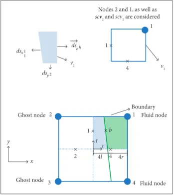
Ghost Sub-Control Volume Type II

In Fig. 7 an element with 2 fluid nodes and two ghost nodes is shown. As mentioned in the section “Sub-Control Volumes and Node Types”, SCVs 1 and 4 are considered ordinary SCVs, and SCVs 2 and 3 are ghost SCVs type II.

Since it is important to remain in the IBM general framework, any point within the flow field (i.e. inside the boundary) and its SCV are considered ordinary. Here Eq. 3 is applied to the whole area of SCV 1, i.e. the area between SS1, SS4, and node 1. Conservation laws for an ordinary SCV were introduced by Eqs. 9-11 in section ghost SCV type I. The actual area within the flow field is the dotted area between SSb, SS4, and node 1 which is shown by grey area in Fig. 6. This area is assigned to ghost node 2 and is called ghost SCV 2. Conservation laws (Eq. 3) are written for this ghost SCV, and boundary condition is applied in these equations. In the present study, boundary condition is applied via ghost SCVs, and not necessarily via the SCVs containing the boundary. Combination of conservation laws for ordinary SCV 1 and ghost SCV 2 will result in the conservation of conserved quantities for the dotted area in SCV 1, which is actually within the flow filed. Implementation of Eq. 3 on ghost SCVs is explained next. Mass conservation equation for the grey area is written as:

dsx

ds_y2 1

1

ds

v2 _v

1 b h

Ghost node 2

4r

4l y

x

1 1

3 4

Ghost node

Fluid node

1 ×

× 4 ×

2

Fluid node Boundary

×

s t

× b 1 ×

× 4

Nodes 2 and 1, as well as scν₂ and scν₁ are considered

Figure 7. Ghost SCV type II (SCV 1 and SCV 2 are considered); the grey area is ghost-SCV type II assigned to node 2; the dotted area is the difference area between complete SCV 1 area and the grey area which contains l uid; 4r is the right part of sub-surface 4; 4l is the left part of sub-surface 4 along the grey area; SSb is the boundary portion in SCV 1; v2 is volume of the grey area; v₁ is complete volume of SCV 1; ds_bh is normal surface vector of boundary in SCV 1 in the direction outward from the grey area; ds_bd is the normal surface vector on SSb in the direction outward from the dotted area; dsx1

1 is normal surface vector of sub-surface 1; ds_y1

4l is normal surface vector related to the left part of sub-surface 4; 1,2,3, and 4 points indicated with cross symbol are ip.

where: →ds_bh is the normal surface vector on SSb. As shown in Fig. 6 surface 4 is divided into 2 parts where the let side is denoted by 4l and the right side denoted by 4r. Mass conservation equations of SCV 1 and SCV 2 are written in the system of equations, and solved simultaneously. In order to obtain the i nal solution of this method, the 2 following equations are combined:

⁄

̂ ⃗⃗⃗⃗

̂ ̂ ̂ ⁄

ρ ̂⃗⃗⃗⃗ ⃗⃗⃗⃗⃗⃗

| ,

|

� ̂⃗⃗⃗⃗ ⃗⃗⃗⃗

|

� ̂⃗⃗⃗⃗ ⃗⃗⃗⃗

(� ̂⃗⃗⃗⃗ ⃗⃗⃗⃗ )

|

⁄

̂ ⃗⃗⃗⃗

̂ ̂ ̂ ⁄

ρ ̂⃗⃗⃗⃗ ⃗⃗⃗⃗⃗⃗

|

| ,

|

� ̂⃗⃗⃗⃗ ⃗⃗⃗⃗

|

� ̂⃗⃗⃗⃗ ⃗⃗⃗⃗

(� ̂⃗⃗⃗⃗ ⃗⃗⃗⃗ )

|

(16)

(17)

where →ds_bd is the normal surface vector on SSb and is equal to –→ds_bh.

Equation 17 is in fact the mass conservation equation for the dotted area with the actual SCV related to node 1. Depending on the boundary condition of the problem, appropriate constraints can be forced in Eq. 16. For instance, if boundary b is solid, then (→pq ˆ _b . →ds_bh) = 0.

Similar procedure is applied for momentum conservation equations. The x-momentum conservation equation for the grey area in Fig. 6 is written as follows: