Frank M White, 5 Ed.

(1)

(2)

McGraw-Hill Series in Mechanical Engineering CONSULTING EDITORS

Jack P. Holman,Southern Methodist University John Lloyd,Michigan State University Anderson

Computational Fluid Dynamics: The Basics with Applications Anderson

Modern Compressible Flow: With Historical Perspective Arora

Introduction to Optimum Design Borman and Ragland

Combustion Engineering Burton

Introduction to Dynamic Systems Analysis Culp

Principles of Energy Conversion Dieter

Engineering Design: A Materials & Processing Approach Doebelin

Engineering Experimentation: Planning, Execution, Reporting Driels

Linear Control Systems Engineering Edwards and McKee

Fundamentals of Mechanical Component Design Gebhart

Heat Conduction and Mass Diffusion Gibson

Principles of Composite Material Mechanics Hamrock

Fundamentals of Fluid Film Lubrication Heywood

Internal Combustion Engine Fundamentals Hinze

Turbulence

Histand and Alciatore

Introduction to Mechatronics and Measurement Systems Holman

Experimental Methods for Engineers Howell and Buckius

Fundamentals of Engineering Thermodynamics Jaluria

Design and Optimization of Thermal Systems Juvinall

Engineering Considerations of Stress, Strain, and Strength Kays and Crawford

Convective Heat and Mass Transfer Kelly

Fundamentals of Mechanical Vibrations

Kimbrell

Kinematics Analysis and Synthesis

Kreider and Rabl

Heating and Cooling of Buildings Martin

Kinematics and Dynamics of Machines Mattingly

Elements of Gas Turbine Propulsion Modest

Radiative Heat Transfer Norton

Design of Machinery

Oosthuizen and Carscallen Compressible Fluid Flow Oosthuizen and Naylor

Introduction to Convective Heat Transfer Analysis

Phelan

Fundamentals of Mechanical Design Reddy

An Introduction to Finite Element Method Rosenberg and Karnopp

Introduction to Physical Systems Dynamics

Schlichting

Boundary-Layer Theory Shames

Mechanics of Fluids

Shigley

Kinematic Analysis of Mechanisms Shigley and Mischke

Mechanical Engineering Design Shigley and Uicker

Theory of Machines and Mechanisms

Stiffler

Design with Microprocessors for Mechanical Engineers Stoecker and Jones

Refrigeration and Air Conditioning

Turns

An Introduction to Combustion: Concepts and Applications Ullman

The Mechanical Design Process Wark

Advanced Thermodynamics for Engineers Wark and Richards

Thermodynamics White

Viscous Fluid Flow

Zeid

(3)

Fluid Mechanics

Fourth Edition

Frank M. White

University of Rhode Island

Boston Burr Ridge, IL Dubuque, IA Madison, WI New York San Francisco St. Louis Bangkok Bogotá Caracas Lisbon London Madrid

(4)

About the Author

Frank M. Whiteis Professor of Mechanical and Ocean Engineering at the University of Rhode Island. He studied at Georgia Tech and M.I.T. In 1966 he helped found, at URI, the first department of ocean engineering in the country. Known primarily as a teacher and writer, he has received eight teaching awards and has written four text-books on fluid mechanics and heat transfer.

During 1979–1990 he was editor-in-chief of the ASME Journal of Fluids Engi-neering and then served from 1991 to 1997 as chairman of the ASME Board of Edi-tors and of the Publications Committee. He is a Fellow of ASME and in 1991 received the ASME Fluids Engineering Award. He lives with his wife, Jeanne, in Narragansett, Rhode Island.

(5)

(6)

General Approach

xi

Preface

The fourth edition of this textbook sees some additions and deletions but no philo-sophical change. The basic outline of eleven chapters and five appendices remains the same. The triad of integral, differential, and experimental approaches is retained and is approached in that order of presentation. The book is intended for an undergraduate course in fluid mechanics, and there is plenty of material for a full year of instruction. The author covers the first six chapters and part of Chapter 7 in the introductory se-mester. The more specialized and applied topics from Chapters 7 to 11 are then cov-ered at our university in a second semester. The informal, student-oriented style is re-tained and, if it succeeds, has the flavor of an interactive lecture by the author.

Approximately 30 percent of the problem exercises, and some fully worked examples, have been changed or are new. The total number of problem exercises has increased to more than 1500 in this fourth edition. The focus of the new problems is on practi-cal and realistic fluids engineering experiences. Problems are grouped according to topic, and some are labeled either with an asterisk (especially challenging) or a com-puter-disk icon (where computer solution is recommended). A number of new pho-tographs and figures have been added, especially to illustrate new design applications and new instruments.

Professor John Cimbala, of Pennsylvania State University, contributed many of the new problems. He had the great idea of setting comprehensive problems at the end of each chapter, covering a broad range of concepts, often from several different chap-ters. These comprehensive problems grow and recur throughout the book as new con-cepts arise. Six more open-ended design projects have been added, making 15 projects in all. The projects allow the student to set sizes and parameters and achieve good de-sign with more than one approach.

An entirely new addition is a set of 95 multiple-choice problems suitable for prepar-ing for the Fundamentals of Engineerprepar-ing (FE) Examination. These FE problems come at the end of Chapters 1 to 10. Meant as a realistic practice for the actual FE Exam, they are engineering problems with five suggested answers, all of them plausible, but only one of them correct.

(7)

Content Changes

New to this book, and to any fluid mechanics textbook, is a special appendix, Ap-pendix E, Introduction to the Engineering Equation Solver (EES), which is keyed to many examples and problems throughout the book. The author finds EES to be an ex-tremely attractive tool for applied engineering problems. Not only does it solve arbi-trarily complex systems of equations, written in any order or form, but also it has built-in property evaluations (density, viscosity, enthalpy, entropy, etc.), lbuilt-inear and nonlbuilt-inear regression, and easily formatted parameter studies and publication-quality plotting. The author is indebted to Professors Sanford Klein and William Beckman, of the Univer-sity of Wisconsin, for invaluable and continuous help in preparing this EES material. The book is now available with or without an EES problems disk. The EES engine is available to adopters of the text with the problems disk.

Another welcome addition, especially for students, is Answers to Selected Prob-lems. Over 600 answers are provided, or about 43 percent of all the regular problem assignments. Thus a compromise is struck between sometimes having a specific nu-merical goal and sometimes directly applying yourself and hoping for the best result.

There are revisions in every chapter. Chapter 1—which is purely introductory and could be assigned as reading—has been toned down from earlier editions. For ex-ample, the discussion of the fluid acceleration vector has been moved entirely to Chap-ter 4. Four brief new sections have been added: (1) the uncertainty of engineering data, (2) the use of EES, (3) the FE Examination, and (4) recommended problem-solving techniques.

Chapter 2 has an improved discussion of the stability of floating bodies, with a fully derived formula for computing the metacentric height. Coverage is confined to static fluids and rigid-body motions. An improved section on pressure measurement discusses modern microsensors, such as the fused-quartz bourdon tube, micromachined silicon capacitive and piezoelectric sensors, and tiny (2 mm long) silicon resonant-frequency devices.

Chapter 3 tightens up the energy equation discussion and retains the plan that Bernoulli’s equation comes last, after control-volume mass, linear momentum, angu-lar momentum, and energy studies. Although some texts begin with an entire chapter on the Bernoulli equation, this author tries to stress that it is a dangerously restricted relation which is often misused by both students and graduate engineers.

In Chapter 4 a few inviscid and viscous flow examples have been added to the ba-sic partial differential equations of fluid mechanics. More extensive discussion con-tinues in Chapter 8.

(8)

Supplements

EES Software

Chapter 8 picks up from the sample plane potential flows of Section 4.10 and plunges right into inviscid-flow analysis, especially aerodynamics. The discussion of numeri-cal methods, or computational fluid dynamics (CFD), both inviscid and viscous, steady and unsteady, has been greatly expanded. Chapter 9, with its myriad complex algebraic equations, illustrates the type of examples and problem assignments which can be solved more easily using EES. A new section has been added about the suborbital X-33 and VentureStar vehicles.

In the discussion of open-channel flow, Chapter 10, we have further attempted to make the material more attractive to civil engineers by adding real-world comprehen-sive problems and design projects from the author’s experience with hydropower proj-ects. More emphasis is placed on the use of friction factors rather than on the Man-ning roughness parameter. Chapter 11, on turbomachinery, has added new material on compressors and the delivery of gases. Some additional fluid properties and formulas have been included in the appendices, which are otherwise much the same.

The all new Instructor’s Resource CD contains a PowerPoint presentation of key text figures as well as additional helpful teaching tools. The list of films and videos, for-merly App. C, is now omitted and relegated to the Instructor’s Resource CD.

The Solutions Manual provides complete and detailed solutions, including prob-lem statements and artwork, to the end-of-chapter probprob-lems. It may be photocopied for posting or preparing transparencies for the classroom.

The Engineering Equation Solver (EES) was developed by Sandy Klein and Bill Beck-man, both of the University of Wisconsin—Madison. A combination of equation-solving capability and engineering property data makes EES an extremely powerful tool for your students. EES (pronounced “ease”) enables students to solve problems, especially design problems, and to ask “what if” questions. EES can do optimization, parametric analysis, linear and nonlinear regression, and provide publication-quality plotting capability. Sim-ple to master, this software allows you to enter equations in any form and in any order. It automatically rearranges the equations to solve them in the most efficient manner.

EES is particularly useful for fluid mechanics problems since much of the property data needed for solving problems in these areas are provided in the program. Air ta-bles are built-in, as are psychometric functions and Joint Army Navy Air Force (JANAF) table data for many common gases. Transport properties are also provided for all sub-stances. EES allows the user to enter property data or functional relationships written in Pascal, C, C⫹⫹, or Fortran. The EES engine is available free to qualified adopters via a password-protected website, to those who adopt the text with the problems disk. The program is updated every semester.

The EES software problems disk provides examples of typical problems in this text. Problems solved are denoted in the text with a disk symbol. Each fully documented solution is actually an EES program that is run using the EES engine. Each program provides detailed comments and on-line help. These programs illustrate the use of EES and help the student master the important concepts without the calculational burden that has been previously required.

(9)

Acknowledgments

So many people have helped me, in addition to Professors John Cimbala, Sanford Klein, and William Beckman, that I cannot remember or list them all. I would like to express my appreciation to many reviewers and correspondents who gave detailed suggestions and materials: Osama Ibrahim, University of Rhode Island; Richard Lessmann, Uni-versity of Rhode Island; William Palm, UniUni-versity of Rhode Island; Deborah Pence, University of Rhode Island; Stuart Tison, National Institute of Standards and Technol-ogy; Paul Lupke, Druck Inc.; Ray Worden, Russka, Inc.; Amy Flanagan, Russka, Inc.; Søren Thalund, Greenland Tourism a/s; Eric Bjerregaard, Greenland Tourism a/s; Mar-tin Girard, DH Instruments, Inc.; Michael Norton, Nielsen-Kellerman Co.; Lisa Colomb, Johnson-Yokogawa Corp.; K. Eisele, Sulzer Innotec, Inc.; Z. Zhang, Sultzer Innotec, Inc.; Helen Reed, Arizona State University; F. Abdel Azim El-Sayed, Zagazig University; Georges Aigret, Chimay, Belgium; X. He, Drexel University; Robert Lo-erke, Colorado State University; Tim Wei, Rutgers University; Tom Conlisk, Ohio State University; David Nelson, Michigan Technological University; Robert Granger, U.S. Naval Academy; Larry Pochop, University of Wyoming; Robert Kirchhoff, University of Massachusetts; Steven Vogel, Duke University; Capt. Jason Durfee, U.S. Military Academy; Capt. Mark Wilson, U.S. Military Academy; Sheldon Green, University of British Columbia; Robert Martinuzzi, University of Western Ontario; Joel Ferziger, Stanford University; Kishan Shah, Stanford University; Jack Hoyt, San Diego State University; Charles Merkle, Pennsylvania State University; Ram Balachandar, Univer-sity of Saskatchewan; Vincent Chu, McGill UniverUniver-sity; and David Bogard, UniverUniver-sity of Texas at Austin.

(10)

Preface xi Chapter 1

Introduction 3

1.1 Preliminary Remarks 3 1.2 The Concept of a Fluid 4 1.3 The Fluid as a Continuum 6 1.4 Dimensions and Units 7

1.5 Properties of the Velocity Field 14 1.6 Thermodynamic Properties of a Fluid 16 1.7 Viscosity and Other Secondary Properties 22 1.8 Basic Flow-Analysis Techniques 35 1.9 Flow Patterns: Streamlines, Streaklines, and

Pathlines 37

1.10 The Engineering Equation Solver 41 1.11 Uncertainty of Experimental Data 42

1.12 The Fundamentals of Engineering (FE) Examination 43 1.13 Problem-Solving Techniques 44

1.14 History and Scope of Fluid Mechanics 44 Problems 46

Fundamentals of Engineering Exam Problems 53 Comprehensive Problems 54

References 55

Chapter 2

Pressure Distribution in a Fluid 59

2.1 Pressure and Pressure Gradient 59 2.2 Equilibrium of a Fluid Element 61 2.3 Hydrostatic Pressure Distributions 63 2.4 Application to Manometry 70

2.5 Hydrostatic Forces on Plane Surfaces 74

vii

hurricanes are strongly affected by the Coriolis acceleration due to the rotation of the earth, which causes them to swirl counterclockwise in the Northern Hemisphere. The physical properties and boundary conditions which govern such flows are discussed in the present chapter. (Courtesy of NASA/Color-Pic Inc./E.R. Degginger/Color-Pic Inc.)

(14)

1.1 Preliminary Remarks

Fluid mechanics is the study of fluids either in motion (fluid dynamics) or at rest (fluid

statics) and the subsequent effects of the fluid upon the boundaries, which may be ei-ther solid surfaces or interfaces with oei-ther fluids. Both gases and liquids are classified as fluids, and the number of fluids engineering applications is enormous: breathing, blood flow, swimming, pumps, fans, turbines, airplanes, ships, rivers, windmills, pipes, missiles, icebergs, engines, filters, jets, and sprinklers, to name a few. When you think about it, almost everything on this planet either is a fluid or moves within or near a fluid.

The essence of the subject of fluid flow is a judicious compromise between theory and experiment. Since fluid flow is a branch of mechanics, it satisfies a set of well-documented basic laws, and thus a great deal of theoretical treatment is available. How-ever, the theory is often frustrating, because it applies mainly to idealized situations which may be invalid in practical problems. The two chief obstacles to a workable the-ory are geometry and viscosity. The basic equations of fluid motion (Chap. 4) are too difficult to enable the analyst to attack arbitrary geometric configurations. Thus most textbooks concentrate on flat plates, circular pipes, and other easy geometries. It is pos-sible to apply numerical computer techniques to complex geometries, and specialized textbooks are now available to explain the new computational fluid dynamics (CFD) approximations and methods [1, 2, 29].1This book will present many theoretical re-sults while keeping their limitations in mind.

The second obstacle to a workable theory is the action of viscosity, which can be neglected only in certain idealized flows (Chap. 8). First, viscosity increases the diffi-culty of the basic equations, although the boundary-layer approximation found by Lud-wig Prandtl in 1904 (Chap. 7) has greatly simplified viscous-flow analyses. Second, viscosity has a destabilizing effect on all fluids, giving rise, at frustratingly small ve-locities, to a disorderly, random phenomenon called turbulence. The theory of turbu-lent flow is crude and heavily backed up by experiment (Chap. 6), yet it can be quite serviceable as an engineering estimate. Textbooks now present digital-computer tech-niques for turbulent-flow analysis [32], but they are based strictly upon empirical as-sumptions regarding the time mean of the turbulent stress field.

Chapter 1 Introduction

(15)

1.2 The Concept of a Fluid

Thus there is theory available for fluid-flow problems, but in all cases it should be backed up by experiment. Often the experimental data provide the main source of in-formation about specific flows, such as the drag and lift of immersed bodies (Chap. 7). Fortunately, fluid mechanics is a highly visual subject, with good instrumentation [4, 5, 35], and the use of dimensional analysis and modeling concepts (Chap. 5) is wide-spread. Thus experimentation provides a natural and easy complement to the theory. You should keep in mind that theory and experiment should go hand in hand in all studies of fluid mechanics.

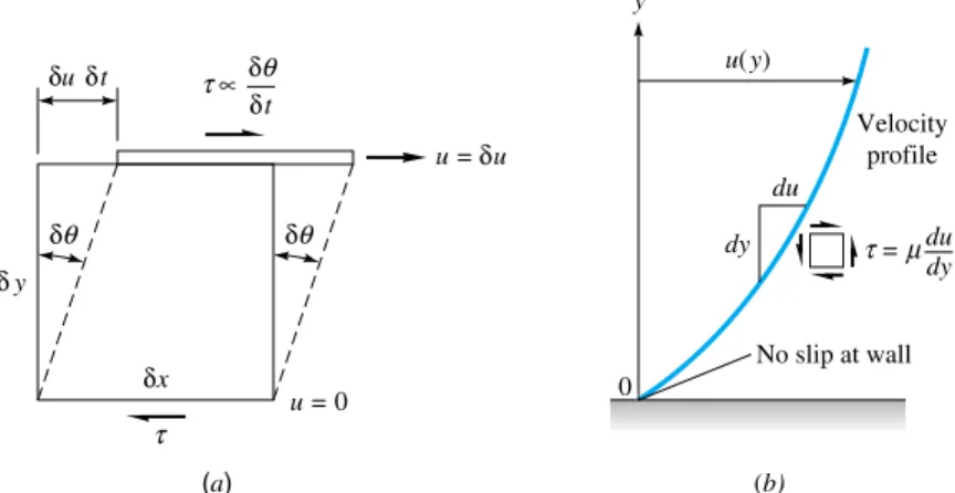
From the point of view of fluid mechanics, all matter consists of only two states, fluid and solid. The difference between the two is perfectly obvious to the layperson, and it is an interesting exercise to ask a layperson to put this difference into words. The tech-nical distinction lies with the reaction of the two to an applied shear or tangential stress.

A solid can resist a shear stress by a static deformation; a fluid cannot. Any shear stress applied to a fluid, no matter how small, will result in motion of that fluid. The fluid moves and deforms continuously as long as the shear stress is applied. As a corol-lary, we can say that a fluid at rest must be in a state of zero shear stress, a state of-ten called the hydrostatic stress condition in structural analysis. In this condition, Mohr’s circle for stress reduces to a point, and there is no shear stress on any plane cut through the element under stress.

Given the definition of a fluid above, every layperson also knows that there are two classes of fluids,liquidsand gases. Again the distinction is a technical one concerning the effect of cohesive forces. A liquid, being composed of relatively close-packed mol-ecules with strong cohesive forces, tends to retain its volume and will form a free sur-face in a gravitational field if unconfined from above. Free-sursur-face flows are domi-nated by gravitational effects and are studied in Chaps. 5 and 10. Since gas molecules are widely spaced with negligible cohesive forces, a gas is free to expand until it en-counters confining walls. A gas has no definite volume, and when left to itself with-out confinement, a gas forms an atmosphere which is essentially hydrostatic. The hy-drostatic behavior of liquids and gases is taken up in Chap. 2. Gases cannot form a free surface, and thus gas flows are rarely concerned with gravitational effects other than buoyancy.

Figure 1.1 illustrates a solid block resting on a rigid plane and stressed by its own weight. The solid sags into a static deflection, shown as a highly exaggerated dashed line, resisting shear without flow. A free-body diagram of element Aon the side of the block shows that there is shear in the block along a plane cut at an angle through A. Since the block sides are unsupported, element Ahas zero stress on the left and right sides and compression stress pon the top and bottom. Mohr’s circle does not reduce to a point, and there is nonzero shear stress in the block.

(16)

configura-tion, pouring out over the lip if necessary. Meanwhile, the gas is unrestrained and ex-pands out of the container, filling all available space. Element Ain the gas is also hy-drostatic and exerts a compression stress pon the walls.

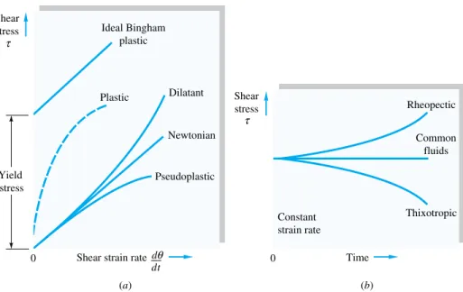
In the above discussion, clear decisions could be made about solids, liquids, and gases. Most engineering fluid-mechanics problems deal with these clear cases, i.e., the common liquids, such as water, oil, mercury, gasoline, and alcohol, and the common gases, such as air, helium, hydrogen, and steam, in their common temperature and pres-sure ranges. There are many borderline cases, however, of which you should be aware. Some apparently “solid” substances such as asphalt and lead resist shear stress for short periods but actually deform slowly and exhibit definite fluid behavior over long peri-ods. Other substances, notably colloid and slurry mixtures, resist small shear stresses but “yield” at large stress and begin to flow as fluids do. Specialized textbooks are de-voted to this study of more general deformation and flow, a field called rheology[6]. Also, liquids and gases can coexist in two-phase mixtures, such as steam-water mix-tures or water with entrapped air bubbles. Specialized textbooks present the analysis 1.2 The Concept of a Fluid 5

Static deflection

Free surface

Hydrostatic condition Liquid Solid

A A A

(a) (c)

(b) (d)

0 0

A A

Gas

(1)

– p – p

p p

p

= 0

τ θ θ

θ

2

1

– = p – = p

σ σ

1

τ σ

τ

σ

τ

σ Fig. 1.1A solid at rest can resist

(17)

1.3 The Fluid as a Continuum

of such two-phase flows[7]. Finally, there are situations where the distinction between a liquid and a gas blurs. This is the case at temperatures and pressures above the so-called critical pointof a substance, where only a single phase exists, primarily resem-bling a gas. As pressure increases far above the critical point, the gaslike substance be-comes so dense that there is some resemblance to a liquid and the usual thermodynamic approximations like the perfect-gas law become inaccurate. The critical temperature and pressure of water are Tc647 K and pc219 atm,2so that typical problems in-volving water and steam are below the critical point. Air, being a mixture of gases, has no distinct critical point, but its principal component, nitrogen, hasTc126 K and

pc34 atm. Thus typical problems involving air are in the range of high temperature and low pressure where air is distinctly and definitely a gas. This text will be concerned solely with clearly identifiable liquids and gases, and the borderline cases discussed above will be beyond our scope.

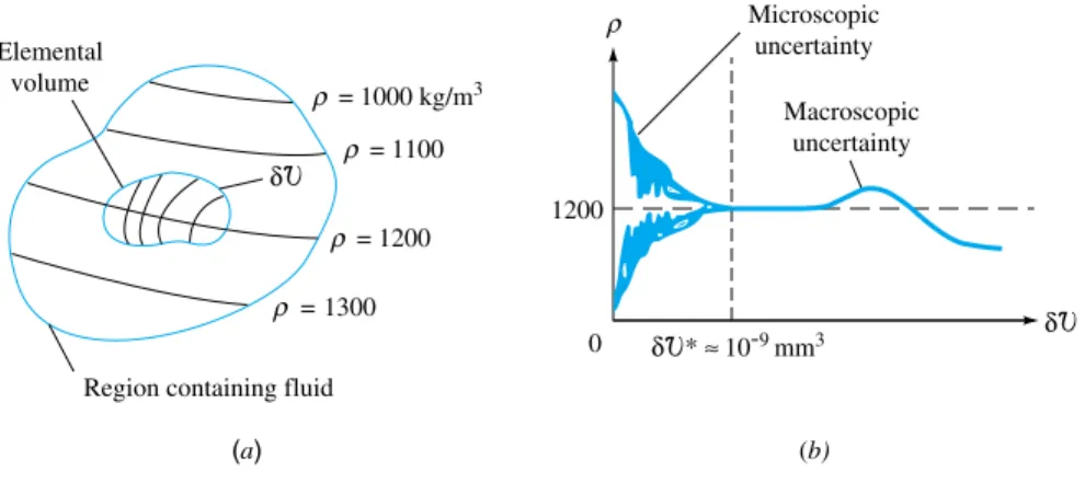
We have already used technical terms such as fluid pressureand densitywithout a rig-orous discussion of their definition. As far as we know, fluids are aggregations of ecules, widely spaced for a gas, closely spaced for a liquid. The distance between mol-ecules is very large compared with the molecular diameter. The molmol-ecules are not fixed in a lattice but move about freely relative to each other. Thus fluid density, or mass per unit volume, has no precise meaning because the number of molecules occupying a given volume continually changes. This effect becomes unimportant if the unit volume is large compared with, say, the cube of the molecular spacing, when the number of molecules within the volume will remain nearly constant in spite of the enormous in-terchange of particles across the boundaries. If, however, the chosen unit volume is too large, there could be a noticeable variation in the bulk aggregation of the particles. This situation is illustrated in Fig. 1.2, where the “density” as calculated from molecular mass mwithin a given volume ᐂ_{is plotted versus the size of the unit volume. There} is a limiting volume ᐂ_{* below which molecular variations may be important and}

Microscopic uncertainty

Macroscopic uncertainty

0 1200

δ

δ * ≈ 10-9 _mm3

Elemental volume

Region containing fluid

= 1000 kg/m3

= 1100

= 1200

= 1300

(a) (b)

ρ ρ

ρ

ρ ρ

δ Fig. 1.2The limit definition of

con-tinuum fluid density: (a) an ele-mental volume in a fluid region of variable continuum density; (b) cal-culated density versus size of the elemental volume.

2

(18)

1.4 Dimensions and Units

above which aggregate variations may be important. The density of a fluid is best defined as

lim

ᐂ→ᐂ*

ᐂ

m

(1.1)

The limiting volume ᐂ_{* is about 10}9_mm3_{for all liquids and for gases at atmospheric}

pressure. For example, 109_mm3_{of air at standard conditions contains approximately}

3 107_{molecules, which is sufficient to define a nearly constant density according to}

Eq. (1.1). Most engineering problems are concerned with physical dimensions much larger than this limiting volume, so that density is essentially a point function and fluid proper-ties can be thought of as varying continually in space, as sketched in Fig. 1.2a. Such a fluid is called a continuum,which simply means that its variation in properties is so smooth that the differential calculus can be used to analyze the substance. We shall assume that continuum calculus is valid for all the analyses in this book. Again there are borderline cases for gases at such low pressures that molecular spacing and mean free path3_are

com-parable to, or larger than, the physical size of the system. This requires that the contin-uum approximation be dropped in favor of a molecular theory of rarefied-gas flow [8]. In principle, all fluid-mechanics problems can be attacked from the molecular viewpoint, but no such attempt will be made here. Note that the use of continuum calculus does not pre-clude the possibility of discontinuous jumps in fluid properties across a free surface or fluid interface or across a shock wave in a compressible fluid (Chap. 9). Our calculus in Chap. 4 must be flexible enough to handle discontinuous boundary conditions.

A dimensionis the measure by which a physical variable is expressed quantitatively. A unitis a particular way of attaching a number to the quantitative dimension. Thus length is a dimension associated with such variables as distance, displacement, width, deflection, and height, while centimeters and inches are both numerical units for ex-pressing length. Dimension is a powerful concept about which a splendid tool called

dimensional analysishas been developed (Chap. 5), while units are the nitty-gritty, the number which the customer wants as the final answer.

Systems of units have always varied widely from country to country, even after in-ternational agreements have been reached. Engineers need numbers and therefore unit systems, and the numbers must be accurate because the safety of the public is at stake. You cannot design and build a piping system whose diameter is Dand whose length is L. And U.S. engineers have persisted too long in clinging to British systems of units. There is too much margin for error in most British systems, and many an engineering student has flunked a test because of a missing or improper conversion factor of 12 or 144 or 32.2 or 60 or 1.8. Practicing engineers can make the same errors. The writer is aware from personal experience of a serious preliminary error in the design of an air-craft due to a missing factor of 32.2 to convert pounds of mass to slugs.

In 1872 an international meeting in France proposed a treaty called the Metric Con-vention, which was signed in 1875 by 17 countries including the United States. It was an improvement over British systems because its use of base 10 is the foundation of our number system, learned from childhood by all. Problems still remained because 1.4 Dimensions and Units 7

(19)

even the metric countries differed in their use of kiloponds instead of dynes or new-tons, kilograms instead of grams, or calories instead of joules. To standardize the met-ric system, a General Conference of Weights and Measures attended in 1960 by 40 countries proposed the International System of Units(SI). We are now undergoing a painful period of transition to SI, an adjustment which may take many more years to complete. The professional societies have led the way. Since July 1, 1974, SI units have been required by all papers published by the American Society of Mechanical Engi-neers, which prepared a useful booklet explaining the SI [9]. The present text will use SI units together with British gravitational (BG) units.

In fluid mechanics there are only four primary dimensions from which all other dimen-sions can be derived: mass, length, time, and temperature.4_{These dimensions and their units}

in both systems are given in Table 1.1. Note that the kelvin unit uses no degree symbol. The braces around a symbol like {M} mean “the dimension” of mass. All other variables in fluid mechanics can be expressed in terms of {M}, {L}, {T}, and {}. For example, ac-celeration has the dimensions {LT2}. The most crucial of these secondary dimensions is force, which is directly related to mass, length, and time by Newton’s second law

Fma (1.2)

From this we see that, dimensionally, {F}{MLT2}. A constant of proportionality is avoided by defining the force unit exactly in terms of the primary units. Thus we define the newton and the pound of force

1 newton of force1 N⬅1 kgm/s2

(1.3) 1 pound of force1 lbf⬅1 slugft/s2_{4.4482 N}

In this book the abbreviation lbfis used for pound-force and lbfor pound-mass. If in-stead one adopts other force units such as the dyne or the poundal or kilopond or adopts other mass units such as the gram or pound-mass, a constant of proportionality called

gcmust be included in Eq. (1.2). We shall not use gcin this book since it is not nec-essary in the SI and BG systems.

A list of some important secondary variables in fluid mechanics, with dimensions derived as combinations of the four primary dimensions, is given in Table 1.2. A more complete list of conversion factors is given in App. C.

4_{If electromagnetic effects are important, a fifth primary dimension must be included, electric current}

{I}, whose SI unit is the ampere (A).

Primary dimension SI unit BG unit Conversion factor

Mass {M} Kilogram (kg) Slug 1 slug14.5939 kg

Length {L} Meter (m) Foot (ft) 1 ft0.3048 m

Time {T} Second (s) Second (s) 1 s1 s

Temperature {} Kelvin (K) Rankine (°R) 1 K1.8°R

Table 1.1Primary Dimensions in SI and BG Systems

(20)

Part (a)

Part (b)

Part (c)

EXAMPLE 1.1

A body weighs 1000 lbf when exposed to a standard earth gravity g32.174 ft/s2_{. (}

a) What is its mass in kg? (b) What will the weight of this body be in N if it is exposed to the moon’s stan-dard acceleration gmoon1.62 m/s2? (c) How fast will the body accelerate if a net force of 400

lbf is applied to it on the moon or on the earth?

Solution

Equation (1.2) holds with Fweight and agearth:

FWmg1000 lbf(mslugs)(32.174 ft/s2₎

or

m

3 1 2 0 .1

0 7 0

4 (31.08 slugs)(14.5939 kg/slug)453.6 kg Ans. (a) The change from 31.08 slugs to 453.6 kg illustrates the proper use of the conversion factor 14.5939 kg/slug.

The mass of the body remains 453.6 kg regardless of its location. Equation (1.2) applies with a new value of aand hence a new force

FWmoonmgmoon(453.6 kg)(1.62 m/s 2

)735 N Ans. (b)

This problem does not involve weight or gravity or position and is simply a direct application of Newton’s law with an unbalanced force:

F400 lbfma(31.08 slugs)(aft/s2₎

or

a

3 4 1 0 .0

0

8 12.43 ft/s

2

3.79 m/s2 Ans. (c)

This acceleration would be the same on the moon or earth or anywhere.

1.4 Dimensions and Units 9

Secondary dimension SI unit BG unit Conversion factor

Area {L2} m2 _ft2 _{1 m}2_{10.764 ft}2

Volume {L3} m3 _ft3 _{1 m}3_{35.315 ft}3

Velocity {LT1} m/s ft/s 1 ft/s0.3048 m/s

Acceleration {LT2} m/s2 _ft/s2 _{1 ft/s}2_{0.3048 m/s}2

Pressure or stress

{ML1T2} PaN/m2 _lbf/ft2 _{1 lbf/ft}2_{47.88 Pa}

Angular velocity {T1} s1 _s1 _{1 s}1_{1 s}1

Energy, heat, work

{ML2T2} JNm ftlbf 1 ftlbf1.3558 J

Power {ML2T3} WJ/s ftlbf/s 1 ftlbf/s1.3558 W Density {ML3} kg/m3 _slugs/ft3 _{1 slug/ft}3_{515.4 kg/m}3

Viscosity {ML1T1} kg/(ms) slugs/(fts) 1 slug/(fts)47.88 kg/(ms) Specific heat {L2T21_} _m2_/(s2_K) _ft2_/(s2_°R) _{1 m}2_/(s2_K)_{5.980 ft}2_/(s2_°R) Table 1.2Secondary Dimensions in

(21)

Part (a)

Part (b)

Many data in the literature are reported in inconvenient or arcane units suitable only to some industry or specialty or country. The engineer should convert these data to the SI or BG system before using them. This requires the systematic application of con-version factors, as in the following example.

EXAMPLE 1.2

An early viscosity unit in the cgs system is the poise (abbreviated P), or g/(cms), named after J. L. M. Poiseuille, a French physician who performed pioneering experiments in 1840 on wa-ter flow in pipes. The viscosity of wawa-ter (fresh or salt) at 293.16 K20°C is approximately

0.01 P. Express this value in (a) SI and (b) BG units.

Solution

[0.01 g/(cms)]

10 1 0

k 0

g g

(100 cm/m)0.001 kg/(ms) Ans. (a)

[0.001 kg/(ms)]

14 1 .5

sl 9

ug kg

(0.3048 m/ft)

2.09 105

slug/(fts) Ans. (b)

Note:Result (b) could have been found directly from (a) by dividing (a) by the viscosity con-version factor 47.88 listed in Table 1.2.

We repeat our advice: Faced with data in unusual units, convert them immediately to either SI or BG units because (1) it is more professional and (2) theoretical equa-tions in fluid mechanics are dimensionally consistentand require no further conversion factors when these two fundamental unit systems are used, as the following example shows.

EXAMPLE 1.3

A useful theoretical equation for computing the relation between pressure, velocity, and altitude in a steady flow of a nearly inviscid, nearly incompressible fluid with negligible heat transfer and shaft work5is the Bernoulli relation,named after Daniel Bernoulli, who published a hy-drodynamics textbook in 1738:

p0p12V2gZ (1)

where p0stagnation pressure

ppressure in moving fluid

Vvelocity density

Zaltitude

ggravitational acceleration

(22)

Part (a)

Part (b)

Part (c)

(a) Show that Eq. (1) satisfies the principle of dimensional homogeneity, which states that all additive terms in a physical equation must have the same dimensions. (b) Show that consistent units result without additional conversion factors in SI units. (c) Repeat (b) for BG units.

Solution

We can express Eq. (1) dimensionally, using braces by entering the dimensions of each term from Table 1.2:

{ML1T2}{ML1T2}{ML3}{L2T2}{ML3}{LT2}{L}

{ML1T2} for all terms Ans. (a)

Enter the SI units for each quantity from Table 1.2:

{N/m2}{N/m2}{kg/m3}{m2/s2}{kg/m3}{m/s2}{m}

{N/m2}{kg/(ms2)}

The right-hand side looks bad until we remember from Eq. (1.3) that 1 kg1 Ns2/m. {kg/(ms2_)} {N

{m

s

2

s /

2

m } }

{N/m2_}

Ans. (b)

Thus all terms in Bernoulli’s equation will have units of pascals, or newtons per square meter, when SI units are used. No conversion factors are needed, which is true of all theoretical equa-tions in fluid mechanics.

Introducing BG units for each term, we have

{lbf/ft2_}_{lbf/ft2_}_{slugs/ft3_}{ft2_/s2_}_{slugs/ft3_}{ft/s2_}{ft}

{lbf/ft2_}_{slugs/(ft_s2_)}

But, from Eq. (1.3), 1 slug1 lbfs2_{/ft, so that}

{slugs/(fts2_)} {l

{ b f f t

s s

2

/ } ft}

{lbf/ft2_}

Ans. (c)

All terms have the unit of pounds-force per square foot. No conversion factors are needed in the BG system either.

There is still a tendency in English-speaking countries to use pound-force per square inch as a pressure unit because the numbers are more manageable. For example, stan-dard atmospheric pressure is 14.7 lbf/in2_{2116 lbf/ft}2_{101,300 Pa. The pascal is a}

small unit because the newton is less than 1

4lbf and a square meter is a very large area.

It is felt nevertheless that the pascal will gradually gain universal acceptance; e.g., re-pair manuals for U.S. automobiles now specify pressure measurements in pascals.

Note that not only must all (fluid) mechanics equations be dimensionally homogeneous, one must also use consistent units; that is, each additive term must have the same units. There is no trouble doing this with the SI and BG systems, as in Ex. 1.3, but woe unto 1.4 Dimensions and Units 11

(23)

Homogeneous versus Dimensionally Inconsistent Equations

those who try to mix colloquial English units. For example, in Chap. 9, we often use the assumption of steady adiabatic compressible gas flow:

h1 2V

2_constant

where h is the fluid enthalpy and V2/2 is its kinetic energy. Colloquial thermodynamic tables might list h in units of British thermal units per pound (Btu/lb), whereas V is likely used in ft/s. It is completely erroneous to add Btu/lb to ft2/s2. The proper unit for h in this case is ftlbf/slug, which is identical to ft2/s2. The conversion factor is 1 Btu/lb⬇25,040 ft2/s225,040 ftlbf/slug.

All theoretical equations in mechanics (and in other physical sciences) are dimension-ally homogeneous; i.e., each additive term in the equation has the same dimensions. For example, Bernoulli’s equation (1) in Example 1.3 is dimensionally homogeneous: Each term has the dimensions of pressure or stress of {F/L2}. Another example is the equation from physics for a body falling with negligible air resistance:

SS0V0t12gt 2

where S0is initial position,V0is initial velocity, and gis the acceleration of gravity. Each

term in this relation has dimensions of length {L}. The factor 1₂_{, which arises from} inte-gration, is a pure (dimensionless) number, {1}. The exponent 2 is also dimensionless. However, the reader should be warned that many empirical formulas in the engi-neering literature, arising primarily from correlations of data, are dimensionally in-consistent. Their units cannot be reconciled simply, and some terms may contain hid-den variables. An example is the formula which pipe valve manufacturers cite for liquid volume flow rate Q(m3/s) through a partially open valve:

QCV

冢

S

G

p

冣

1/2

where pis the pressure drop across the valve and SG is the specific gravity of the liquid (the ratio of its density to that of water). The quantity CVis the valve flow

co-efficient, which manufacturers tabulate in their valve brochures. Since SG is dimen-sionless {1}, we see that this formula is totally inconsistent, with one side being a flow rate {L3/T} and the other being the square root of a pressure drop {M1/2/L1/2T}. It fol-lows that CVmust have dimensions, and rather odd ones at that: {L

7/2

/M1/2}. Nor is the resolution of this discrepancy clear, although one hint is that the values of CVin the literature increase nearly as the square of the size of the valve. The presentation of experimental data in homogeneous form is the subject of dimensional analysis(Chap. 5). There we shall learn that a homogeneous form for the valve flow relation is

QCdAopening

冢

p

冣

1/2

(24)

Convenient Prefixes in Powers of 10

Part (a)

Part (b)

Meanwhile, we conclude that dimensionally inconsistent equations, though they abound in engineering practice, are misleading and vague and even dangerous, in the sense that they are often misused outside their range of applicability.

Engineering results often are too small or too large for the common units, with too many zeros one way or the other. For example, to write p114,000,000 Pa is long and awkward. Using the prefix “M” to mean 106, we convert this to a concise p

114 MPa (megapascals). Similarly, t0.000000003 s is a proofreader’s nightmare compared to the equivalent t3 ns (nanoseconds). Such prefixes are common and convenient, in both the SI and BG systems. A complete list is given in Table 1.3.

EXAMPLE 1.4

In 1890 Robert Manning, an Irish engineer, proposed the following empirical formula for the average velocity Vin uniform flow due to gravity down an open channel (BG units):

V 1. n

49

R2/3S1/2 (1)

where Rhydraulic radius of channel (Chaps. 6 and 10)

Schannel slope (tangent of angle that bottom makes with horizontal)

nManning’s roughness factor (Chap. 10)

and nis a constant for a given surface condition for the walls and bottom of the channel. (a) Is Manning’s formula dimensionally consistent? (b) Equation (1) is commonly taken to be valid in BG units with ntaken as dimensionless. Rewrite it in SI form.

Solution

Introduce dimensions for each term. The slope S,being a tangent or ratio, is dimensionless, de-noted by {unity} or {1}. Equation (1) in dimensional form is

冦

T L

冧

冦

1.

n

49

冧

{L2/3}{1}

This formula cannot be consistent unless {1.49/n}{L1/3/T}. If nis dimensionless (and it is never listed with units in textbooks), then the numerical value 1.49 must have units. This can be tragic to an engineer working in a different unit system unless the discrepancy is properly doc-umented. In fact, Manning’s formula, though popular, is inconsistent both dimensionally and physically and does not properly account for channel-roughness effects except in a narrow range of parameters, for water only.

From part (a), the number 1.49 must have dimensions {L1/3/T} and thus in BG units equals 1.49 ft1/3/s. By using the SI conversion factor for length we have

(1.49 ft1/3/s)(0.3048 m/ft)1/31.00 m1/3/s Therefore Manning’s formula in SI becomes

V 1

n

.0

R2/3S1/2 Ans. (b)(2)

1.4 Dimensions and Units 13

Table 1.3Convenient Prefixes for Engineering Units

Multiplicative

factor Prefix Symbol

1012 _tera _T

109 _giga _G

106 _mega _M

103 _kilo _k

102 _hecto _h

10 deka da

101 _deci _d

102 _centi _c

103 _milli _m

106 _micro

109 _nano _n

1012 _pico _p

1015 _femto _f

(25)

1.5 Properties of the

Velocity Field

Eulerian and Lagrangian Desciptions

The Velocity Field

with Rin m and Vin m/s. Actually, we misled you: This is the way Manning, a metric user, first proposed the formula. It was later converted to BG units. Such dimensionally inconsistent formu-las are dangerous and should either be reanalyzed or treated as having very limited application.

In a given flow situation, the determination, by experiment or theory, of the properties of the fluid as a function of position and time is considered to be the solutionto the problem. In almost all cases, the emphasis is on the space-time distribution of the fluid properties. One rarely keeps track of the actual fate of the specific fluid particles.6This treatment of properties as continuum-field functions distinguishes fluid mechanics from solid mechanics, where we are more likely to be interested in the trajectories of indi-vidual particles or systems.

There are two different points of view in analyzing problems in mechanics. The first view, appropriate to fluid mechanics, is concerned with the field of flow and is called the eulerian method of description. In the eulerian method we compute the pressure field p(x,y,z,t) of the flow pattern, not the pressure changes p(t) which a particle ex-periences as it moves through the field.

The second method, which follows an individual particle moving through the flow, is called the lagrangian description. The lagrangian approach, which is more appro-priate to solid mechanics, will not be treated in this book. However, certain numerical analyses of sharply bounded fluid flows, such as the motion of isolated fluid droplets, are very conveniently computed in lagrangian coordinates [1].

Fluid-dynamic measurements are also suited to the eulerian system. For example, when a pressure probe is introduced into a laboratory flow, it is fixed at a specific po-sition (x,y,z). Its output thus contributes to the description of the eulerian pressure field p(x,y,z,t). To simulate a lagrangian measurement, the probe would have to move downstream at the fluid particle speeds; this is sometimes done in oceanographic mea-surements, where flowmeters drift along with the prevailing currents.

The two different descriptions can be contrasted in the analysis of traffic flow along a freeway. A certain length of freeway may be selected for study and called the field of flow. Obviously, as time passes, various cars will enter and leave the field, and the identity of the specific cars within the field will constantly be changing. The traffic en-gineer ignores specific cars and concentrates on their average velocity as a function of time and position within the field, plus the flow rate or number of cars per hour pass-ing a given section of the freeway. This engineer is uspass-ing an eulerian description of the traffic flow. Other investigators, such as the police or social scientists, may be inter-ested in the path or speed or destination of specific cars in the field. By following a specific car as a function of time, they are using a lagrangian description of the flow.

Foremost among the properties of a flow is the velocity field V(x,y,z,t). In fact, de-termining the velocity is often tantamount to solving a flow problem, since other

prop-6_{One example where fluid-particle paths are important is in water-quality analysis of the fate of}

(26)

erties follow directly from the velocity field. Chapter 2 is devoted to the calculation of the pressure field once the velocity field is known. Books on heat transfer (for exam-ple, Ref. 10) are essentially devoted to finding the temperature field from known ve-locity fields.

In general, velocity is a vector function of position and time and thus has three com-ponents u,v, and w, each a scalar field in itself:

V(x,y,z,t)iu(x,y,z,t)jv(x,y,z,t)kw(x,y,z,t) (1.4) The use of u,v, and winstead of the more logical component notation Vx,Vy, and Vz is the result of an almost unbreakable custom in fluid mechanics.

Several other quantities, called kinematic properties,can be derived by mathemati-cally manipulating the velocity field. We list some kinematic properties here and give more details about their use and derivation in later chapters:

1. Displacement vector: r

冕

Vdt (Sec. 1.9)

2. Acceleration: a d

d

V

t

(Sec. 4.1)

3. Volume rate of flow: Q

冕

(Vⴢn)dA (Sec. 3.2)

4. Volume expansion rate:

ᐂ 1 d

d

ᐂ

t

ⴢV (Sec. 4.2)

5. Local angular velocity: 1₂_V _{(Sec. 4.8)}

We will not illustrate any problems regarding these kinematic properties at present. The point of the list is to illustrate the type of vector operations used in fluid mechanics and to make clear the dominance of the velocity field in determining other flow properties.

Note:The fluid acceleration,item 2 above, is not as simple as it looks and actually in-volves four different terms due to the use of the chain rule in calculus (see Sec. 4.1).

EXAMPLE 1.5

Fluid flows through a contracting section of a duct, as in Fig. E1.5. A velocity probe inserted at section (1) measures a steady value u11 m/s, while a similar probe at section (2) records a

steady u23 m/s. Estimate the fluid acceleration, if any, if x10 cm.

Solution

The flow is steady (not time-varying), but fluid particles clearly increase in velocity as they pass from (1) to (2). This is the concept of convective acceleration (Sec. 4.1). We may estimate the acceleration as a velocity change udivided by a time change t x/uavg:

ax⬇

ve t l i o m

c e ity

ch c

a h

n a

g n

e ge

⬇ ⬇40 m/s2 _Ans.

A simple estimate thus indicates that this seemingly innocuous flow is accelerating at 4 times (3.01.0 m/s)(1.03.0 m/s)

2(0.1 m)

u2u1

x/[1

2(u1u2)]

1.5 Properties of the Velocity Field 15

(1)

(2)

u₁ u₂

(27)

1.6 Thermodynamic Properties

of a Fluid

the acceleration of gravity. In the limit as xand tbecome very small, the above estimate re-duces to a partial-derivative expression for convective x-acceleration:

ax,convectivelim

t→0

u t u

u x

In three-dimensional flow (Sec. 4.1) there are nine of these convective terms.

While the velocity field Vis the most important fluid property, it interacts closely with the thermodynamic properties of the fluid. We have already introduced into the dis-cussion the three most common such properties

1. Pressure p

2. Density

3. Temperature T

These three are constant companions of the velocity vector in flow analyses. Four other thermodynamic properties become important when work, heat, and energy balances are treated (Chaps. 3 and 4):

4. Internal energy e

5. Enthalpy hûp/

6. Entropy s

7. Specific heats cpand cv

In addition, friction and heat conduction effects are governed by the two so-called trans-port properties:

8. Coefficient of viscosity

9. Thermal conductivity k

All nine of these quantities are true thermodynamic properties which are determined by the thermodynamic condition or stateof the fluid. For example, for a single-phase substance such as water or oxygen, two basic properties such as pressure and temper-ature are sufficient to fix the value of all the others:

(p,T) hh(p,T) (p,T) (1.5)

and so on for every quantity in the list. Note that the specific volume, so important in thermodynamic analyses, is omitted here in favor of its inverse, the density .

Recall that thermodynamic properties describe the state of a system,i.e., a collec-tion of matter of fixed identity which interacts with its surroundings. In most cases here the system will be a small fluid element, and all properties will be assumed to be continuum properties of the flow field: (x,y,z,t), etc.

(28)

ad-Temperature

Specific Weight Density

justs itself toward equilibrium. We therefore assume that all the thermodynamic prop-erties listed above exist as point functions in a flowing fluid and follow all the laws and state relations of ordinary equilibrium thermodynamics. There are, of course, im-portant nonequilibrium effects such as chemical and nuclear reactions in flowing flu-ids which are not treated in this text.

Pressure is the (compression) stress at a point in a static fluid (Fig. 1.1). Next to ve-locity, the pressure pis the most dynamic variable in fluid mechanics. Differences or

gradientsin pressure often drive a fluid flow, especially in ducts. In low-speed flows, the actual magnitude of the pressure is often not important, unless it drops so low as to cause vapor bubbles to form in a liquid. For convenience, we set many such problem assignments at the level of 1 atm2116 lbf/ft2101,300 Pa. High-speed (compressible) gas flows (Chap. 9), however, are indeed sensitive to the magnitude of pressure.

Temperature T is a measure of the internal energy level of a fluid. It may vary con-siderably during high-speed flow of a gas (Chap. 9). Although engineers often use Cel-sius or Fahrenheit scales for convenience, many applications in this text require ab-solute(Kelvin or Rankine) temperature scales:

°R°F459.69 K°C273.16

If temperature differences are strong,heat transfermay be important [10], but our con-cern here is mainly with dynamic effects. We examine heat-transfer principles briefly in Secs. 4.5 and 9.8.

The density of a fluid, denoted by (lowercase Greek rho), is its mass per unit vol-ume. Density is highly variable in gases and increases nearly proportionally to the pres-sure level. Density in liquids is nearly constant; the density of water (about 1000 kg/m3₎

increases only 1 percent if the pressure is increased by a factor of 220. Thus most liq-uid flows are treated analytically as nearly “incompressible.”

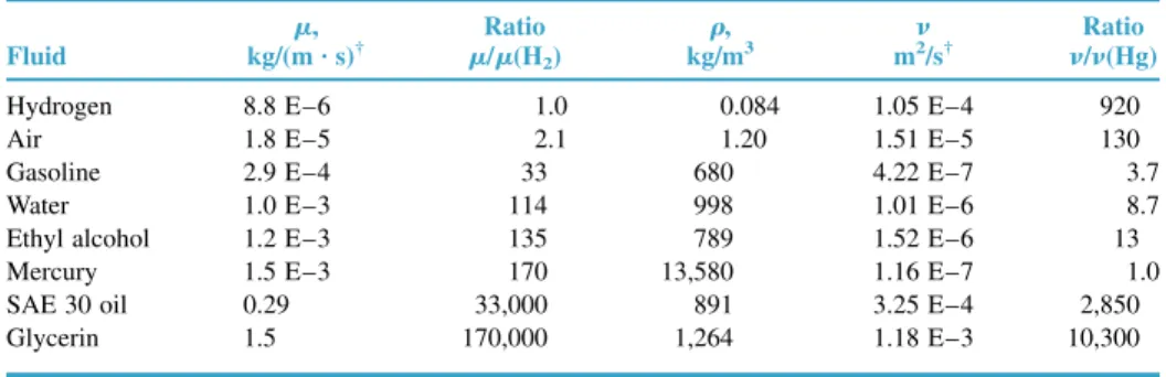
In general, liquids are about three orders of magnitude more dense than gases at at-mospheric pressure. The heaviest common liquid is mercury, and the lightest gas is hy-drogen. Compare their densities at 20°C and 1 atm:

Mercury: 13,580 kg/m3 _Hydrogen: _{0.0838 kg/m}3

They differ by a factor of 162,000! Thus the physical parameters in various liquid and gas flows might vary considerably. The differences are often resolved by the use of di-mensional analysis(Chap. 5). Other fluid densities are listed in Tables A.3 and A.4 (in App. A).

The specific weightof a fluid, denoted by (lowercase Greek gamma), is its weight per unit volume. Just as a mass has a weight Wmg, density and specific weight are simply related by gravity:

g (1.6)

1.6 Thermodynamic Properties of a Fluid 17

(29)

Specific Gravity

Potential and Kinetic Energies

The units of are weight per unit volume, in lbf/ft3or N/m3. In standard earth grav-ity,g32.174 ft/s29.807 m/s2. Thus, e.g., the specific weights of air and water at 20°C and 1 atm are approximately

air(1.205 kg/m3)(9.807 m/s2)11.8 N/m30.0752 lbf/ft3

water(998 kg/m3)(9.807 m/s2)9790 N/m362.4 lbf/ft3

Specific weight is very useful in the hydrostatic-pressure applications of Chap. 2. Spe-cific weights of other fluids are given in Tables A.3 and A.4.

Specific gravity,denoted by SG, is the ratio of a fluid density to a standard reference fluid, water (for liquids), and air (for gases):

SGgas

g

a a

ir s

1.20

5

g

k

as

g/m3

(1.7)

SGliquid

l

w iq

a u

te id

r

99

8

li

k

qu

g

i

/

d

m3

For example, the specific gravity of mercury (Hg) is SGHg13,580/998⬇13.6.

En-gineers find these dimensionless ratios easier to remember than the actual numerical values of density of a variety of fluids.

In thermostatics the only energy in a substance is that stored in a system by molecu-lar activity and molecumolecu-lar bonding forces. This is commonly denoted as internal en-ergy û. A commonly accepted adjustment to this static situation for fluid flow is to add two more energy terms which arise from newtonian mechanics: the potential energy and kinetic energy.

The potential energy equals the work required to move the system of mass mfrom the origin to a position vector rixjykzagainst a gravity field g. Its value is

mgⴢr, or gⴢrper unit mass. The kinetic energy equals the work required to change the speed of the mass from zero to velocity V. Its value is 1

2mV2or 12V2per unit mass.

Then by common convention the total stored energy eper unit mass in fluid mechan-ics is the sum of three terms:

eû1

2V2(gⴢr) (1.8)

Also, throughout this book we shall define zas upward, so that g gkand gⴢr gz. Then Eq. (1.8) becomes

eû1

2V2gz (1.9)

The molecular internal energy ûis a function of Tand pfor the single-phase pure sub-stance, whereas the potential and kinetic energies are kinematic properties.

(30)

we shall confine ourselves here to single-phase pure substances, e.g., water in its liq-uid phase. The second most common flliq-uid, air, is a mixture of gases, but since the mix-ture ratios remain nearly constant between 160 and 2200 K, in this temperamix-ture range air can be considered to be a pure substance.

All gases at high temperatures and low pressures (relative to their critical point) are in good agreement with the perfect-gas law

pRT Rcpcvgas constant (1.10) Since Eq. (1.10) is dimensionally consistent,R has the same dimensions as specific heat, {L2T21}, or velocity squared per temperature unit (kelvin or degree Rank-ine). Each gas has its own constant R,equal to a universal constant divided by the molecular weight

Rgas

M

gas

(1.11)

where 49,700 ft2/(s2°R)8314 m2/(s2K). Most applications in this book are for air, with M28.97:

Rair1717 ft2/(s2°R)287 m2/(s2K) (1.12)

Standard atmospheric pressure is 2116 lbf/ft2, and standard temperature is 60°F

520°R. Thus standard air density is

air

(171 2 7 1 ) 1

( 6

520) 0.00237 slug/ft

3

1.22 kg/m3 (1.13)

This is a nominal value suitable for problems.

One proves in thermodynamics that Eq. (1.10) requires that the internal molecular energy ûof a perfect gas vary only with temperature:ûû(T). Therefore the specific heat cvalso varies only with temperature:

cv

冢

T û

冣

d

d T û

cv(T)

or dûcv(T) dT (1.14)

In like manner hand cpof a perfect gas also vary only with temperature:

hû p

ûRTh(T)

cp

冢

T h

冣

p d

d T h

cp(T) (1.15)

dhcp(T) dT

The ratio of specific heats of a perfect gas is an important dimensionless parameter in compressible-flow analysis (Chap. 9)

k c

c

p

v

k(T)1 (1.16)

(31)

Part (a)

Part (b)

As a first approximation in airflow analysis we commonly take cp,cv, and kto be constant

kair⬇1.4

cv

k

R

1

⬇4293 ft2/(s2°R)718 m2/(s2K)

(1.17) cp k k R 1

⬇6010 ft2_/(s2_°R)_{1005 m}2_/(s2_K)

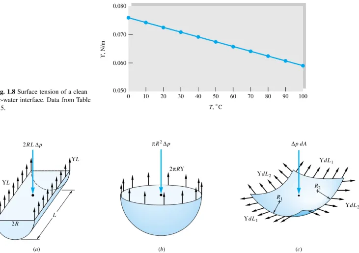
Actually, for all gases,cpand cvincrease gradually with temperature, and kdecreases gradually. Experimental values of the specific-heat ratio for eight common gases are shown in Fig. 1.3.

Many flow problems involve steam. Typical steam operating conditions are rela-tively close to the critical point, so that the perfect-gas approximation is inaccurate. The properties of steam are therefore available in tabular form [13], but the error of using the perfect-gas law is sometimes not great, as the following example shows.

EXAMPLE 1.6

Estimate and cpof steam at 100 lbf/in

2

and 400°F (a) by a perfect-gas approximation and (b) from the ASME steam tables [13].

Solution

First convert to BG units:p100 lbf/in214,400 lb/ft2,T400°F860°R. From Table A.4 the molecular weight of H2O is 2MHMO2(1.008)16.018.016. Then from Eq. (1.11)

the gas constant of steam is approximately

R 4 1 9 8 , . 7 0 0 1 0

6 2759 ft

2

/(s2°R) whence, from the perfect-gas law,

⬇ R p T 27 1 5 4 9 ,4 (8 0 6 0

0) 0.00607 slug/ft

3

Ans. (a)

From Fig. 1.3,kfor steam at 860°R is approximately 1.30. Then from Eq. (1.17),

cp⬇

k k R 1 1 1 .3 .3 0 0 (2 75 1 9)

12,000 ft2_/(s2_°R)

Ans. (a)

From Ref. 13, the specific volume vof steam at 100 lbf/in2_{and 400°F is 4.935 ft}3_{/lbm. Then}

the density is the inverse of this, converted to slugs:

1

v 0.00630 slug/ft

3

Ans. (b)

This is about 4 percent higher than our ideal-gas estimate in part (a). Reference 13 lists the value of cpof steam at 100 lbf/in

2

and 400°F as 0.535 Btu/(lbm°F). Convert this to BG units:

cp[0.535 Btu/(lbm°R)](778.2 ftlbf/Btu)(32.174 lbm/slug)

13,400 ftlbf/(slug°R)13,400 ft2_/(s2_°R)

Ans. (b)

1

Frank M White, 5 Ed.

Fluid Mechanics

Fourth Edition

Frank M. White

University of Rhode Island

About the Author

General Approach

Preface

Content Changes

Supplements

EES Software

Acknowledgments

Contents

1.1 Preliminary Remarks

Chapter 1

Introduction

1.2 The Concept of a Fluid

1.3 The Fluid as a Continuum

1.4 Dimensions and Units

冢

冣

冢

冣

冦

冧

冦

冧

1.5 Properties of the

Velocity Field

冕

冕

1.6 Thermodynamic Properties

of a Fluid

冢

冣

冢

冣